Front Propagation in Chaotic and Noisy Reaction-Diffusion Systems:
a Discrete-Time Map Approach

Abstract

We study the front propagation in Reaction-Diffusion systems whose reaction dynamics exhibits an unstable fixed point and chaotic or noisy behaviour. We have examined the influence of chaos and noise on the front propagation speed and on the wandering of the front around its average position. Assuming that the reaction term acts periodically in an impulsive way, the dynamical evolution of the system can be written as the convolution between a spatial propagator and a discrete-time map acting locally. This approach allows us to perform accurate numerical analysis. They reveal that in the pulled regime the front speed is basically determined by the shape of the map around the unstable fixed point, while its chaotic or noisy features play a marginal role. In contrast, in the pushed regime the presence of chaos or noise is more relevant. In particular the front speed decreases when the degree of chaoticity is increased, but it is not straightforward to derive a direct connection between the chaotic properties (e.g. the Lyapunov exponent) and the behaviour of the front. As for the fluctuations of the front position, we observe for the noisy maps that the associated mean square displacement grows in time as $t^{1/2}$ in the pushed case and as $t^{1/4}$ in the pulled one, in agreement with recent findings obtained for continuous models with multiplicative noise. Moreover we show that the same quantity saturates when a chaotic deterministic dynamics is considered for both pushed and pulled regimes.

I Introduction

In the last years the study of front dynamics has gained more and more relevance in many different fields, such as chemistry [1], biology [2], combustion [3]. In physics [4] the problem of front propagation is generally related to Reaction-Diffusion (RD) systems, and to the identification of the different dynamical regimes present in the model under study.

In this case the focus is often on the situation where RD fronts connect a stable state to an unstable one. Consider for instance the prototype equation for front propagation

$$\partial_{t}u=D\partial_{xx}u+f(u)\quad,$$ (1)

where $u=u(x,t)$ , $D$ is the diffusion coefficient and $f$ is a continuous function with two fixed points, $u=1$, stable, and $u=0$, unstable. This equation is usually referred to as Fisher-Kolmogorov-Petrovsky-Piskunov (FKPP) Equation [5, 6].

It is well known that if one considers an initial condition $u(x,0)$, different from zero in a bounded spatial region, a front develops connecting the two fixed points. The asymptotic leading edge, i.e. the semi-infinite region ahead of the front, has typically an exponential shape of the type $\exp(-\mu x+\lambda t)$. In principle, depending on the value of the spatial decay-rate $\mu$, the front speed can take a continuous set of values, namely $v(\mu)=\lambda/\mu$ [7].

However, for sufficiently localized initial conditions a unique speed $v_{\rm f}$ is selected, which is always bounded in the range $[v_{\rm lin},v_{\rm max}]$, with

$$v_{\rm lin}=\min_{\mu}v(\mu)=2\sqrt{Df^{\prime}(0)}$$ (2)

and

$$v_{\rm max}=2\sqrt{D\max_{0\leq u\leq 1}\,\frac{f(u)}{u}}\quad.$$ (3)

If the function $f(u)$ is concave, it is possible to prove that the propagation speed of the front coincides with the linear one, $v_{\rm f}\equiv v_{\rm lin}$ [9]. In literature this case is often referred to as pulled dynamics. The nonlinearities present in the system are not dynamically relevant, and a linearization about the unstable state is enough to fully describe the propagation of the front. As a result the front is indeed “pulled” by the spreading and growth of linear perturbations in the leading edge [8]. On the other hand, the function $f(u)$ being not concave is a necessary condition to have $v_{\rm f}>v_{\rm lin}$ [9]. This in turn corresponds to the pushed regime, where the nonlinearities are relevant to the dynamics and the front is “pushed” by its internal part [8].

Such a dynamical behaviour can also be studied when inhomogeneous environments are considered. A typical example is the photosensitive Belousov-Zhabotinsky chemical reaction. This system allows for an experimental realization of external noise, achieved via fluctuating illumination conditions [10]. The random environment can be mimicked by multiplicative noise terms in the corresponding RD equation – see for example [11, 12, 13, 14]. Under the effect of noise, the motion of the front can be decomposed into a global drift, characterized by a noise-renormalized speed, plus fluctuations, affecting the position of the front. Particularly the wandering of the front around its average position has been proven to be diffusive in the pushed case [12] and subdiffusive in the pulled one [14], with an associated mean square displacement growing in time respectively like $t^{1/2}$ and $t^{1/4}$.

Another natural way for erratic behaviors to occur in RD systems is via a chaotic underlying process. Even though so far only a limited number of papers has been devoted to the influence of chaotic dynamics on front propagation [17, 18], chaos is extremely relevant in RD systems describing chemical reactions [1], as well as in more general pattern forming systems [15]. Moreover, in the context of spatially extended chaotic systems many concepts have been borrowed from the study of front propagation into unstable steady states to describe the spreading of information [16].

In this paper we aim at taking up this issue again, by studying the front propagation in systems where an unstable fixed point is present and in addition the reaction dynamics is chaotic (or noisy). In the chaotic case the role of the stable fixed point in the usual FKPP problem is played by the chaotic phase. The most natural way of realizing this situation is to consider the case ${\bf u}\in R^{d}$ with $d\geq 3$ in the FKPP Equation, that is

$$\partial_{t}{\bf u}=D\partial_{xx}{\bf u}+{\bf f}({\bf u})\quad.$$ (4)

Here ${\bf u}=(u_{1},\dots,u_{d})$ and ${\bf f}=(f_{1},\dots,f_{d})$ is such that ${\bf u}=0$ is an unstable fixed point. Then, omitting diffusion, equation $d{\bf u}/dt={\bf f}({\bf u})$ can be chaotic and therefore we expect front solutions connecting the unstable state ${\bf u}=0$ to the chaotic state to be realizable.

However, as it is well known, there is an easiest way of introducing chaos in Eq. (1), without resting on the generalization to vectorial fields. Since our interest is in the qualitative effect of chaos in the reaction terms of (1), we can reduce ourselves to studying the simplest chaotic system, i.e. $1d$ discrete-time maps. As we shall see, $1d$ discrete-time maps allow for the analysis of both chaotic and non-chaotic dynamics, either in the pushed or in the pulled propagation regimes. Also, they can easily be generalized to include noise in the system, permitting thereby a comparison between deterministic and noisy dynamics.

Detailed numerical simulations of such systems show that in the pulled regime the front speed is basically determined by the unstable fixed point, while the chaotic (noisy) character of the reaction dynamics plays a limited role. In contrast, in the pushed regime the presence of chaos (noise) has some relevance, even if the relationship between chaotic properties and the front speed appears far from being trivial. The differences between the chaotic and the noisy situations are much more evident in the wandering of the front around its average position. The fluctuations of the front induced by the chaotic dynamics appear to be bounded on the examined time scale, while the presence of noise induces diffusive or sub-diffusive behaviour, in the pushed and pulled case respectively.

The discrete-time map approach is introduced in Section II, while the specific map models under study are introduced in Section III. The numerical results concerning front speed and front fluctuations are discussed in Section IV, and finally some concluding remarks are presented in Section V. The details on the integration algorithm and the estimation of the speed bounds for the discrete-time map approach are reported in Appendix A and B, respectively.

II Discrete-time map approach

With respect to Eq. (1), there exists a simple way for introducing discrete-time maps. This rests on considering the case when the reaction term acts in an impulsive way,

$$f(u)=\Delta tg(u)\sum_{n}\delta(t-n\Delta t)\quad,$$ (5)

where $g(u)$ is a function whose precise form is not relevant at this stage, and $\Delta t$ is the period of the forcing.

Consider now a kick given at time $t$. By direct integration of Eq. (1) between $t$ and $t+\varepsilon$, in the limit $\varepsilon\to 0$, we obtain

$$u(x,t+0^{+})=F(u(x,t))\quad,$$ (6)

where

$$F(w)=w+\Delta tg(w)\quad.$$ (7)

$F(v)$ is the reacting map. In other words we have written the evolution of the field between two successive kicks in terms of a simple map.

The remaining evolution of the field can be calculated noticing that from one kick to the next one, the evolution of the field is “free” because the impulsive reactive term by definition does not act. Indeed between $t+0^{+}$ and $t+\Delta t$, equation (4) reduces to the diffusion equation $\partial_{t}u=D\partial_{xx}u$, whose solution is known and allows for writing the complete evolution as:

$$u(x,t+\Delta t)$$ (8)

$$\qquad\quad=\frac{1}{\sqrt{4\pi D\Delta t}}\int_{-\infty}^{\infty}{\rm d}y\enskip{\rm e}^{-\frac{y^{2}}{4D\Delta t}}u(x-y,t+0^{+})$$ (9)

$$\qquad\quad=\frac{1}{\sqrt{4\pi D\Delta t}}\int_{-\infty}^{\infty}{\rm d}y\enskip{\rm e}^{-\frac{y^{2}}{4D\Delta t}}F[u(x-y,t)]\quad.$$ (10)

Let us notice that the above equation is nothing but the discrete-time version of the well known Feynman-Kac formula [19]. A similar approach has been recently introduced in [20] to study the two-dimensional dynamics of a front separating a chaotic state from a stable steady one.

We are only left with the evaluation of the convolution integral (10). Its numerical estimation can be performed employing a quite efficient and accurate algorithm recently introduced in [21]. A detailed description of the algorithm is given in Appendix A. Once the map is given, then its successive iterations account for the whole time evolution of the field according to Eq. (10). We remark that Eq. (10) is exact, i.e. it is not an approximation for small $\Delta t$ if Eq. (5) holds. For the sake of simplicity in the following we shall set $\Delta t=1$.

Of course the evolution of the field will be chaotic or not depending on the map. It is well known that the appropriate dynamical indicator to discriminate between chaotic and non-chaotic dynamics is the maximal Lyapunov exponent $\lambda$, which characterizes the divergence in time of nearby orbits. This exponent is estimated by applying a standard evaluation scheme [22] to the evolution of an infinitesimal perturbation $\delta u(x,t)$ of the reference orbit in the tangent space

$$\delta u(x,t+1)=\frac{1}{\sqrt{4\pi D}}\int_{-\infty}^{\infty}{\rm d}y\enskip{\rm e}^{-\frac{y^{2}}{4D}}$$ (11)

$$\qquad\qquad\qquad\qquad\times F^{\prime}[u(x-y,t)]\delta u(x-y,t)\quad.$$ (12)

The maximal Lyapunov exponent $\lambda$ is then defined as

$$\lambda=\lim_{t\to\infty}\frac{1}{t}\ln\frac{||\delta u(x,t)||}{||\delta u(x,0)||}\quad,$$ (13)

where $||\delta u(x,t)||^{2}=\int|\delta u(x,t)|^{2}dx$, $\lambda>0$ representing a signature of chaos.

III The Models

We describe first the two deterministic non-chaotic maps, which turn out to be useful to illustrate the general approach and to identify the different regimes present in the system. Starting from those models two generalization will be proposed, in order to assess whether the effects of noise or chaos on the system are relevant.

A Deterministic Non Chaotic Models

The first map we introduce has the purpose of reproducing the usual FKPP behaviour. As mentioned above, this is given by equation (1) where the function $f$ is chosen in such a way that $u=1$ is a stable fixed point and $u=0$ is an unstable one. Inspired by this feature, we propose a deterministic non-chaotic map with an unstable fixed point in $u=0$ (i.e. $F(0)=0$ and $|F^{\prime}(0)|>1$), and a stable one $u_{0}$, (i.e. $F(u_{0})=u_{0}$ with $|F^{\prime}(u_{0})|<1$). More specifically we define Map A as

$$F(u)=\left\{\begin{array}[]{cc}\alpha u,&\qquad 0\leq u<u_{1}\\ \beta u+c,&\qquad u_{1}\leq u<u_{2}\\ \gamma u+d,&\qquad u_{2}\leq u\leq 1\end{array}\right.$$ (17)

where $c=u_{1}(\alpha-\beta)$, $d=1-\gamma$ and $u_{2}=(d-c)/(\beta-\gamma)$ (see Fig. 1a).

The fixed point $u_{0}=1$ is stable provided that $|\gamma|$ is smaller than one. As we shall see, for this system the linear speed is $v_{\rm lin}=2\sqrt{D\ln\alpha}$ while the slope of the exponential part of the leading edge is $\mu_{\rm lin}=\sqrt{\ln\alpha/D}$. It is clear that we are always in the pulled situation if $\alpha\geq\beta$, while if $\beta$ is bigger than $\alpha$ pushed situations can be observed.

As a second reference model for non-chaotic dynamics we also introduce Map B. Now we set $u_{2}=1/2$ and $F(u_{2})=1$, while $c=1-\beta/2$, $u_{1}=c/(\alpha-\beta)$, $d=1-\gamma/2$ and $u_{0}=d/(1-\gamma)$. Also in this case we choose $|\gamma|<1$ in order to have a stable fixed point in $u_{0}$. This map is shown in Fig. 1b. The condition $\alpha<\beta$ allows again for pushed situations to be in principle observed.

FIG. 1.: Panel a): Map A. Since $\alpha>\beta$, the expected front propagation corresponds to the pulled case – see text. Panel b): Map B. In this case $\alpha<\beta$ makes it possible to observe pushed dynamics.

B Noisy Models

In order to mimic a random environment, in [12, 13, 14] the following noisy RD system was considered:

$$\partial_{t}u=D\partial_{xx}u+f(u)+g(u)\eta\quad,$$ (18)

with

$$f(u)=u(1-u)(a+u),\qquad g(u)=u(1-u)\quad.$$ (19)

The parameter $a$ is a control parameter, by tuning which it is possible to change the stability properties of the invaded state, thereby exploring both pushed and pulled dynamics [12]. The noise $\eta=\eta(x,t)$ is Gaussian, spatially and temporally $\delta$-correlated, and because of the chosen $g(u)$, it does not affect the fixed points $0$ and $1$. The multiplicative noise term present in (18) was first introduced phenomenologically as external noise in [12, 14], and then rederived in a broader context in [24]. Specifically, in [12, 14], due to the continuous nature of the model (18) it was proven that the appropriate prescription for the evaluation of the noise term was the Stratonovich one [23].

Relevant questions about such systems are typically related on one side to the computation of the renormalization due to noise of the propagation speed of the front, and on the other side to the identification of the general properties of the wandering of the front around its average position.

This scenario rests on the decomposition of the propagation of the front, solution of (18), into a global drift plus fluctuations. The global drift is associated to an average deterministic front, where the average is taken over the different realizations of the noise. This front obeys a deterministic field equation which can be obtained through a standard procedure from equation (18) (see for example [25]). In the simple case of the choice (19), this deterministic equation reduces to an equation with the same reaction term of (19) but with noise-renormalized parameters, implying thereby a renormalization of the front propagation speed [11]. Notice that this effect is related to the assumed Stratonovich prescription in the evaluation of the multiplicative noise term.

Of course the single realizations of the noise induce fluctuations in the shape of the front, which manifest themselves as fluctuations of the speed around its average value. This process induces in turn a wandering of the front around its average position. This can be characterized by the root mean square displacement of the front position $\Delta(t)$. As a result, the pulled and pushed regime differ noticeably. In particular, in the pushed regime the usual diffusive behavior is proven [12, 13] i.e. $\Delta(t)\sim t^{1/2}$ while in the pulled case a theoretical and numerical analysis shows that subdiffusion occurs, with $\Delta(t)\sim t^{1/4}$ [14].

Having in mind all this, and starting from the deterministic non-chaotic models introduced in the previous subsection, namely Map A and Map B, we introduce the corresponding noisy maps. Even if a direct comparison between the continuous model and our discrete-time maps is beyond the scope of the present paper, nevertheless we aim at assessing if the main features of the continuous FKPP equation with multiplicative noise are still observable for periodically forced discrete systems.

As a first choice, we consider the stochastic version of Map A reported in Eq. (17). We shall refer to this model as Map NA and we expect that it will be qualitatively equivalent to the noisy FKPP Equation, Eq. (19). Of course the insertion of noise can be performed on any of the three segments of the map, identified by their slopes $\alpha$, $\beta$, $\gamma$. Our strategy will be of inserting noise on one of them, by keeping fixed the other ones. For instance we can consider a situation where both $\beta$ and $\gamma$ are fixed while $\alpha$ is chosen randomly at any space-time point as

$$\alpha(x,t)=\alpha_{0}+\eta(x,t)\quad.$$ (20)

Here the noise $\eta$ is distributed according to a flat distribution defined in the interval $[-A,A]$, and is $\delta$-correlated both in space and time. The model is constructed in such a way to maintain $u=0$ and $u=1$ as fixed points.

The second type of noisy map that we analyze can be introduced starting from Map B. In this case the noise is added to the parameter $\gamma$ and it has again the same flat bounded distribution of Map NA and the same correlator. In this case, the restriction that $|\gamma_{0}\pm A|$ be smaller then one forces the map to have a unique unstable fixed point $u=0$ but an infinite number of different stable fixed points $u=u_{0}(\gamma)$. As a matter of fact the interior region of the front, developing from the state $u=0$, oscillates stochastically around the average fixed point $\langle u_{0}\rangle=d/(1-\gamma_{0})$. We shall refer to this model as Map NB. It will be a benchmark to understand what the effects are of the noise, when it affects the saturated part of the front.

C Chaotic Models

Modifying Map B it is possible to introduce a chaotic version of the FKPP Equation, which we shall term Map CB. This map is defined by keeping it identical to Map B for $u\leq u_{2}=1/2$ and modifying the part in the interval $1/2<u\leq 1$ in the following way:

$$F(u)=\left\{\begin{array}[]{cc}\gamma u+d,&\qquad u_{2}\leq u\leq u_{3}\\ \delta u+e,&\qquad u_{3}\leq u\leq 1\end{array}\right.$$ (23)

where $\gamma=1/(1/2-u_{3})<0$, $\delta=1/(1-u_{3})>0$, $d=1-\gamma/2$ and $e=1-\delta$, while $u_{3}$ is arbitrarily chosen with the restriction to belong to the interval $1/2<u_{3}\leq 1$. Map CB is represented in Fig. 2.

FIG. 2.: Map CB. A variation of the value of $u_{3}$ induces a modification of the corresponding Lyapunov exponent.

Notice that the fixed points of the map ($u=0$ and $u_{0}$) are both unstable, because now the value of $|\alpha|$ and $|\gamma|$ are bigger than one. With these conditions, the map appears to be always chaotic, i.e. the maximal Lyapunov exponent $\lambda$ is positive.

As shown in the next section, in this case a localized initial disturbance of the unstable state $u=0$ will grow and spread along the system. As a consequence, a front will develop connecting the unstable fixed point $u=0$ to a chaotic phase, playing the role of the invading state.

IV Numerical Results and Discussion

Let us first present some qualitative results concerning the main features of deterministic non-chaotic fronts (Map B), noisy fronts (Map NB), and chaotic fronts (Map CB), in both the pushed and pulled regimes.

In all the examined cases, the chain length was $L=30,000$, and it was initially set everywhere to $0$, with exception of a few sites in the center of the chain, which were initialized with a disturbance amplitude of ${\cal O}(1)$.

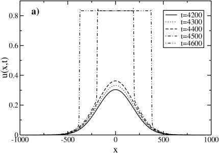
FIG. 3.: Front evolution for the FKPP equation with Map B in a) the pushed regime and b) the pulled one. In the pushed regime the values of the parameters are $\alpha=1.001$ and $\beta=5.0$, while in the pulled one we set $\alpha=1.8$ and $\beta=2.5$. In both cases $D=4$ and $\gamma=-1/2$.

In Fig. 3a and 3b we show the deterministic non-chaotic behaviour of pushed and pulled fronts respectively. The corresponding dynamics is selected by changing the relative weight of the parameters $\alpha$ and $\beta$, as explained in Section III A. The realization of the pushed or pulled regime is checked by direct measurement of the front speed (see the precise definition in the next Section). The linear speed corresponding to case shown in Fig. 3a is $v_{\rm lin}=0.126$, while the measured value is $v_{\rm f}=1.444$, confirming thereby the realization of the pushed regime. As for Fig. 3b, we measure $v_{\rm f}=v_{\rm lin}$, with $v_{\rm lin}=3.066$, corresponding indeed to pulled dynamics.

In the pushed case it is evident an abrupt jump from an initial evolution where the dynamics is ruled by the linear mechanisms (characterized by a Gaussian shaped perturbation propagating with velocity $v_{\rm lin}$) to a situation where nonlinearities set in and the front saturates in its central part and starts propagating with a velocity $v_{\rm f}>v_{\rm lin}$. In contrast, in the pulled situation (depicted in Fig. 3b) the transition from the initial Gaussian perturbation to a saturated propagating front is smoother, since now the only mechanism responsible for propagation is the linear one and the speed does not increase above the linear value.

Noisy front propagations as given by Map NB are shown in Fig. 4a and 4b for pushed and pulled dynamics respectively. In this case the values of the parameters are the same as in Fig. 3, with the only exception of the $\gamma$ parameter, which is the one affected by the noise.

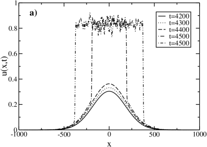
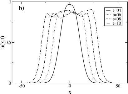
FIG. 4.: Front evolution for the FKPP equation with Map NB in a) the pushed regime and b) the pulled one. In the pushed regime the values of the parameters are $D=4$, $\alpha=1.001$ and $\beta=5.0$, while in the pulled one we set $D=4$, $\alpha=1.8$ and $\beta=2.5$. The noise is set on the parameter $\gamma$ with $A=0.45$, with $\gamma_{0}=-1/2$.

It is remarkable the fact that there seems to be no effect of noise on the value of the speed. As a matter of fact, the measured speeds have the values $v_{\rm f}=1.444$ (against the linear value $v_{\rm lin}=0.126$) in the pushed case and again $v_{\rm f}=v_{\rm lin}=3.066$ in the pulled one. These values coincide with the ones obtained in the deterministic non-chaotic dynamics. However, by analogy with the continuous model, we could naively expect a renormalization of the front speed to occur in both pulled and pushed regimes. The fact that this does not seem to be the case is related to the intrinsic discreteness of our models. In the next Section we shall analyze this point in greater detail.

Our results for the chaotic models are shown in Fig. 5, again for both pushed and pulled dynamics.

FIG. 5.: Front evolution for the FKPP equation with Map CB with $u_{3}=1$ in a) the pushed regime and b) the pulled one. The parameters $\alpha$, $\beta$,and $D$ are again chosen as in the previous figures, while the parameter $\gamma$ is now set to the value $\gamma=-2$. The snapshot shown in Panel b is taken at time $t=90$.

As it is evident by comparison of Fig. 4 and 5, chaos and noise seem to affect in a qualitatively equivalent way the front structure, at least when the noise is set on the $\gamma$ parameter. This could suggest the possibility of easily building up an effective noisy model for a general underlying chaotic dynamics. However as we shall see in the next Section, an effective equivalence between the two models is far from being trivial, due to the different role played by noise and chaos on the renormalization properties of the speed of the front. This is clear in the pushed regime, where the front speed takes the value $v_{\rm f}=1.276$, smaller than in the corresponding non-chaotic and noisy models, indicating a deep difference between the respective dynamics.

Finally notice that all the fronts shown in the previous figures manifest the same dynamical evolution at short times up to $t^{*}={\cal O}(1/\ln(\alpha))$. As a matter of fact, in the pushed case the front evolution associated to the three maps become distinguishable at times of the order of $t=4,400$, with $\alpha=1.001$, while for the fronts in the pulled regime the evolution of the three maps are practically identical up to time $t=12$, since now the $\alpha$ parameter is much bigger (namely, $1.8$). Afterwards it becomes possible to distinguish the different evolutions in both situations.

In order to investigate at a more quantitative level the different dynamical behaviour of fronts in presence of noisy or chaotic dynamics, we analyze now the front propagation speed and the fluctuations of the front position.

A Speed of the Front

It is not difficult to show that for the discrete-time map version of the FKPP Equation, the propagation speed $v_{\rm f}$ is always bounded in the interval $[v_{\rm lin},v_{\rm max}]$, where

$$v_{\rm lin}=2\sqrt{D\ln(F^{\prime}(0))}$$ (24)

and

$$v_{\rm max}=2\sqrt{D\ln\left[\max_{0\leq u\leq 1}\,\frac{F(u)}{u}\right]}\quad.$$ (25)

Justification of (24) and (25) is given in Appendix B. As mentioned before, if $v_{\rm f}=v_{\rm lin}$, then the dynamics is pulled, while if $v_{\rm f}>v_{\rm lin}$ the corresponding dynamics will be pushed.

From the numerical point of view, the measurement of the speed has been performed in the following way. After having initialized to zero all the chain apart a localized disturbance $u(x,0)={\cal O}(1)$ for $-\xi\leq x\leq\xi$, at each time step the rightmost $r(t)$ and the leftmost position $l(t)$ of the front are considered,

$$r(t)=\max\{x\;|\;u(x,t)>\vartheta\}\quad,$$ (26)

$$l(t)=\min\{x\;|\;u(x,t)>\vartheta\}\quad,$$ (27)

where $\vartheta$ is a preassigned threshold. The position of the front is simply $x_{f}^{r}(t)=r(t)-\xi$ or $x_{f}^{l}(t)=\xi-l(t)$, depending on which of the two moving fronts is considered, and the speed results in

$$v_{\rm f}=\lim_{t\to\infty}\frac{x_{f}^{r}(t)-x_{f}^{l}(t)}{2t}\quad.$$ (28)

We have verified that $v_{\rm f}$ does not depend on the chosen threshold and obviously the time limit reported in (28) should be taken after the limit $L\to\infty$.

We present now a more detailed investigation of the dependence of the speed on both noise and chaos. Consider first Fig. 6. Our main result is that the “structural” features of the map (its concave or convex character) are sufficient to provide information about the type of front propagation observable and the chaotic, noisy or non-chaotic nature of the dynamics seems to be secondary. This conclusion relies on the measurement of the front speed for Map B, Map NB, and Map CB with $u_{3}=1$. We have performed the simulation by keeping $\beta=2.5$ and $\gamma=-1/2$ fixed, and changing the $\alpha$ values in the interval $1\leq\alpha\leq 2$. As shown in Fig. 6 $v_{\rm f}>v_{\rm lin}$ for $\alpha<1.4$, and therefore for $\alpha>1.4$ the linear mechanism prevails on the nonlinear one and the front is pulled from the linear instability of the leading edge. The same choice of parameters has been done also for maps CB ($u_{3}=1$) and NB in such a way that the three maps essentially coincide for $u<u_{2}=1/2$.

FIG. 6.: Front speeds $v_{\rm f}$ as a function of the parameter $\alpha$ for the Map CB ($u_{3}=1$) (triangles), B (circles) and NB (diamonds) with $\beta=2.5$ and $D=4$. The dashed line indicates $v_{\rm max}=2\sqrt{D\ln 2}$ and the solid one $v_{\rm lin}=2\sqrt{D\ln\alpha}$. The length of the chain is $L=10,000$, the front has been followed for a time $t=1,600$, and the average is performed over $400$ different initial conditions.

As we can observe from Fig. 6 the speeds of the fronts are almost identical in the three cases. Only in the strongly pushed regime, that is for values of $\alpha$ very close to 1, the propagation for the chaotic model appears to be slightly slower than in the other models, but the discrepancy is indeed very small. For values of $\alpha$ as small as $\alpha=1.001$ the observed values for the velocities obtained for both Map B and NB are $v_{\rm f}=1.965$, while for Map CB (with $u_{3}=1$) we obtain $v_{\rm f}=1.884$, corresponding to a discrepancy of the order of 4%.

In order to better analyze these findings, we investigate the dependence of the speed separately as a function of the intensity of the noise $A$ and of the Lyapunov coefficient $\lambda$.

As far as the effect of noise is concerned, we consider first Map NB. We set noise on the three parameters of the map, i.e. $\alpha$, $\beta$ and $\gamma$, but the corresponding changes of the speed appear basically negligible in all cases.

More interesting is the case corresponding to Map NA. In this situation, there is still no effect of noise in the pulled regime, while in the pushed case we find a decrease of the speed with the noise amplitude, for noise added to any of the three parameters. Anyway, the strongest decrease has been observed when the noise affects the parameter $\gamma$. This case is the one reported in Fig. 7. At this point it is worth to remark that the very weak velocity renormalization due to noise observed in the present context is not in contradiction with the results reported in [11], where a noticeable variation of the front speed with the noise amplitude was found.

This is so because the intrinsic discrete nature of our system does not leave room to any ambiguity in the definition of the multiplicative noise term (the so-called Ito-Stratonovich dilemma [23]). As a matter of fact, in the limit $\Delta t\to 0$ our model would correspond to a continuous model with multiplicative noise inserted according to the Ito’s prescription.

FIG. 7.: Dependence of the front speed $v_{\rm f}$ on the intensity of noise $A$ in Map NB. Here the noise is inserted on the parameter $\gamma$, with $\gamma_{0}=-1/2$. The values of the other parameters are $\alpha=1.001$ and $\beta=5$ (strongly pushed), and $D=4$.

The second point worth of investigation is the effect of chaos. In this case we performed a measurement of the speed of the front as a function of the Lyapunov coefficient in the strongly pushed regime. A different degree of chaoticity is obtained by tuning the value of $u_{3}$ in Map CB, and can be evaluated via the corresponding Lyapunov exponent $\lambda$. Our results are plotted in Fig. 8.

The speed exhibits a strong decrease as a function of $\lambda$, which seems to indicate a behaviour similar to noisy case. However, by direct comparison of Figs. 7 and 8, it appears evident that chaos affects the system in a quite more relevant way then noise.

FIG. 8.: Front speeds $v_{\rm f}$ as a function of $\lambda$ for the Map CB. The values of the parameters are in this case $D=4$, $\alpha=1.001$, $\beta=5$, $u_{1}=0.3751$. The length of the chain is fixed for all the simulations to $L=30,000$, the front has been followed for a time $t=5,000$, and the average are performed typically over $1,000$ different initial conditions.

B Fluctuations of the front

Now we consider the root mean square displacement of the front position $x_{f}(t)$,

$$\Delta(t)=\sqrt{\langle x_{f}^{2}(t)\rangle-\langle x_{f}(t)\rangle^{2}}\quad,$$ (29)

where the average is taken over different initial conditions for the chaotic case and over many distinct noise realizations for the noisy case. Different scalings for $\Delta(t)$ are observed depending on the type of map and on how the noise enters the dynamics.

Let us examine first Map NA. We have studied the three different cases corresponding on applying noise on $\alpha$, $\beta$ or $\gamma$. In the pulled case the noise does not induce any wandering of the front when it is added to $\beta$ or $\gamma$: In such cases $\Delta(t)\to const.$ in the limit $t\to\infty$. In contrast, if the noise is applied to the $\alpha$ parameter, sub-diffusive behavior is indeed observed. These results can be justified recalling that in the pulled case the dynamics of the front is determined in the leading edge. This region corresponds to small $u$ values, and therefore only a (stochastic) change in $\alpha$ is expected to affect the behavior of the system.

FIG. 9.: Fluctuations $\Delta(t)$ as a function of time in a log-log scale for Map NA, with noise on the $\alpha$-parameter. Namely $\alpha_{0}=10$, $A=4$, $\beta=1.0$, $\gamma=-0.2$, and $D=4$. The data have been averaged over $4,400$ different noise realizations for a chain of length $L=60,000$, with bounded noise. The dashed line refers to a power law $t^{q}$ with exponent $q=1/4$. In this case the linear speed is $v_{\rm lin}=6.0697$, while the measured one is $v_{\rm f}\simeq 6.069$: we are clearly in the pulled case.

On the other hand, in the pushed regime we observe that in all three cases the noise has the same effect on the front wandering and it leads to a diffusive behaviour for the front positions (see Fig. 10). This effect is also reasonable since now the front propagation is also related to the regions where the field takes values of ${\cal O}(1)$, and not only to the leading edge. Therefore the effect of the noise will be equally relevant, independently of what parameter it is applied to.

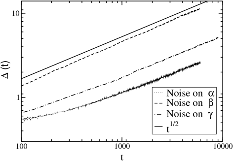
FIG. 10.: Fluctuations $\Delta(t)$ as a function of $t$ in a log-log scale for Map NA, with noise added to the parameter $\alpha$ (with values of the parameters $\alpha_{0}=2$, $A=1$, $\beta=6$, and $\gamma=-0.2$), $\beta$ (with values of the parameters $\alpha=2$, $\beta_{0}=6$, $A=3$ and $\gamma=-0.2$) or $\gamma$ (with values of the parameters $\alpha=1.1$, $\beta=2.5$, $\gamma_{0}=-0.5$, and $A=0.4$); always $D=4$. The solid line represents the power law $t^{q}$ with $q=1/2$. We are in the pushed situation since $v_{\rm f}>v_{\rm lin}$ for all three examined cases. Namely for noise acting on $\alpha$, $v_{\rm f}=4.436$ and $v_{\rm lin}=3.330$; for noise acting on $\beta$ the linear speed is the same while $v_{\rm f}=4.406$; for noise acting on $\gamma$, $v_{\rm lin}=1.235$, while $v_{\rm f}=3.075$.

To complete the analysis related to the noisy dynamics we have also considered Map NB with noise on the parameter $\gamma$ only. In the pulled case, similarly to the Map NA case, we observe saturation of the root mean square displacement $\Delta(t)$. In the pushed case $\Delta(t)$ indeed grows in time, but within our time window and for the examined parameters ($\alpha=1.9$, $\beta=2.5$, $\gamma_{0}=-0.5$ and $A=0.4$, with $v_{\rm f}=v_{\rm lin}=3.2046$), we do not observe any clear scaling.

Finally we address the chaotic case. Our results are reported in Fig. 11.

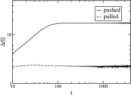
FIG. 11.: Root mean square displacement $\Delta(t)$ as a function of time for Map CB with $u_{3}=1$. The values of the parameters are in this case $\alpha=1.1$ (pushed) and $\alpha=1.8$ (pulled), $\gamma=2.5$, $\beta=-2$, and $D=4$. The length of the chain was $L=60,000$ and the average was performed over 2,000 initial conditions.

In this situation, in contrast with the stochastic case, we observe for the pulled as well as for the pushed regime that $\Delta(t)$ saturates to a constant values. We have verified this for Map CB with $u_{3}=1$ (see Fig. 11). An analogous result has been observed by Rudzick et al. [17] for a Coupled Map Lattice (CML) model. In that case a diffusive behaviour for the wandering of the front position is observed for small diffusive coupling, while for sufficiently strong coupling $\Delta(t)$ is shown to saturate. The authors of [17] argue that this result can be explained as follows. For small couplings, the spatial correlation between adjacent sites is negligible on a distance corresponding to their lattice spacing. Therefore, the successive positions occupied by the front in its time evolution will be completely decorrelated, and the front dynamics induced by the local chaotic evolution can be described in term of a stochastic process. In contrast, when the coupling becomes large enough, the lattice sites become correlated on a length scale larger than the lattice spacing, and this implies that a description of the front evolution in terms of a stochastic process in not appropriate any longer, not even for chaotic maps. Notice that the CML model is a spatially discrete model, which can be considered a fair approximation of a continuous space system only for sufficiently large diffusive couplings. Therefore in our case we always expect that for chaotic maps $\Delta(t)$ cannot grow indefinitely in time, and saturation is the only behavior observable. This indicates that the chaotic evolution cannot be simply reduced to some erratic behaviour sharing common dynamical features with the noisy systems.

V Concluding Remarks

In this paper we have studied the front propagation in reaction diffusion systems with a periodically forced reaction term. For this case we have been able to rewrite the evolution of the system as a convolution of a spatial propagator and a discrete-time map. By implementing a quite efficient algorithm for the evaluation of the convolution integral, we have numerically studied the front dynamics for deterministic non-chaotic and chaotic maps as well as for noisy maps. An analogy with the usual FKPP problem can be drawn for non-chaotic maps, allowing to obtain the expression for the lower and upper bound for the speed of the front. Moreover, even when the reaction dynamics presents an unstable fixed point coexisting with a chaotic (or noisy) behaviour, the analogy with the FKPP problem still holds, once the chaotic (noisy) phase is identified with the stable fixed point of the usual FKPP reaction term. In the pulled regime the presence of chaos (noise) plays a poor role and the front speed $v_{\rm f}$ is essentially determined by the dynamical evolution around the unstable fixed point. On the contrary in the pushed case $v_{\rm f}$ depends in a nontrivial way on the details of the chaotic (noisy) behaviour. Unfortunately, the relationship between the chaotic properties (e.g. the Lyapunov exponent) and the values of the observed $v_{\rm f}$ does not appear simple. In particular, the effect of chaos seems to be much stronger than that related to the noise: e.g. $v_{\rm f}$ changes noticeably for chaotic reaction dynamics at varying the Lyapunov exponent, while it remains almost constant as a function of the strength of the noise. In contrast, the noise induces a wandering of the front around its average position, which is diffusive in the pushed case and sub-diffusive in the pulled one. Our results confirm the same scaling laws found in continuous models with multiplicative noise [12, 13, 14] for the time evolution of the mean square displacement $\Delta(t)$ associated to the front position fluctuations, namely $\Delta(t)\sim t^{1/2}$ in the pushed case and $\Delta(t)\sim t^{1/4}$ in the pulled situation. This suggests that such results are universal in that they do not depend on the details of the system. When a chaotic dynamics is considered both in the pushed and in the pulled case a saturation of $\Delta(t)$ to a constant value is observed, and this is consistent with previous results obtained for coupled map lattice with strong diffusive couplings [17].

A Details on the integration algorithm

Let us now present the numerical details concerning the integration of Eq. (10),

$$u(x,t+\Delta t)=$$ (A1)

$$\qquad\frac{1}{\sqrt{4\pi D\Delta t}}\int_{-\infty}^{\infty}{\rm d}y\enskip{\rm e}^{-\frac{y^{2}}{4D\Delta t}}F[u(x-y,t)]\quad,$$ (A2)

which represents the convolution between the field at time $t+\varepsilon$ (i.e. $u(x,t+\varepsilon)=F[u(x,t)]$) and the Gaussian Kernel

$$K(x)=\frac{1}{\sqrt{4\pi D\Delta t}}\enskip{\rm e}^{-\frac{x^{2}}{4D\Delta t}}\quad.$$ (A3)

The integration (A2) can be performed on a computer once the field is discretized on a grid of resolution $\Delta x$. The integral reported in Eq. (A2) reduces then to the sum

$$u(i\Delta x,t+\Delta t)=$$ (A4)

$$\qquad\qquad\sum_{m=-N/2}^{N/2}K(m\Delta x)F[u((i-m)\Delta x,t)]\quad,$$ (A5)

where the system length is $L=N\Delta x$ and periodic boundary conditions are assumed along the chain.

In order to improve the integration speed we have restricted the sum (A5) to a small number $M$ of neighbours of the site $i$ and to ensure a good precision the true kernel has been substituted by a “modified” kernel $C(m)$, chosen to minimize the integration error. With these choices Eq. (A5) now reads:

$$u(i\Delta x,t+\Delta t)=$$ (A6)

$$\qquad\qquad\sum_{m=-M}^{M}C(m)u((i-m)\Delta x,t+\varepsilon)\quad.$$ (A7)

The problem is now to determine the coefficients $\{C(m)\}$ for $m=-M,\dots,M$. In order to do this, we first suppose that an appropriate Fourier basis made up of $(2M+1)$ elements, able to well approximate the field on the chosen grid, can be written as

$$\left\{\exp[j(k\alpha)x]\right\}\quad,$$

where the parameter $\alpha$ will be determined later. By rewriting Eq. (A7) on this basis one is left with the following set of equations:

$$\sum_{m=-M}^{M}C(m)\exp[-j(k\alpha)m\Delta x]$$ (A8)

$$\qquad\qquad\qquad\qquad=\exp[-(k\alpha)^{2}D\Delta t]\quad.$$ (A9)

Due to the Kernel symmetry we can reduce the system of $(2M+1)$ equations (A9) to a set of $M$ equations. This because the elements of the Kernel are symmetric around $m=0$ (i.e. $C(m)=C(-m)$), and are related by the normalization condition

$$C(0)=1-\sum_{m\neq 0}C(m)\quad.$$

We can determine the $M$ independent elements of the Kernel $C(m)$ by solving the system (A9) as a function of the parameter $\alpha$, once the integration time step $\Delta t$, the diffusion coefficient $D$, and the spatial resolution $\Delta x$ are fixed. The optimal choice of the parameter $\alpha$ is achieved by requiring that the first six cumulants of the discretized Kernel reproduce those of the true Kernel within a precision of one part over a million and that the quadratic sum $\sum_{m=-M}^{M}C^{2}(m)$ is minimal. In the present paper, we have always used $D=4$, $\Delta t=\Delta x=1$ with $M=15$ and a parameter value $\alpha=0.13$.

This integration scheme has been previously introduced as a possible alternative to the usual pseudo-spectral codes to evaluate the dynamical evolution of the complex Ginzburg-Landau equation and of the Fitzhugh-Nagumo equation in one and two dimensions [21].

B The speed bounds for discrete time maps

The linear speed (24) for discrete maps can be obtained with simple consideration just following the standard reasoning used for the derivation of $v_{\rm lin}$ in the continuous time limit:

$$\frac{\partial}{\partial t}u=D\nabla^{2}u+f(u)\quad.$$ (B1)

As we have already mentioned, the leading edge of the propagating front has an exponential shape:

$$u(x,t)\simeq e^{-\mu x+\lambda(\mu)t}\quad.$$ (B2)

Inserting (B2) in (B1) and linearizing around $u=0$ one obtains:

$$\lambda(\mu)=D\mu^{2}+f^{\prime}(0)\quad.$$ (B3)

A stationary phase argument gives a selection criterion which allows for the determination of the front speed as

$$v_{\rm lin}=\min_{\mu}\frac{\lambda(\mu)}{\mu}=2\sqrt{{D}f^{\prime}(0)}\quad.$$ (B4)

Let us consider now the discrete-time reaction case,

$$\frac{\partial}{\partial t}u=D\nabla^{2}u+\sum_{n=-\infty}^{\infty}g(u)\delta(t-n)\quad,$$ (B5)

where we have adopted $\Delta t=1$. Indicating with $F(u)$ the reacting map one gets:

$$u(x,t+0^{+})=F(u(x,t))\quad,$$

and integrating the diffusion equation $\partial_{t}u=D\nabla^{2}u$ between $t+0^{+}$ and $t+1$ one obtains:

$$u(x,t+1)=\frac{1}{\sqrt{4\pi D}}\int e^{-\frac{w^{2}}{4D}}F\left(u(x-w,t)\right){\mathrm{d}}w\quad,$$ (B6)

Assuming the shape (B2) and linearizing around $u=0$, i.e.: $F(u)\simeq F^{\prime}(0)u$, a simple Gaussian integration gives:

$$e^{\lambda(\mu)(t+1)-\mu x}\simeq e^{\ln F^{\prime}(0)+D\mu^{2}-\mu x+\lambda(\mu)t}\quad.$$

The above result implies

$$\lambda(\mu)=\ln F^{\prime}(0)+D\mu^{2}\quad,$$

which is nothing but Eq. (B3) now with $\ln F^{\prime}(0)$ in place of $f^{\prime}(0)$. The same selection criterion gives

$$v_{\rm lin}=2\sqrt{D\ln F^{\prime}(0)}\quad.$$ (B7)

In order to estimate $v_{\rm max}$ in the discrete case, let us consider again the continuous equation (B1) with the shape of $u(x,t)$ given by (B2). It is straightforward to show that

$$\lambda(\mu)\leq D\mu^{2}+\max_{0\leq u\leq 1}\frac{f(u)}{u}\quad.$$ (B8)

From the above inequality it can be shown that

$$v_{\rm max}=2\sqrt{D\max_{0\leq u\leq 1}\,\frac{f(u)}{u}}\quad.$$ (B9)

In the discrete case we write the following inequality

$$u(x,t+1)\leq\frac{1}{\sqrt{4\pi D}}\left(\max_{0\leq u\leq 1}\frac{F(u)}{u}\right)$$ (B10)

$$\qquad\qquad\qquad\qquad\times\int e^{-\frac{w^{2}}{4D}}u(x-w,t){\mathrm{d}}w\quad,$$ (B11)

and assuming that the leading edge has the shape reported in (B2) one obtains

$$\lambda(\mu)\leq D\mu^{2}+\ln\left[\max_{0\leq u\leq 1}\frac{F(u)}{u}\right]\quad.$$ (B12)

This equation is analogous to (B8) therefore in the discrete case the upper bound for the speed is now

$$v_{\rm max}=2\sqrt{D\ln\left[\max_{0\leq u\leq 1}\,\frac{F(u)}{u}\right]}\quad.$$ (B13)

REFERENCES

- [1] R. Kapral and K. Showalter (Ed.s), Chemical waves and patterns, Kluwer Academic Publishers, 1995.
- [2] J.D. Murray, Mathematical Biology, 2nd ed., Springer-Verlag, Berlin, 1989.
- [3] N. Peters, Turbulent Combustion, Cambridge University Press, Cambridge, 2000.
- [4] J. Xin, SIAM Review 42, 161 (2000).
- [5] R.A. Fisher, Ann. Eugenics 7, 355 (1937).
- [6] A. Kolmogorov, I. Petrovsky, and N. Piskunov, Bull. Univ. Moskou Ser. Int. Se. A 1(6), 1 (1937).
- [7] W. van Saarloos, Phys. Rev. A37, 211 (1988); Phys. Rev. A39, 6367 (1989).
- [8] U. Ebert and W. van Saarloos, Physica D 146, 1 (2000).
- [9] D.G. Aranson and H.F. Weinberger, Adv. Math. 30, 33 (1978).
- [10] I. Sendiña-Nadal, S. Alonso, V. Pérez-Muñuzuri, M. Gómez-Gesteira, V. Pérez-Villar, L. Ramírez-Piscina, J. Casademunt, J.M. Sancho and F. Sagués, Phys. Rev. Lett. 84, 2734 (2000).
- [11] J. Armero, J.M. Sancho, J. Casademunt, A.M. Lacasta, L. Ramírez-Piscina, and F. Sagues, Phys. Rev. Lett.76, 3045 (1996).
- [12] J. Armero, J. Casademunt, L. Ramírez-Piscina, and J.M. Sancho, Phys. Rev. E58, 5494 (1998).
- [13] A. Rocco, J. Casademunt, U. Ebert, and W. van Saarloos, cond-mat/0106081.
- [14] A. Rocco, U. Ebert, and W. van Saarloos, Phys. Rev. E62, R13 (2000).
- [15] M.C. Cross and P.C. Hohenberg, Rev. Mod. Phys. 65, 851 (1992).
- [16] A. Torcini, P. Grassberger, and A. Politi, J. Phys. A 27, 4533 (1995); A. Torcini and S. Lepri, Phys. Rev. E55, R3805 (1997); M. Cencini and A. Torcini Phys. Rev. E63, 056201 (2001).
- [17] O. Rudzick, A. Pikovsky, C. Scheffczyk, and J. Kurths, Physica D 103, 330 (1997).
- [18] C. Storm, W. Spruijt, U. Ebert and W. van Saarloos, Phys. Rev. E61, R6063 (2000).
- [19] M. Freidlin, Markov processes and differential equations: asymptotic problems, Birkhäuser, Boston, 1996.
- [20] J.W. Kim, J. Y. Vaishnav, E. Ott, S.C. Venkataramani, and W. Losert, Phys. Rev. E64, 016215 (2001).
- [21] A. Torcini, H. Frauenkron, and P. Grassberger, Phys. Rev. E55, 5073 (1997); M. Nitti, A. Torcini, and S. Ruffo, Int. J. Mod. Phys. C 10, 1039 (1999).
- [22] I. Shimada, and T. Nagashima, Prog. Theor. Phys. 61, 1605 (1979); G. Benettin, L. Galgani, A. Giorgilli, and J.M. Strelcyn, Meccanica 9, 21 (1980).
- [23] C.W. Gardiner, Handbook of Stochastic Methods for Physics, Chemistry and the Natural Science, Springer-Verlag, Berlin, 1983.
- [24] G. Tripathy, A. Rocco, J. Casademunt, W. van Saarloos, Phys. Rev. Lett. 86, 5215 (2001).
- [25] A. Rocco, J. Casademunt, L. Ramírez-Piscina, in preparation.