Equilibrium Distribution of the Inherent States and
their Dynamics in Glassy Systems and Granular Media

Abstract

The present paper proposes a Statistical Mechanics approach to the inherent states of glassy systems and granular materials, following the original ideas developed by Edwards for granular materials. Two lattice models, a diluted Spin Glass and a system of hard-spheres under gravity, introduced in the context of glassy systems and granular materials, are evolved using a “tap dynamics” analogous to that of experiments on granular materials. The asymptotic macrostates, reached by the system, are shown to be described by a single thermodynamical parameter, and this parameter to coincide with the temperature, called the “configurational temperature”, predicted assuming that the distribution among the inherent states satisfies the principle of maximum entropy.

The thermodynamics of macroscopic systems evolving at equilibrium is well described by Statistical Mechanics. However there are many systems, typically found in “frozen states”, where they do not evolve at all. These are, for example, supercooled liquids quenched at zero temperature in states, called inherent states [1, 2], corresponding to the local minima of the potential energy in the 3N-dimensional configuration space of particle coordinates. Granular materials [3] at rest are another important example of system frozen in mechanically stable microstates. Grains are “frozen” because, due to their large masses [3], the thermal kinetic energy is negligible compared to the gravitational energy; thus the external bath temperature, $T_{bath}$, can be considered equal to zero (by analogy with supercooled liquids, we call these mechanically stable configurations inherent states).

In this paper, following the original ideas by Edwards for granular materials [4] we attempt to develop a unified Statistical Mechanics approach for the inherent states of glassy systems and granular materials along the line of Ref. [5]. The connection between Edwards approach and recent developments on glass theory has received much attention [6, 7, 8, 9, 10, 11, 12].

The first step is to introduce a suitable dynamics which allows to explore the configurations of the inherent states. In granular materials the dynamics, from one stable microstate to another, can be induced by sequences of “taps”, in which the energy is pumped into the system in pulses. Due to inelastic collisions the kinetic energy is totally dissipated after each tap, and the system is again frozen in one of its inherent states [13]. Similarly, in glass formers at zero temperature the dynamics, from one inherent state to another, can be induced by sequences of taps, where each tap consists in raising the bath temperature and, after a lapse of time $\tau_{0}$, quenching it back to zero. By repeating the process cyclically the system explores the space of the inherent states [5, 7, 8, 9, 14, 15]. For a tap of infinite length ($\tau_{0}\rightarrow\infty$) the way to explore the inherent states coincides with the one used in [1, 2] for a system of Lennard Jones mixture. In the approach of Barrat et al. [6] the system instead evolves in an out of equilibrium quasi-stationary state at an external very low bath temperature. In the limit of zero external temperature the system explores the inherent states.

Here we consider a diluted Spin Glass and a system of hard-spheres under gravity, introduced in the context of glassy systems and granular materials, which are evolved using a “tap dynamics”. We show that the systems reach a stationary or quasi-stationary state which can be characterized by a single thermodynamical parameter, defined through the static fluctuation-dissipation relation, and this parameter coincides with the “configurational temperature”, predicted by the Edwards’ hypothesis of a flat measure for the microstate distribution. We also show that time averages over the dynamics can be replaced by ensemble averages over such measure.

We first consider the Frustrated Lattice Gas model in three dimensions ($3D$). The model was recently introduced to describe glass formers [16] and, in presence of gravity, granular materials [15, 17, 18]. It is made of particles with a twofold orientation (i.e., pointing in only two allowed directions), displaced on a cubic lattice (of linear size $L=8$ and overall density $\rho=\sum_{i}n_{i}/L^{3}=0.65$ and $0.75$), and interacting via a quenched potential:

$${\cal H}=J\sum_{\langle ij\rangle}f_{ij}(S_{i},S_{j})n_{i}n_{j},$$ (1)

where $n_{i}=0,1$ whether site $i$ is empty or filled by a particle, $S_{i}={\pm}1$ is a variable associated to the particle orientation, $J$ the amplitude of the interaction potential between neighbours. The shape factor $f_{ij}(S_{i},S_{j})=1-\epsilon_{ij}S_{i}S_{j}$ (where $\epsilon_{ij}={\pm}1$ are quenched and random variables) is 0 or 1 depending whether the relative orientations $(S_{i},S_{j})$ are favoured or not when neighbouring sites $i$ and $j$ are both occupied (for a review see [17]).

We also consider a 3D system of hard-spheres subject to gravity, where the centers of mass of grains are constrained to move on the sites of a cubic lattice, as depicted in the upper inset of Fig.4. Its Hamiltonian is given by eq.(1), plus a gravitational term, with $f_{ij}=1$ if $i$ and $j$ are nearest neighbours, $f_{ij}=0$ elsewhere and $J\rightarrow\infty$ (in this case grains have no orientation and $S_{i}$ is redundant $\forall i$).

In both models the value of particle density is fixed, and a Monte Carlo tap dynamics, which allows the system to explore its inherent states, is applied. During the dynamics, the system cyclically evolves for a time $\tau_{0}$ (the tap duration [19]) at a finite value of the bath temperature, $T_{\Gamma}$ (the tap amplitude), and it is suddenly frozen at zero temperature in one of its inherent states (at zero temperature the system does not evolve anymore if the energy cannot be decreased by one single particle movement). After each tap, when the system is at rest, we record the quantities of interest. The time, $t$, considered is therefore discrete and coincides with the number of taps.

Let’s first discuss the results about the Frustrated Lattice Gas model for density, $\rho=0.65$, since very similar features are found for $\rho=0.75$ and in the hard-sphere system (described later on).

Interestingly, under the tap dynamics the system reaches a stationary state (see Fig.1) for all the values of $T_{\Gamma}$ (and $\tau_{0}$) we considered. During the tap dynamics, in the stationary state, we have calculated the time average of the energy, ${\overline{E}}$, and its fluctuations, ${\overline{\Delta E^{2}}}$. We show the results in Fig.2 as function the tap amplitude, $T_{\Gamma}$ (for several values of the tap duration, $\tau_{0}$). Apparently, $T_{\Gamma}$ is not the right thermodynamical parameter, since sequences of “taps” with different $\tau_{0}$ give different values of ${\overline{E}}(T_{\Gamma},\tau_{0})$ and ${\overline{\Delta E^{2}}}(T_{\Gamma},\tau_{0})$. However, if the stationary states corresponding to different tap dynamics (i.e., different $T_{\Gamma}$ and $\tau_{0}$), are indeed characterised by a single thermodynamical parameter, all the curves should collapse onto a single master function when ${\overline{\Delta E^{2}}}$ is parametrically plotted as function of ${\overline{E}}$. This data collapse is in fact found and shown in the lower inset of Fig.3. This is a prediction which could be easily checked in real granular materials (where one could consider the density which is easier to measure than the energy).

In the Frustrated Lattice Gas for density, $\rho=0.75$, as much as in the hard-sphere model, for low values of the tap amplitude, $T_{\Gamma}$, the system reaches a quasi-stationary state, where one time quantities decay as the logarithm of time. In this case the average over the time is performed over a time interval of the tap dynamics such that the energy is practically constant. By performing then the same procedure described in the stationary case, we find (see Ref. [20]) again a collapse of data as in Fig.3.

The thermodynamical parameter, $\beta_{fd}$, is defined apart from an integration constant, $\beta_{0}$, through the fluctuation-dissipation relation:

$$-\frac{\partial{\overline{E}}}{\partial\beta_{fd}}={\overline{\Delta E^{2}}}.$$ (2)

By integrating eq. (2), $\beta_{fd}-\beta_{0}$ can be expressed as function of ${\overline{E}}$, where the integration constant $\beta_{0}$ can be determined independently [20]. In Fig.3, ${\overline{E}}$ as function of $T_{fd}\equiv\beta_{fd}^{-1}$ is shown. The corresponding results for the hard-sphere system are shown in Fig.4. In the last model we have also checked that the system density on the bottom layer, $\rho_{b}$, and the density self-overlap function, $Q$ depend only on $\beta_{fd}$ (see Ref. [20]), confirming that a unique thermodynamical parameter is enough to describe the system macrostates.

We have found that the fluctuations of the energy in the stationary state depend only on the energy, $\overline{E}$, and not on the past history. If all macroscopic quantities depend only on the energy, $\overline{E}$, or on its conjugate thermodynamical parameter, $\beta_{fd}$, the stationary state can be genuinely considered a “thermodynamical state”. If this is the case one can attempt to construct an equilibrium statistical mechanics, as originally suggested by Edwards [4].

More precisely we ask in the stationary regime what is the probability distribution, $P_{r}$, of finding the system in the inherent state $r$ of energy $E_{r}$ (see [5]). We assume that the distribution is given by the principle of maximum entropy, $S=-\sum_{r}P_{r}lnP_{r}$, under the condition that the average energy is fixed: $E=\sum_{r}P_{r}E_{r}$. Thus, we have to maximise the following functional: $I[P_{r}]=-\sum_{r}P_{r}lnP_{r}-\beta_{conf}(E-\sum_{r}P_{r}E_{r})$. Here $\beta_{conf}$ is a Lagrange multiplier determined by the constraint on the energy and takes the name of “inverse configurational temperature”. This procedure leads to the Gibbs result:

$$P_{r}=\frac{e^{-\beta_{conf}E_{r}}}{Z}$$ (3)

where $Z=\sum_{r}e^{-\beta_{conf}E_{r}}$. Using standard Statistical Mechanics it is easy to show that, in the thermodynamic limit, the entropy $S$ and $\beta_{conf}$ are also given by:

$$S=ln\Omega(E),\quad\beta_{conf}=\frac{\partial ln\Omega}{\partial E}$$ (4)

where $\Omega(E)$ is the number of inherent states corresponding to energy $E$.

It is possible to show [5] that in the particular case in which the particles density $\rho$ is constant, $T_{conf}$ is simply related to the “compactivity”, $X=\left(\frac{\partial S}{\partial V}\right)^{-1}$, introduced by Edwards in his seminal papers [4]. In general $X$ and $T_{conf}$ are two independent variables.

If the distribution in the stationary state coincides with eq.(3) the time average of the energy, ${\overline{E}}(\beta_{fd})$, recorded during the tap dynamics, must coincide with the ensemble average, $\langle E\rangle(\beta_{conf})$, over the distribution eq.(3). To calculate the average $\langle E\rangle$, as function of $\beta_{conf}$, we have introduced an auxiliary hamiltonian (see also [6]) ${\cal H^{\prime}}(\{S_{i},n_{i}\})={\cal H}(\{S_{i},n_{i}\})+\delta(\{S_{i},n_{i}\})$, where ${\cal H}(\{S_{i},n_{i}\})$ is the hamiltonian (1), and $\delta(\{S_{i},n_{i}\})$, is zero, if the configuration is an inherent one, and infinite, otherwise. In this way the canonical distribution for this Hamiltonian gives a weight, $e^{{-\beta_{conf}}{\cal H^{\prime}}}$, which is equal to $e^{{-\beta_{conf}}{\cal H}}$, for the inherent configurations, and zero otherwise, reproducing the distribution eq.(3). With this auxiliary hamiltonian, using standard Monte Carlo simulations, we have then calculated $\langle E\rangle(\beta_{conf})$. Fig.s 3, 4 outline a very good agreement between $\langle E\rangle(\beta_{conf})$ and ${\overline{E}}(\beta_{fd})$ (notice that there are no adjustable parameters). The same agreement is found in the Frustrated Lattice Gas model for $\rho=0.75$ and in the hard-sphere system for the other quoted observables, $\rho_{b}$, and $Q$ (see Ref. [20]).

In the approach of Ref. [6] the system explores the inherent states evolving in an out of equilibrium quasi-stationary state at a very low bath temperature; in this approach the configurational temperature is expected to coincide with the “dynamical temperature”, $T_{dyn}$, which appears in the extension of the fluctuation-dissipation relation to the out-equilibrium case. One of the differences with the approach used here is that using the tap dynamics it is also possible to explore low density inherent states in a stationary regime and not only the off-equilibrium “glassy regime”. For istance, the Frustrated Lattice Gas model at density $\rho=0.65$ (one of the cases here studied) is never found in an out of equilibrium quasi-stationary state (at any finite value of the bath temperature the system quickly reaches the equilibrium state).

In conclusion, in the context of models for glasses and granular materials, we have obtained two different results. First, we have shown that the stationary states reached by the system under the tap dynamics among the inherent states are not dependent on the past history and can be considered as a thermodynamical state characterized by a single thermodynamical parameter, $T_{fd}$, defined through the fluctuation-dissipation relation. Second, $T_{fd}$ coincides with $T_{conf}$, predicted assuming that the distribution among the inherent states satisfies the principle of maximum entropy under the constraint that energy is fixed. Moreover ensemble average coincides with time average over the tap dynamics. In particular we have found that, by using $T_{conf}$ as a state parameter, the observables recorded in different tap sequences (different amplitude and duration of taps) fall onto universal master curves, and the curves turn out to coincide with the ones predicted by the distribution eq.(3).

We thank S.F. Edwards for useful discussions. This work was partially supported by the TMR-ERBFMRXCT980183, INFM-PRA(HOP), MURST-PRIN 2000. The allocation of computer resources from INFM Progetto Calcolo Parallelo is acknowledged.

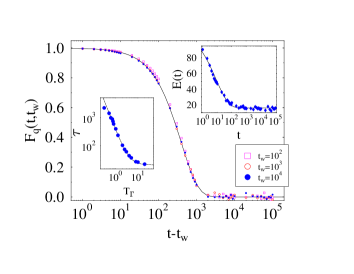
FIG. 1.: Upper inset The energy, $E(t)$, of inherent states as a function of the “tap” number $t$, during a tap dynamics with a tap amplitude $T_{\Gamma}=1.25~{}J$ and tap duration $\tau_{0}=1~{}MCS$, in the Frustrated Lattice Gas of the text. Main frame The self-scattering two times function, $F_{q}(t,t_{w})=\sum_{i}\mbox{e}^{\vec{q}{\cdot}[\vec{r}_{i}(t)-\vec{r}_{i}(t_{w})]}/\rho L^{3}$ as a function of the number $t-t_{w}$ ($T_{\Gamma}=1~{}J$, $\tau_{0}=1~{}MCS$ and $q=\pi/4$). Lower Inset The equilibration time, $\tau$, as a function of $T_{\Gamma}$ (for $\tau_{0}=1~{}MCS$): $\tau$ diverges at low $T_{\Gamma}$. After a transient, $E(t)$ reaches its time independent asymptotic value, and $F_{q}=F_{q}(t-t_{w})$ depends only on the difference of $t-t_{w}$, showing that the system has reached a stationary state (our data are averaged up to $32$ noise realizations).

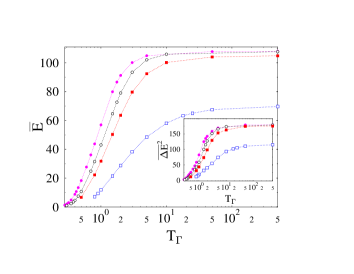
FIG. 2.: The time average of the energy, ${\overline{E}}$, and (inset) its fluctuations, $\overline{\Delta E^{2}}$, recorded at stationarity during a tap dynamics with tap amplitude, $T_{\Gamma}$, in the Frustrated Lattice Gas model. The four different curves correspond to sequences of tap with different values of the duration of each single tap, $\tau_{0}=100,~{}10,~{}5,~{}1~{}MCS$ (from top to bottom).

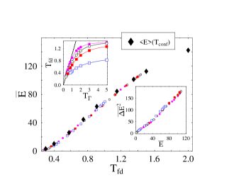
FIG. 3.: Lower Inset The time averages of energy fluctuations, $\overline{\Delta E^{2}}$, when plotted as function of the time average of energy, ${\overline{E}}$, collapse on a single master function for all the different values of tap amplitude and duration, $T_{\Gamma}$ and $\tau_{0}$, shown in Fig.2. Main frame The time average, ${\overline{E}}$, and the ensemble average over the distribution eq.(3), $\langle E\rangle$ (black filled diamonds), plotted respectively as a function of $T_{fd}\equiv\beta^{-1}_{fd}$ and $T_{conf}$, in the Frustrated Lattice Gas model. Upper Inset The temperature $T_{fd}\equiv\beta^{-1}_{fd}$ defined by eq.(2) as function of $T_{\Gamma}$ for $\tau_{0}=100,~{}10,~{}5,~{}1~{}MCS$ (from top to bottom). The straight line is the function $T_{fd}=T_{\Gamma}$.

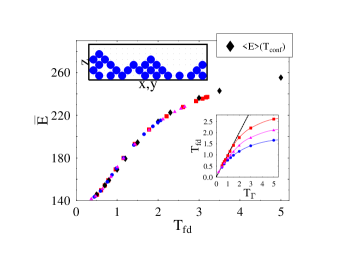
FIG. 4.: Main frame The time average, ${\overline{E}}$, and the ensemble average over the distribution eq.(3), $\langle E\rangle$ (black filled diamonds), plotted respectively as a function of $T_{fd}$ and $T_{conf}$, in the 3D hard-sphere system under gravity described in the text (and schematically depicted in the upper inset). Lower Inset The temperature $T_{fd}\equiv\beta^{-1}_{fd}$ defined by eq.(2) as function of $T_{\Gamma}$ for $\tau_{0}=500,10,5~{}MCS$ (from top to bottom). The straight line is the function $T_{fd}=T_{\Gamma}$.

REFERENCES

- [1] F.H. Stillinger T.A. Weber, Phys. Rev. A 25, 978 (1982). S. Sastry, P.G. Debenedetti, F.H. Stillinger, Nature 393, 554 (1998).
- [2] F. Sciortino, W. Kob, P. Tartaglia, Phys. Rev. Lett. 83, 3214 (1999). F. Sciortino and P. Tartaglia, Phys. Rev. Lett. 86, 107 (2001).
- [3] H.M. Jaeger, S.R. Nagel and R.P. Behringer, Rev. Mod. Phys. 68, 1259 (1996).
- [4] S.F. Edwards and R.B.S. Oakeshott, Physica A 157, 1080 (1989). A. Mehta and S.F. Edwards, Physica A 157, 1091 (1989). S.F. Edwards, in “Disorder in Condensed Matter Physics” page. 148, Oxford Science Pubs (1991); and in Granular Matter: an interdisciplinary approach, (Springer-Verlag, New York, 1994), A. Mehta ed.
- [5] A. Coniglio and M. Nicodemi Physica A 296, 451 (2001).
- [6] A. Barrat, J. Kurchan, V. Loreto and M. Sellitto, Phys. Rev. Lett. 85, 5034 (2000). Phys. Rev. E 63, 051301 (2001).
- [7] J.J. Brey, A. Prados, B. Sánchez-Rey, Physica A 275, 310 (2000); Physica A 284, 277 (2000). A. Prados and J.J. Brey, cond-mat/0106236.
- [8] A. Lefèvre, D. S. Dean, Phys. Rev. Lett. 86, 5639 (2001); cond-mat/0106220.
- [9] J. Berg, S. Franz and M. Sellitto, cond-mat/0111485.
- [10] L. Berthier, L.F. Cugliandolo and J.L. Iguain, Phys. Rev. E 63, 051302 (2001).
- [11] H. A. Makse and J. Kurchan, Nature 415, 614 (2002).
- [12] V. Colizza, A. Barrat and V. Loreto cond-mat/0111458.
- [13] J.B. Knight et al., Phys. Rev. E 51, 3957 (1995).
- [14] J. Berg, A. Mehta, cond-mat/0012416.
- [15] M. Nicodemi, A. Coniglio, H.J. Herrmann, Phys. Rev. E 55, 3962 (1997); J. Phys. A 30, L379 (1997). A. Coniglio and H.J. Herrmann, Physica A 225, 1 (1996).
- [16] A. Coniglio, A. de Candia, A. Fierro, M. Nicodemi, Jour. Phys.: Cond. Mat. 11, A167 (1999).
- [17] A. Coniglio, M. Nicodemi, J. Phys.: Cond. Matt. 12, 6601 (2000); Phys. Rev. Lett. 82, 916 (1999). M. Nicodemi, Phys. Rev. Lett. 82, 3734 (1999).
- [18] J.J. Arenzon, J. Phys. A. 32, L107 (1999).
- [19] is measured in Monte Carlo steps (MCS), where corresponds to attempts to move a particle randomly chosen, and is the number of particles.
- [20] A. Fierro, M. Nicodemi and A. Coniglio, in preparation.