On the Way to a Gutzwiller Density Functional Theory

Abstract

Multi-band Gutzwiller-correlated wave functions reconcile the contrasting concepts of itinerant band electrons versus electrons localized in partially filled atomic shells. The exact evaluation of these variational ground states in the limit of large coordination number allows the identification of quasi-particle band structures, and the calculation of a variational spinwave dispersion. The study of a generic two-band model elucidates the co-operation of the Coulomb repulsion and the Hund’s-rule exchange for itinerant ferromagnetism. We present results of calculations for ferromagnetic nickel, using a realistic 18 spin-orbital basis of $4s$, $4p$ and $3d$ valence electrons. The quasi-particle energy bands agree much better with the photo-emission and Fermi surface data than the band structure obtained from spin-density functional theory (SDFT).

1 Exchange versus Correlations

More than 50 years ago two basically different scenarios had emerged from early quantum-mechanical considerations on electrons in metals with partly filled $d$ bands.

Scenario I:

As proposed by Slater Slaterearly and Stoner Stoner , band theory alone was argued to account for itinerant ferromagnetism. Due to the Pauli principle, electrons with parallel spins cannot come arbitrarily close to each other (“Pauli” or “exchange hole”), and, thus, a ferromagnetic alignment of the electron spins reduces the total Coulomb energy with respect to the paramagnetic situation (“exchange field energy”).

Scenario II:

As emphasized by van Vleck vanVleck , electronic correlations are important in narrow-band materials. Due to the strong electron-electron interaction, charge fluctuations in the atomic $d$ shells are strongly suppressed (“minimum polarity model”). The atomic magnetic moments arise due to the local Coulomb interactions (in particular, Hund’s-rule couplings) and the electrons’ motion through the crystal may eventually align them at low enough temperatures.

In principle, such a dispute can be resolved in natural sciences. The corresponding theories have to be worked out in detail, and their results and predictions have to be compared to experiments.

This was indeed done for scenario I Moruzzi ; thisvolume . The (spin-)density functional theory is a refined band theory which describes some iron group metals with considerable success. Unfortunately, progress for scenario II was much slower. It calls for a theory of correlated electrons, i.e., a genuine many-body problem has to be solved. It was only recently that reliable theoretical tools became available which allow to elucidate scenario II in more detail Nolting ; Hasegawa ; Pruschke ; Vollhardt ; BGWvoll ; correlatedpeople .

A first step in this direction was the formulation of appropriate model Hamiltonians which allowed to discuss matters concisely, e.g., the Hubbard model GutzPRL63 ; Gutzwiller1964 ; Hubbard ; Kanamori . This model covers both aspects of $d$ electrons on a lattice: they can move through the crystal, and they strongly interact when they sit on the same lattice site. The model is discussed in more detail in Sec. 2.

Even nowadays, it is impossible to calculate exact ground-state properties of such a model in three dimensions. In 1963/1964 Gutzwiller introduced a trial state to examine variationally the possibility of ferromagnetism in such a model GutzPRL63 ; Gutzwiller1964 . His wave function covers both limits of weak and strong correlations and should, therefore, be suitable to provide qualitative insights into the magnetic phase diagram of the Hubbard model. Gutzwiller-correlated wave functions for multi-band Hubbard models are defined and analyzed in Sec. 3.

The evaluation of multi-band Gutzwiller wave functions itself poses a most difficult many-body problem. Perturbative treatments Stollhoff ; Carmelo are constrained to small to moderate interaction strengths. The region of strong correlations could only be addressed within the so-called “Gutzwiller approximation” GutzPRL63 ; Gutzwiller1964 ; Vollirev and its various extensions Chao ; Fazekas . Some ten years ago, the Gutzwiller approximation was found to become exact for the one-band Gutzwiller wave function in the limit of infinite spatial dimensions, $d\to\infty$ MVGUTZ ; MVPRLdinfty ; BUCH , and Gebhard Geb1990 developed a compact formalism which allows the straightforward calculation of the variational ground-state energy in infinite dimensions. Recently, Gebhard’s approach was generalized by us to the case of multi-band Gutzwiller wave functions BGWvoll . Thereby, earlier results by Bünemann and Weber BueWeb , based on a generic extension of the Gutzwiller approximation JoergEJB , were found to become exact in infinite dimensions BGWhalb .

As shown in Sect. 4 for a two-band toy model, the Gutzwiller variational scheme approach also allows the calculation of spinwave spectra Buene2000 . In this way, the dispersion relation of the fundamental low-energy excitations can be derived consistently. Albeit the description is based on itinerant electrons, the results for strong ferromagnets resemble those of a Heisenberg model for localized spins whereby a unified description of localized and itinerant aspects of electrons in transition metals is achieved.

In Sect. 5 we discuss results from a full-scale calculation for nickel. The additional local correlations introduced in the Gutzwiller scheme lead to a much better description of the quasi-particle properties of nickel than in previous calculations based on spin-density functional theory.

2 Hamilton Operator

Our multi-band Hubbard model Hubbard is defined by the Hamiltonian

$$\hat{H}=\sum_{i,j;\mathbf{\sigma},\mathbf{\sigma^{\prime}}}t_{i,j}^{\mathbf{\sigma},\mathbf{\sigma^{\prime}}}\hat{c}_{i;\mathbf{\sigma}}^{+}\hat{c}_{j;\mathbf{\sigma^{\prime}}}^{\vphantom{+}}+\sum_{i}\hat{H}_{i;{\rm at}}\equiv\hat{H}_{1}+\hat{H}_{{\rm at}}\;.$$ (1)

Here, $\hat{c}_{i;\mathbf{\sigma}}^{+}$ creates an electron with combined spin-orbit index $\mathbf{\sigma}=1,\ldots,2N$ ($N=5$ for 3$d$ electrons) at the lattice site $i$ of a solid.

The most general case is treated in Ref. BGWvoll . In this work we assume for simplicity that different types of orbitals belong to different representations of the point group of the respective atomic state (e.g., $s$, $p$, $d(e_{g})$, $d(t_{2g})$). In this case, different types of orbitals do not mix locally, and, thus, the local crystal field is of the from $t_{i,i}^{\mathbf{\sigma},\mathbf{\sigma^{\prime}}}=\epsilon_{\mathbf{\sigma}}\delta_{\mathbf{\sigma},\mathbf{\sigma^{\prime}}}$. Consequently, we may later work with normalized single-particle product states $|\Phi_{0}\rangle$ which respect the symmetry of the lattice, i.e.,

$$\langle\Phi_{0}|\hat{c}_{i;\mathbf{\sigma}}^{+}\hat{c}_{i;\mathbf{\sigma^{\prime}}}^{\vphantom{+}}|\Phi_{0}\rangle=\delta_{\mathbf{\sigma},\mathbf{\sigma^{\prime}}}n_{i;\mathbf{\sigma}}^{0}\;.$$ (2)

We further assume that the local interaction is site-independent

$$\hat{H}_{i;{\rm at}}=\sum_{\mathbf{\sigma_{1}},\mathbf{\sigma_{2}},\mathbf{\sigma_{3}},\mathbf{\sigma_{4}}}{\cal U}^{\mathbf{\sigma_{1}},\mathbf{\sigma_{2}};\mathbf{\sigma_{3}},\mathbf{\sigma_{4}}}\hat{c}_{i;\mathbf{\sigma_{1}}}^{+}\hat{c}_{i;\mathbf{\sigma_{2}}}^{+}\hat{c}_{i;\mathbf{\sigma_{3}}}^{\vphantom{+}}\hat{c}_{i;\mathbf{\sigma_{4}}}^{\vphantom{+}}\;.$$ (3)

This term represents all possible local Coulomb interactions.

As our basis for the atomic problem we choose the configuration states

$$|I\rangle=|\mathbf{\sigma_{1}},\mathbf{\sigma_{2}},\ldots\rangle=\hat{c}_{i;\mathbf{\sigma_{1}}}^{+}\hat{c}_{i;\mathbf{\sigma_{2}}}^{+}\cdots|{\rm vacuum}\rangle\quad(\mathbf{\sigma_{1}}<\mathbf{\sigma_{2}}<\cdots)\;,$$ (4)

which are the “Slater determinants” in atomic physics. The diagonalization of the Hamiltonian $\hat{H}_{i;{\rm at}}$ is a standard exercise Sugano . The eigenstates $|\Gamma\rangle$ obey

$$|\Gamma\rangle=\sum_{I}T_{I,\Gamma}|I\rangle\;,$$ (5)

where $T_{I,\Gamma}$ are the elements of the unitary matrix which diagonalizes the atomic Hamiltonian matrix with entries $\langle I|\hat{H}_{i;{\rm at}}|I^{\prime}\rangle$. Then,

$$\hat{H}_{i;{\rm at}}=\sum_{\Gamma}E_{\Gamma}\hat{m}_{\Gamma}\quad,\quad\hat{m}_{\Gamma}=|\Gamma\rangle\langle\Gamma|\;.$$ (6)

The atomic properties, i.e., eigenenergies $E_{\Gamma}$, eigenstates $|\Gamma\rangle$, and matrix elements $T_{I,\Gamma}$, are essential ingredients of our solid-state theory.

3 Multi-band Gutzwiller Wave Functions

3.1 Variational Ground-State Energy

Gutzwiller-correlated wave functions are written as a many-particle correlator $\hat{P}_{{\rm G}}$ acting on a normalized single-particle product state $|\Phi_{0}\rangle$,

$$|\Psi_{{\rm G}}\rangle=\hat{P}_{{\rm G}}|\Phi_{0}\rangle\;.$$ (7)

The single-particle wave function $|\Phi_{0}\rangle$ which obeys (2) contains many configurations which are energetically unfavorable with respect to the atomic interactions. Hence, the correlator $\hat{P}_{{\rm G}}$ is chosen to suppress the weight of these configurations to minimize the total ground-state energy of (1). In the limit of strong correlations the Gutzwiller correlator $\hat{P}_{{\rm G}}$ should project onto atomic eigenstates. Therefore, the proper multi-band Gutzwiller wave function with atomic correlations reads

$$\hat{P}_{{\rm G}} = \prod_{i}\hat{P}_{i;{\rm G}}\;,$$ (8)

$$\hat{P}_{i;{\rm G}} = \prod_{\Gamma}\lambda_{i;\Gamma}^{\hat{m}_{i;\Gamma}}=\prod_{\Gamma}\left[1+\left(\lambda_{i;\Gamma}-1\right)\hat{m}_{i;\Gamma}\right]=1+\sum_{\Gamma}\left(\lambda_{i;\Gamma}-1\right)\hat{m}_{i;\Gamma}\;.$$ (9)

The $2^{2N}$ variational parameters $\lambda_{i;\Gamma}$ per site are real, positive numbers. For $\lambda_{i;\Gamma_{0}}\neq 0$ and all other $\lambda_{i;\Gamma}=0$ all atomic configurations at site $i$ but $|\Gamma_{0}\rangle$ are removed from $|\Phi_{0}\rangle$. Therefore, by construction, $|\Psi_{\rm G}\rangle$ covers both limits of weak and strong coupling. In this way it incorporates both itinerant and local aspects of correlated electrons in narrow-band systems.

The class of Gutzwiller-correlated wave functions as specified in (9) was evaluated exactly in the limit of infinite dimensions in Ref. BGWvoll . The expectation value of the Hamiltonian (1) reads hint

$$\langle\hat{H}\rangle = \frac{\langle\Psi_{\rm G}|\hat{H}|\Psi_{\rm G}\rangle}{\langle\Psi_{\rm G}|\Psi_{\rm G}\rangle}$$ (10)

$$= \sum_{i\neq j;\mathbf{\sigma},\mathbf{\sigma^{\prime}}}t_{i,j}^{\,\mathbf{\sigma},\mathbf{\sigma^{\prime}}}\sqrt{q_{i;\mathbf{\sigma}}}\sqrt{q_{j;\mathbf{\sigma^{\prime}}}}\langle\Phi_{0}|\hat{c}_{i;\mathbf{\sigma}}^{+}\hat{c}_{j;\mathbf{\sigma^{\prime}}}^{\vphantom{+}}|\Phi_{0}\rangle+\sum_{i;\mathbf{\sigma}}\epsilon_{\mathbf{\sigma}}n_{i;\mathbf{\sigma}}^{0}+\sum_{i;\Gamma}E_{\Gamma}m_{i;\Gamma}\;.$$ (11)

Here, $n_{i,\mathbf{\sigma}}^{0}=\langle\Phi_{0}|\hat{n}_{i;\mathbf{\sigma}}|\Phi_{0}\rangle$ is the local particle density in $|\Phi_{0}\rangle$. The local $q$ factors are given by BGWvoll

$$\sqrt{q_{\mathbf{\sigma}}} = \sqrt{\frac{1}{n_{\mathbf{\sigma}}^{0}(1-n_{\mathbf{\sigma}}^{0})}}\sum_{\Gamma,\Gamma^{\prime}}\sqrt{\frac{m_{\Gamma}m_{\Gamma^{\prime}}}{m_{\Gamma}^{0}m_{\Gamma^{\prime}}^{0}}}\sum_{I,I^{\prime}\,(\mathbf{\sigma}\not\in I,I^{\prime})}f_{\mathbf{\sigma}}^{I}f_{\mathbf{\sigma}}^{I^{\prime}}\sqrt{m_{(I^{\prime}\cup\mathbf{\sigma})}^{0}m_{I^{\prime}}^{0}}$$ (13)

$$\hphantom{\sqrt{\frac{1}{n_{\mathbf{\sigma}}^{0}(1-n_{\mathbf{\sigma}}^{0})}}\sum_{\Gamma,\Gamma^{\prime}}}\times T_{\Gamma,(I\cup\mathbf{\sigma})}^{+}T_{(I^{\prime}\cup\mathbf{\sigma}),\Gamma}T_{\Gamma^{\prime},I^{\prime}}^{+}T_{I,\Gamma^{\prime}}\;,$$

where $m_{i;I}^{0}$ ($m_{i;\Gamma}^{0}$) is the probability to find the configuration $|I\rangle$ (the atomic eigenstate $|\Gamma\rangle$) on site $i$ in the single-particle product state $|\Phi_{0}\rangle$. The fermionic sign function $f_{\mathbf{\sigma}}^{I}\equiv\langle I\cup\mathbf{\sigma}|\hat{c}_{\mathbf{\sigma}}^{+}|I\rangle$ gives a minus (plus) sign if it takes an odd (even) number of anticommutations to shift the operator $\hat{c}_{\mathbf{\sigma}}^{+}$ to its proper place in the sequence of electron creation operators in $|I\cup\mathbf{\sigma}\rangle$.

Eqs. (10) and (13) show that we may replace the original variational parameters $\lambda_{i;\Gamma}$ by their physical counterparts, the atomic occupancies $m_{i;\Gamma}$. They are related by the simple equation BGWvoll

$$m_{i;\Gamma}=\lambda_{i;\Gamma}^{2}m_{i;\Gamma}^{0}\;.$$ (14)

The probability for an empty site ($|I|=0$) is obtained from the completeness condition,

$$m_{i;\emptyset}=1-\sum_{\Gamma\,(|\Gamma|\geq 1)}m_{i;\Gamma}\;.$$ (15)

The probabilities for a singly occupied site ($|I|=1$) are given by hint

$$\halign to=433.62pt{\@eqnsel\hskip\@centering$\displaystyle{#}$&\global\@eqcnt\@ne\hskip 2\arraycolsep\hfil${#}$\hfil&\global\@eqcnt\tw@\hskip 2\arraycolsep$\displaystyle{#}$\hfil&\llap{#}\cr\hfil\hskip 0.0pt plus 1000.0pt$\displaystyle{m_{i;\mathbf{\sigma}} &10.0pt\hfil${=&10.0pt$\displaystyle{n_{i;\mathbf{\sigma}}^{0} - \sum_{I \, (|I|\geq 2) \, (\mathbf{\sigma}\in I) } m_{i;I} \;, {}&\hbox to0.0pt{\hss{\rm(0.16a)}\cr\penalty 100\vskip 3.0pt\vskip 0.0pt\cr\hfil\hskip 0.0pt plus 1000.0pt$\displaystyle{m_{i;I} &10.0pt\hfil${=&10.0pt$\displaystyle{\sum_{K} \biggl{|} \sum_{\Gamma} \sqrt{\frac{m_{i;\Gamma}}{m_{i;\Gamma}^{0}}} T_{\Gamma,I}^{+} T_{K,\Gamma} \biggr{|}^{2} m_{i;K}^{0} \; . &\hbox to0.0pt{\hss{\rm(0.16b)}\cr}}}}}}}}}$$

The parameters $m_{i;\emptyset}$ and $m_{i;\mathbf{\sigma}}$ must not be varied independently. All quantities in (10) are now expressed in terms of the atomic multi-particle occupancies $m_{i;\Gamma}$ ($|\Gamma|\geq 2$), the local densities $n_{i;\mathbf{\sigma}}^{0}$, and further variational parameters in $|\Phi_{0}\rangle$.

It is seen that the variational ground-state energy can be cast into the form of the expectation value of an effective single-particle Hamiltonian with renormalized electron transfer amplitudes $\widetilde{t}_{i,j}^{\,\mathbf{\sigma},\mathbf{\sigma^{\prime}}}$,

$$\hat{H}_{\rm eff} = \sum_{i\neq j;\mathbf{\sigma},\mathbf{\sigma^{\prime}}}\widetilde{t}_{i,j}^{\,\mathbf{\sigma},\mathbf{\sigma^{\prime}}}\hat{c}_{i;\mathbf{\sigma}}^{+}\hat{c}_{j;\mathbf{\sigma^{\prime}}}^{\vphantom{+}}+\sum_{i;\mathbf{\sigma}}\epsilon_{\mathbf{\sigma}}\hat{n}_{i;\mathbf{\sigma}}+\sum_{i;\Gamma}E_{\Gamma}m_{i;\Gamma}\,,$$ (17)

$$\widetilde{t}_{i,j}^{\,\mathbf{\sigma},\mathbf{\sigma^{\prime}}} = \sqrt{q_{i;\mathbf{\sigma}}}\sqrt{q_{j;\mathbf{\sigma^{\prime}}}}t_{i,j}^{\,\mathbf{\sigma},\mathbf{\sigma^{\prime}}}\;.$$ (18)

Therefore, $|\Phi_{0}\rangle$ is the ground state of $\hat{H}_{\rm eff}$ whose parameters have to be determined self-consistently from the minimization of $\langle\Phi_{0}|\hat{H}_{\rm eff}|\Phi_{0}\rangle$ with respect to $m_{i;\Gamma}$ and $n_{i;\mathbf{\sigma}}^{0}$. For the optimum set of parameters, $\hat{H}_{\rm eff}^{\rm opt}$ defines a band structure for correlated electrons. Similar to density-functional theory, this interpretation of our ground-state results opens the way to detailed comparisons with experimental results; see Sect. 5.3.

3.2 Spinwaves

The variational principle can also be used to calculate excited states Messiah . If $|\Phi\rangle$ is the ferromagnetic, exact ground state with energy $E_{0}$, the trial states

$$|\Psi(q)\rangle=\hat{S}_{q}^{-}|\Phi\rangle$$ (19)

are necessarily orthogonal to $|\Phi\rangle$, and provide an exact upper bound to the first excited state with momentum $q$ and energy $\epsilon(q)$

$$\epsilon(q)\leq E_{\rm s}(q)\equiv\frac{\langle\Psi(q)|\hat{H}|\Psi(q)\rangle}{\langle\Psi(q)|\Psi(q)\rangle}-E_{0}\;.$$ (20)

Here, $\hat{S}_{q}^{-}=(\hat{S}_{q}^{+})^{+}=\sum_{l,b}\exp(-{\rm i}ql)\hat{c}_{l,b,\downarrow}^{+}\hat{c}_{l,b,\uparrow}^{\vphantom{+}}$ flips a spin from up to down in the system whereby it changes the total momentum of the system by $q$. In this way, the famous Bijl-Feynman formula for the phonon-roton dispersion in superfluid Helium was derived Feynman . In the case of ferromagnetism the excitation energies $E_{\rm s}(q)$ can be identified with the spinwave dispersion if a well-defined spinwave exists at all Buene2000 . Experimentally this criterion is fulfilled for small momenta $q$ and energies $E_{\rm s}(q)$.

Unfortunately, we do not know the exact ground state or its energy in general. However, we may hope that the Gutzwiller wave function $|\Psi_{\rm G}\rangle$ is a good approximation to the true ground state. Then, the states

$$|\Psi_{\rm G}(q)\rangle=\hat{S}_{q}^{-}|\Psi_{\rm G}\rangle$$ (21)

will provide a reliable estimate for $E_{\rm s}(q)$,

$$E_{\rm s}(q)\approx E_{\rm s}^{\rm var}(q)=\frac{\langle\Psi_{\rm G}|\hat{S}_{q}^{+}\hat{H}\hat{S}_{q}^{-}|\Psi_{\rm G}\rangle}{\langle\Psi_{\rm G}|\hat{S}_{q}^{+}\hat{S}_{q}^{-}|\Psi_{\rm G}\rangle}-\frac{\langle\Psi_{\rm G}|\hat{H}|\Psi_{\rm G}\rangle}{\langle\Psi_{\rm G}|\Psi_{\rm G}\rangle}\;.$$ (22)

Naturally, $E_{\rm s}^{\rm var}(q)$ does not obey any strict upper-bound principles.

The actual calculation of the variational spinwave dispersion is rather involved. However, explicit formulae are available Buene2000 which can directly be applied once the variational parameters have been determined from the minimization of the variational ground-state energy.

Figure 1: Phase diagram as a function of $U$ and $J$ for the Hartree–Fock–Stoner theory (HF) and the Gutzwiller wave function (GW) for (a) $n=1.17$ and (b) $n=1.40$; PM: paramagnet, FM: ferromagnet

4 Results for a Generic Two-Band Model

4.1 Ground-State Properties

The atomic Hamiltonian for a two-band model ($b=1,2$) can be cast into the form

$$\hat{H}_{i;{\rm at}} = U\sum_{b}\hat{n}_{b,\uparrow}\hat{n}_{b,\downarrow}+U^{\prime}\sum_{\sigma,\sigma^{\prime}}\hat{n}_{1,\sigma}\hat{n}_{2,\sigma^{\prime}}-J\sum_{\sigma}\hat{n}_{1,\sigma}\hat{n}_{2,\sigma}$$ (24)

$$+J\sum_{\sigma}\hat{c}_{1,\sigma}^{+}\hat{c}_{2,-\sigma}^{+}\hat{c}_{1,-\sigma}^{\vphantom{+}}\hat{c}_{2,\sigma}^{\vphantom{+}}+J_{{\rm C}}\Bigl{(}\hat{c}_{1,\uparrow}^{+}\hat{c}_{1,\downarrow}^{+}\hat{c}_{2,\downarrow}^{\vphantom{+}}\hat{c}_{2,\uparrow}^{\vphantom{+}}+\hat{c}_{2,\uparrow}^{+}\hat{c}_{2,\downarrow}^{+}\hat{c}_{1,\downarrow}^{\vphantom{+}}\hat{c}_{1,\uparrow}^{\vphantom{+}}\Bigr{)}\;.$$

For two $d(e_{g})$ orbitals, $\hat{H}_{{\rm at}}$ exhausts all possible two-body interaction terms. Since we assume that the model describes two degenerate $d(e_{g})$ orbitals, the following restrictions are enforced by the cubic symmetry Sugano : (i) $J=J_{{\rm C}}$, and (ii) $U-U^{\prime}=2J$. Therefore, there are two independent Coulomb parameters, the local Coulomb repulsion $U$ (of the order of $10\,{\rm eV}$) and the local exchange coupling $J$ (of the order of $1\,{\rm eV}$, as typical for atomic Hund’s rule couplings). For the one-particle part $\hat{H}_{1}$ we use an orthogonal tight-binding Hamiltonian with first and second nearest neighbor hopping matrix elements, resulting in a bandwidth $W=6.6\,{\rm eV}$.

In the following we concentrate on two band-fillings, (a), $n=1.17$, where the non-interacting density of states (DOS) shows a pronounced peak at the Fermi energy, most favorably for ferromagnetism, and, (b), $n=1.40$, a position near the DOS peak, where the DOS exhibits a positive curvature as a function of the magnetization.

In Fig. 1 we display the $J$-$U$ phase diagram for both fillings. It shows that Hartree–Fock theory always predicts a ferromagnetic instability. In contrast, the correlated-electron approach strongly supports the ideas of van Vleck vanVleck and Gutzwiller Gutzwiller1964 : (i) a substantial on-site exchange $J$ is required for the occurrence of ferromagnetism if, (ii), realistic Coulomb repulsions $U$ are assumed. At the same time the comparison of Figs. 1a and 1b shows the importance of band-structure effects which are the basis of the Stoner theory. The ferromagnetic phase in the $U$-$J$ phase diagram is much bigger when the density of states at the Fermi energy is large. Therefore, the Stoner mechanism for ferromagnetism is well taken into account in our correlated-electron approach.

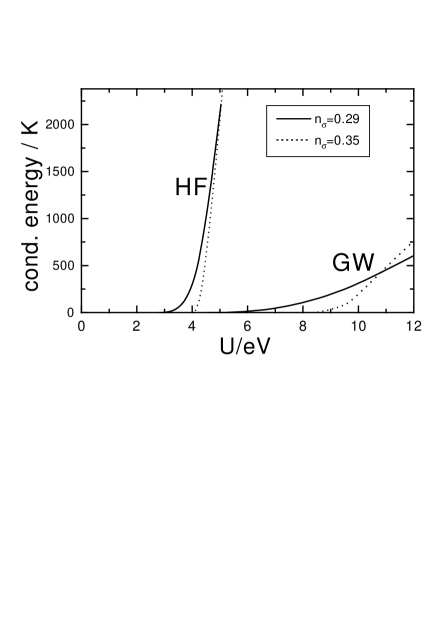
Figure 2: Condensation energy as a function of $U$ for $J=0.2U$ for the Hartree–Fock theory (HF) and the Gutzwiller wave function (GW) for $n=1.17$ (full lines) and $n=1.40$ (dashed lines)

In Fig. 2, we display the energy differences between the paramagnetic and ferromagnetic ground states (“condensation energy”, $E_{\rm cond}$) as a function of the interaction strength for $J=0.2U$. This quantity should be of the order of the Curie temperature which is in the range of $100\,{\rm K}$–$1000\,{\rm K}$ in real materials. The Hartree–Fock–Stoner theory yields such small condensation energies only in the range of $U\approx 4\,$eV; for larger $U$, $E_{\rm cond}$ is of order $U$. In any case, the interaction parameter $U$ has to be tuned very precisely to give condensation energies which concur with experimental Curie temperatures Slaterearly . In contrast, for the Gutzwiller-correlated wave function, we find relatively small condensation energies $E_{\rm cond}=0.5\cdot 10^{3}\,{\rm K}$ even for interaction values as large as twice the bandwidth ($U\approx 12\,$eV). Moreover, the dependence of the condensation energy on $U$ is rather weak such that uncertainties in $U$ do not drastically influence the estimates for the Curie temperature.

4.2 Spinwave Dispersions

In Fig. 3 we show $E_{\rm s}^{\rm var}((q,0,0))$, the variational spinwave dispersion (22), in $x$ direction for the model parameters $n=1.17$, $J=0.2U$, and the four different values $U/{\rm eV}=7.8,10,12,13.6$ which correspond to a magnetization per band of $m=0.12,0.20,0.26,0.28$. This quantity is defined as $0\leq m=(n_{b,\uparrow}-n_{b,\downarrow})/2\leq n/4$. Note that our last case corresponds to an almost complete ferromagnetic polarization. The data fit very well the formula

$$E_{\rm s}^{\rm var}((q,0,0))=Dq^{2}(1+\beta q^{2})+{\cal O}(q^{6})\;,$$ (25)

in qualitative agreement with experiments on nickel nickelexp . The corresponding values $D=1.4\,{\rm eV}\,$Ų and $D=1.2\,{\rm eV}\,$Ų for $m=0.26$ and $m=0.28$, respectively, are of the right order of magnitude for nickel where $D=0.43\,{\rm eV}\,$Ų. As lattice constant of our simple-cubic lattice we chose $a=2.5\,$Å.

Figure 3: Variational spinwave dispersion in $x$ direction, $E_{\rm s}^{\rm var}((q,0,0))$, for the two-band model defined in Sect. 4; $n=1.17$, $J=0.2U$, and the values $U/{\rm eV}=7.8,10,12,13.6$ correspond to $m=0.12,0.20,0.26,0.28$. The lattice constant is $a=2.5\,$Å. Inset: $E_{\rm s}^{\rm var}((q,0,0))$ and $E_{\rm s}^{\rm var}((q/\sqrt{2},q/\sqrt{2},0))$ for $m=0.2$ and $m=0.28$, respectively. The spinwave dispersion is almost isotropic

As shown in the inset of Fig. 3, the dispersion relation is almost isotropic for $q$ values up to half the Brillouin zone boundary Buene2000 , in particular for large magnetizations. This is in contrast to the strong dependence of the electron-transfer amplitudes $t_{i,j}$ on the lattice direction. This implies for strong ferromagnets that the collective motion of the local moments is similar to that of localized spins in an insulator Eschrig . Such ferromagnetic insulators are conveniently described by the Heisenberg model with exchange interactions between neighboring sites $\langle i,j\rangle$ on a cubic lattice,

$$\hat{H}_{\rm S}=-J\sum_{\langle i,j\rangle}\hat{\vec{S}}_{i}\hat{\vec{S}}_{j}\;.$$ (26)

For such a model one finds $D=2SJa^{2}$. The length of the effective local spins can be calculated from $|\Psi_{\rm G}\rangle$ as $S(S+1)\approx 0.95$ ($S=0.6$) for $m\geq 0.20$ BGWvoll . Therefore, $J\approx D/(1.2a^{2})$, which gives the typical value $J=0.17\,{\rm eV}$. For an estimate of the Curie temperature $T_{\rm C}$ we use the result from quantum Monte-Carlo calculations QMCspinmodels

$$T_{\rm C}=1.44JS^{2}$$ (27)

for spins $S$ on a simple-cubic lattice. In this way we find $T_{\rm C}\approx 0.5J=0.09\,{\rm eV}=1\cdot 10^{3}\,{\rm K}$. This is the same order of magnitude as the condensation energy for these values of the interaction, $E_{\rm cond}=5\cdot 10^{2}\,K$, see Sect. 4. Given the arbitrariness in the relation between $E_{\rm cond}$ and $T_{\rm C}$, and the application of the Heisenberg model to our itinerant-electron system, we may certainly allow for difference of a factor two in these quantities. Nevertheless, the results of this section clearly show that, (i), $E_{\rm cond}$ gives the right order of magnitude for $T_{\rm C}$, and that, (ii), the spinwave dispersion of strong itinerant ferromagnets resembles the physics of localized spins.

5 Correlated Band-Structure of Nickel

5.1 Discrepancies Between Experiment and SDFT

Of all the iron group magnetic metals, nickel is the most celebrated case of discrepancies between the results from experiment and from spin-density functional theory (SDFT) Huefner . From very early on, the photo-emission data have indicated that the width of the occupied part of the $d$ bands is approximately $W^{*}_{\rm occ}=3.3\,{\rm eV}$ Eberhardt whereas all SDFT results yield values of $W^{*}_{{\rm occ,SDFT}}=4.5\,{\rm eV}$ or larger Moruzzi ; Eberhardt . Similarly, the low temperature specific heat data Dixon give a much larger value of $N^{*}(E_{\rm F})$, the quasi-particle density of states at the Fermi energy ($3.0$ vs. $1.9$ states/(eV atom)), which indicates a quasi-particle mass enhancement by a factor of approximately $1.6$. Here, the Sommerfeld formula is used to convert the specific heat data; the theoretical value follows directly from the quasi-particle band structure. Furthermore, very detailed photo-emission studies at symmetry points and along symmetry lines of the Brillouin zone show discrepancies to SDFT results for individual band-state energies which are of similar magnitude as seen in the overall $d$ bandwidth.

The studies revealed even bigger discrepancies in the exchange splittings of majority spin and minority spin bands. The SDFT results give a rather isotropic exchange splitting of about $600\,{\rm meV}$ Moruzzi ; Eberhardt ; Callaway . In contrast, the photo-emission data show small and highly anisotropic exchange splittings between $160\,{\rm meV}$ for pure $d(e_{g})$ states such as $X_{2}$ and $330\,{\rm meV}$ for pure $d(t_{2g})$ states, the latter value estimated from the exchange splitting of $\Lambda_{3}$ states along $\Gamma$ to $L$ Donath ; Guenthe . The much larger and much too isotropic exchange splitting of the SDFT results has further consequences.

1. The experimental magnetic moment of the strong ferromagnet Ni is $\mu=0.61\mu_{\rm B}$; yet of relevance is its spin-only part $\mu_{\hbox{\scriptsize spin-only}}=0.55\mu_{\rm B}$ Mook . The SDFT result is $\mu_{\hbox{\scriptsize spin-only}}=0.59\mu_{\rm B}$ Moruzzi , an overestimate related to the too large exchange splitting.

2. the $X_{2}$ state of the minority spin bands lies below $E_{\rm F}$ Hopster , whereas all SDFT results predict it to lie above the Fermi level Moruzzi ; WangCallaway ; Wohlfahrtreview . As a consequence, the SDFT Fermi surface exhibits two hole ellipsoids around the $X$ point of the Brillouin zone whereas in the de-Haas–van-Alphen experiments only one ellipsoid has been found WangCallaway ; Tsui .

3. The strong $t_{2g}$-$e_{g}$ anisotropy is also reflected in the total $d$ hole spin density, i.e., in the observation that the $d$-hole part of the Ni magnetic moment has 81% $d(t_{2g})$ and 19% $d(e_{g})$ character Mook , whereas the SDFT results give a ratio of 74% to 26% Jepsen .

In the late 70’s and early 80’s various authors have investigated in how far many-body effects improve the agreement between theory and experiment, see, e.g., Refs. Cooke ; Liebsch . For example, Cooke et al. Cooke introduced an anisotropic exchange splitting as a fit parameter.

5.2 Present Status of the Gutzwiller-DFT

Limitations:

By construction, the Gutzwiller approach naturally combines with density-functional theory (DFT) which provides a basis of one-particle wave functions and a ‘bare’ band structure. The Gutzwiller-DFT introduces important local correlations and provides a variational ground-state energy, a quasi-particle band structure, and a spin-wave dispersion.

Nevertheless, the Gutzwiller-DFT has its own limitations which we collect here for further reference.

1. It starts from a model Hamiltonian whose parameters need to be determined from a DFT calculation; we shall comment on this procedure below.

2. The true ground state is approximated by a variational many-body wave function; however, our experience from the two-band model supports our hope that the variational freedom of our wave function is big enough to capture the essential features of itinerant ferromagnetism in real materials as well.

3. The variational ground-state energy is evaluated exactly only in the limit of infinite dimensions; however, from the one-band case, we expect $1/d$ corrections to be small Geb1990 .

4. Similar in spirit to density-functional theory, we interpret the ground-state energy in terms of a quasi-particle band structure; it should be kept in mind, though, that this quantity is, in general, not identical to the quasi-particle dispersion in the sense of standard many-body theory FetterWalecka .

5. Most dynamic quantities, e.g., the spectral function, cannot be determined within our approach; the example of the spinwave dispersion in Sect. 4.2 shows, however, that we can calculate low-order moments of spectral functions consistently.

Despite all these restrictions, the method remedies many problems of the SDFT in the description of the quasi-particle band structure of nickel, see Sect. 5.3.

Parameterization of the One-Particle Hamiltonian:

In the present study, we determine the hopping matrix elements $t_{i,j}^{\mathbf{\sigma},\mathbf{\sigma^{\prime}}}$ in (1) from a least squares’ fit to the energy bands obtained from a density-functional-theory calculation for non-magnetic nickel. An orthogonal nine orbital basis is used, and the root-mean-square deviation of the $d$ band energies is about $60\,{\rm meV}$.

A more complete description should include the flexibility of the wave functions to relax in the magnetic state. This could be achieved by enhancing the orbital basis by 4$d$ states. Moreover, spin-orbit coupling is of significance in nickel, as it leads to a 10% enhancement of the total magnetic moment. In principle, the spin-orbit coupling, or, more generally, an arbitrarily large orbital basis can be treated within our formalism BGWvoll , yet it leads to complications such as local $q$ factors which now depend on two spin-orbital indices instead of one as in (13). These extensions not only enhance the numerical complexity of the problem but also require different methods for extracting the single-particle Hamiltonian from DFT, for example by a more direct evaluation of DFT results obtained from local basis methods.

Since we start from a DFT basis, the ‘bare’ band structure incorporates already some important exchange and correlation effects. In particular, we may expect that the non-local Coulomb terms are well taken into account because the electron-electron interaction is screened at a length scale of the order of the inverse Fermi wave number. In this way, we can restrict all explicit Coulomb interaction terms in $\hat{H}$ to local interactions. This assumption is supported by the fact that the Hartree–Fock approximation becomes exact in infinite dimensions for density-density interactions, $\hat{V}^{\mathbf{\sigma},\mathbf{\sigma^{\prime}}}({r\neq 0})=\sum_{l}\hat{n}_{l,\mathbf{\sigma}}\hat{n}_{l+r,\mathbf{\sigma^{\prime}}}\to\hat{V}_{\rm HF}^{\mathbf{\sigma},\mathbf{\sigma^{\prime}}}({r\neq 0})$ MHart . Therefore, we expect that interaction terms beyond the purely local Hubbard interaction should be properly taken into account in the density-functional approach in three dimensions. However, the proper treatment of the “double counting” problem for both local and non-local interactions remains a serious problem for all methods which try to combine density-functional approaches with model-based many-particle theories; see, e.g., the contributions by Lichtenstein, Vollhardt, and Potthoff in this volume.

Chemical Potentials:

In the translationally invariant system under investigation, the local occupation densities are the same as their system averages,

$$\langle\hat{n}_{i,\mathbf{\sigma}}\rangle=\langle\hat{N}_{\mathbf{\sigma}}\rangle/L\;,$$ (28)

where $\hat{N}_{\mathbf{\sigma}}=\sum_{i}\hat{c}_{i;\mathbf{\sigma}}^{+}\hat{c}_{i;\mathbf{\sigma}}^{\vphantom{+}}$ counts the number of electrons with spin-orbit index $\mathbf{\sigma}$. Therefore, we may equally work with chemical potentials $\mu_{\mathbf{\sigma}}$ for each spin-orbit index in the Hamiltonian

$$\hat{H}_{\rm gc}=\hat{H}-\sum_{\mathbf{\sigma}}\mu_{\mathbf{\sigma}}\hat{N}_{\mathbf{\sigma}}\;.$$ (29)

In this grand-canonical view, the chemical potentials rather than the particle densities act as variational parameters. Naturally, not all of these parameters may be varied independently. For example, as a consequence of the hybridization of the 4$sp$ and the 3$d$ electrons, the 3$d$ levels would be depleted for a strong $d$-$d$ repulsion which needs to be compensated using one of the parameters. Presently we keep fixed the values of the 4$s$ and 4$p$ partial charges, and thus also the 3$d$ total charge, to the values of the non-magnetic calculation. This is achieved by using two of the four chemical potentials for 4$s$ and 4$p$ electrons.

As can be seen from (18), the chemical potentials act as a shift of the ‘bare’ (DFT) values of the fields $\epsilon_{\mathbf{\sigma}}$,

$$\epsilon_{\mathbf{\sigma}}^{\rm eff}=\epsilon_{\mathbf{\sigma}}-\mu_{\mathbf{\sigma}}\;.$$ (30)

In this way, the variational approach naturally contains the flexibility to adjust the magnetic (or “exchange”) splitting between majority bands $(b,\uparrow)$ and minority bands $(b,\downarrow)$,

$$\Delta_{b}=\epsilon_{b,{\uparrow}}^{\rm eff}-\epsilon_{b,{\downarrow}}^{\rm eff}\;.$$ (31)

In particular, we may allow for an anisotropy in the exchange splittings of the $d(e_{g})$ and $d(t_{2g})$ electrons.

Interaction Parameters of the Atomic Hamiltonian:

Presently we employ only the on-site Coulomb interaction within the 3$d$ shell, i.e., all interactions within the 4$s$, 4$p$ shell and between 4$sp$ and 3$d$ are neglected. In spherical atom approximation, which is found to be well justified, all matrix elements in (3) can either be expressed as a function of the Slater integrals $F(k)$ ($k=0,2,4$) or of the Racah parameters $A$, $B$, $C$ Sugano . We use $C/B\approx 4$–$5$ Sugano and determine $A$ and $C$ in order to give an optimal agreement with experimental data (effective mass and bandwidth, condensation energy, $t_{2g}/e_{g}$ ratio of the $d$ part of the magnetic moment, Fermi surface topology).

Currently, there is a big debate on the magnitude of the interaction parameters. In principle, the interaction parameters could also be deduced from DFT results. However, there is no consensus on how to calculate these parameters consistently. For example, they could be calculated from atomic or Wannier functions, or they could be found using constrained DFT methods (see, e.g., Ref. Vielsack ).

Minimization:

The number of multi-electron states $|\Gamma\rangle$ is $2^{2N}=2^{10}$. Because of the cubic site symmetry, the number of independent variational parameters $m_{\Gamma}$ reduces to approximately 200 for the paramagnetic and to approximately 400 for the ferromagnetic cases. These “internal” variational parameters obey $2N+1$ sum rules (15) and (3.1); in cubic symmetry there remain three for the paramagnetic and five for the ferromagnetic cases. There is freedom to choose those $m_{\Gamma^{\prime}}$ which, through the sum rules, are dependent on the other $m_{\Gamma}$. It is advisable to pick those $m_{\Gamma^{\prime}}$ which can be expected to have large values. This avoids unphysical negative values of $m_{\Gamma^{\prime}}$ to occur during the variational procedure.

The chemical potentials of (30) are the “external” variational parameters. In the present case these are eight, however three are fixed to yield the total 4$s$, 4$p$, and 3$d$ densities, such that the space of the external parameters is five-dimensional. Given a fixed set of external variational parameters, the procedure to determine the internal ones begins to put them equal to their uncorrelated values $m_{\Gamma}=m^{0}_{\Gamma}$. Thus, $q^{0}_{d,\sigma}=1$. Note that $q_{s,\sigma}=q_{p,\sigma}=1$ always holds, as there is no interaction for 4$s$, 4$p$ orbitals. From this, the ‘bare’ (DFT) band structure and $|\Phi_{0}\rangle^{\rm bare}$ follow as an initial guess for the quasi-particle band structure and one-particle product state. Then, the following self-consistent scheme is employed:

1. Calculate the ground-state energy for $|\Phi_{0}\rangle_{\alpha}^{\rm old}$ where $\alpha$ labels the set of external variational parameters. This requires momentum-space integrations up to the respective Fermi surface.

2. Minimize the ground-state energy (10) with respect to the internal variational parameters.

3. Calculate the $q$ factors and derive $|\Phi_{0}\rangle_{\alpha}^{\rm new}$ as the ground state of the $\hat{H}_{\rm eff}$ (18) with the renormalized hopping matrix elements $\widetilde{t}_{i,j}$; repeat steps 1–3 until convergence to $|\Phi_{0}\rangle_{\alpha}^{\rm opt}$ is reached.

Self-consistency is usually reached rather quickly, i.e., $|\Phi_{0}\rangle_{\alpha}^{\rm opt}$ is found after three to five iterations.

The global minimum, $|\Phi_{0}\rangle_{\rm global}^{\rm opt}$ is found by a search through the space of the external variational parameters keeping the average $d$ and $sp$ occupations. This search can be sped up by first optimizing with respect to the most important external variational parameter which is the isotropic exchange splitting $\Delta_{d}=(\Delta_{e_{g}}+\Delta_{t_{2g}})/2$, putting the difference to zero as a first approximation.

In a second step, the anisotropy of the exchange splitting is investigated, i.e., we introduce $\Delta_{e_{g}}$ and $\Delta_{t_{2g}}$ in the minimization procedure, keeping $\Delta_{d}$ at the value of $\Delta_{d}^{\rm opt}$ obtained in the first optimization step. The searches for $\Delta_{d}^{\rm opt}$, and for $\Delta_{e_{g}}^{\rm opt}$ and $\Delta_{t_{2g}}^{\rm opt}$ can be carried out starting with $|\Phi_{0}\rangle^{\rm bare}$. Only then the self-consistency procedure for $|\Phi_{0}\rangle^{\rm opt}$ has to be launched.

Typical energy gains are (in meV):

$$\halign to=433.62pt{\@eqnsel\hskip\@centering$\displaystyle{#}$&\global\@eqcnt\@ne\hskip 2\arraycolsep\hfil${#}$\hfil&\global\@eqcnt\tw@\hskip 2\arraycolsep$\displaystyle{#}$\hfil&\llap{#}\cr\hfil\hskip 0.0pt plus 1000.0pt$\displaystyle{E_{0}^{\rm bare} - E_{0}^{\rm bare}(\Delta_{d}^{\rm opt}) &10.0pt\hfil${\approx&10.0pt$\displaystyle{\hbox{$10$--$100$} ,{}&\hbox to0.0pt{\hss{\rm(0.32a)}\cr\penalty 100\vskip 3.0pt\vskip 0.0pt\cr\hfil\hskip 0.0pt plus 1000.0pt$\displaystyle{E_{0}^{\rm bare}(\Delta_{d}^{\rm opt}) - E_{0}^{\rm bare}(\Delta_{e_{g}}^{\rm opt},\Delta_{t_{2g}}^{\rm opt}) &10.0pt\hfil${\approx&10.0pt$\displaystyle{\hbox{$5$--$10$} ,{}&\hbox to0.0pt{\hss{\rm(0.32b)}\cr\penalty 100\vskip 3.0pt\vskip 0.0pt\cr\hfil\hskip 0.0pt plus 1000.0pt$\displaystyle{E_{0}^{\rm bare}(\Delta_{e_{g}}^{\rm opt},\Delta_{t_{2g}}^{\rm opt}) - E_{0}^{\rm opt}(\Delta_{e_{g}}^{\rm opt},\Delta_{t_{2g}}^{\rm opt}) &10.0pt\hfil${\approx&10.0pt$\displaystyle{\hbox{$5$--$10$}\; . &\hbox to0.0pt{\hss{\rm(0.32c)}\cr}}}}}}}}}}}}}$$

The energy gains from the variations of $\Delta_{s}$ and $\Delta_{p}$ are of the order of $0.1\,{\rm meV}$.

5.3 Comparison to Experiments

The results for nickel of our DFT-based Gutzwiller calculations agree best with experiment when we choose the following values of the interaction parameters: $A\approx 10$–$12\,{\rm eV}$, $C\approx 0.1$–$0.4\,{\rm eV}$ with $C/B\approx 4.5$ Jubelpaper . The width of the $d$ bands is predominantly determined by $A$ (essentially the Hubbard $U$) via the values of the hopping reduction factors $q_{d,\sigma}$. The exchange splittings and, consequently, the magnetic moment are mainly governed by $C$ and to some extend also by $A$. The Racah parameter $C$ causes the Hund’s-rule splitting of the $d^{8}$ multiplets; in the hole picture, $d^{8}$ is the only many-particle configuration which is significantly occupied (by $1.90$ electrons), while $5.94$ electrons are in $d^{9}$, $0.89$ electrons are in $d^{10}$, and $1.18$ electrons have $s$ or $p$ character.

In our present study, the parameter $C$ is found to be rather small ($0.1\,{\rm eV}$) compared to $A$ in order to reproduce the measured spin-only moment $\mu_{\hbox{\scriptsize spin-only}}=0.55$. Larger values of $C$ move the minimum of the total energy curve $E_{\rm tot}$ vs. magnetization $m$ to values of $m\approx 0.60$–$0.65\mu_{\rm B}$.

There are two points to discuss here. The first concerns the large value of $A$, which seems incompatible with the position of the satellite peak in the photo-emission data at about $6\,{\rm eV}$ below the Fermi energy $E_{\rm F}$ Huefner . Model calculations for this many-body excitation peak use values of $U\approx 3$–$5\,{\rm eV}$. However, these models use single of few $d$ band models, excluding hybridization with the 4$s$, 4$p$ bands, see, e.g., Ref. Liebsch . When, in our calculation, the hybrization effects are switched off, and only the $d$ band contribution to the total energy matters, we also find that values of $A\approx 3$–$5\,{\rm eV}$ agree best with experiment, and $A\approx 10\,{\rm eV}$ would be way out of a reasonable range of parameter values.

The second point concerns the shape of the total energy curve $E_{\rm tot}(m)$ at large values of $m$ in the limit of strong ferromagnetism. In this limit, the increase of the magnetic moment is fed from the $d$ admixture in the majority 4$s$, 4$p$ bands. Compared to analogous curves obtained from SDFT, the curvature at large $m$ values is much smaller in our results. We presume that the larger SDFT curvature is related to the balance between 4$s$, 4$p$ and 3$d$ electrons. It is well known that this balance in a delicate manner determines the stability of transition metals as well as of noble metals; see, e.g., Ref. Pettifor , and the discussion of this problem in Ref. Hafner . The balance between 4$sp$ and 3$d$ electrons is the more influenced the larger the exchange splitting fields are because the minority band 3$d$ level is shifted towards the 4$s$, 4$p$ levels and the majority band 3$d$ level is shifted away. Only in first order of the splitting energy, we can expect that no change in the overall 4$s$, 4$p$ population happens, as is imposed by the choice of our 4$s$, 4$p$ chemical potentials. Presently, the flow between 4$s$, 4$p$ and 3$d$ electrons cannot be described with our model Hamiltonian as the electron-electron interaction within the 4$s$, 4$p$ shell and between 4$sp$ and 3$d$ is not included.

The exchange splittings not only determine the magnetic moment but also influence strongly the shape of the single-particle bands in the vicinity of $E_{\rm F}$ (not the overall bandwidth). For the detailed comparison with photo-emission data we have thus either chosen calculations with small $C$ values ($0.1\,{\rm eV}$), where the minimum of $E_{\rm tot}(m)$ yields $m=0.55\mu_{\rm B}$, or, for larger $C$ values, with a fixed moment constraint, using the experimental spin-only moment of $\mu_{\hbox{\scriptsize spin-only}}=0.55$. The resulting quasi-particle bands do not differ much from each other. There is however a tendency that values $C\approx 0.4\,{\rm eV}$ and larger appear to agree somewhat better with the bulk of the photo-emission data.

Generally, the Gutzwiller results agree much better with experiment than the SDFT results. For example, this is the case for, (i), the value for the quasi-particle density of states at the Fermi energy ($N_{\hbox{\scriptsize G-DFT}}^{*}(E_{\rm F})=2.6$ vs. $3.0$ states/(eV atom)), (ii), the positions of individual quasi-particle energies, (iii), the values of the exchange splittings, (iv), their $t_{2g}$-$e_{g}$ anisotropy, and, (v), the $t_{2g}/e_{g}$ ratio of the $d$ part of the magnetic moment ($(t_{2g}/e_{g})_{\hbox{\scriptsize G-DFT}}=83/17$ vs. $81/19$). As a consequence of the small $d(e_{g})$ exchange splitting, the $X_{2\downarrow}$ state lies below $E_{\rm F}$ and, thus, the Fermi surface exhibits only one hole ellipsoid around $X$, in nice agreement with experiment.

The large anisotropy of the exchange splittings is a result of our ground-state energy optimization, which allows $\Delta_{t_{2g}}$ and $\Delta_{e_{g}}$ to be independent variational parameters. We find $\Delta_{t_{2g}}\approx 3\Delta_{e_{g}}\approx 800\,{\rm meV}$. Note that these values enter $|\Phi_{0}\rangle^{\rm bare}$ and are renormalized by factors $q_{d,\uparrow}\approx 0.7$, $q_{d,\downarrow}\approx 0.6$, when $|\Phi_{0}\rangle^{\rm opt}$ is reached. This also implies that the width of the majority spin bands is about 10% bigger than that of the (higher lying) minority spin bands. It causes a further reduction of the exchange splittings of states near $E_{\rm F}$, especially for those with strong $t_{2g}$ character. Note that this band dispersion effect causes larger exchange splittings near the bottom of the $d$ bands, e.g., $0.45\,{\rm eV}$ splitting of $X_{1}$ and $0.74\,{\rm eV}$ splitting of $X_{3}$. There, however, the quasi-particle linewidths have increased to $1.25\,{\rm eV}$ and $1.4\,{\rm eV}$, respectively Eberhardt , so that an exchange splitting near the bottom of the $d$ bands could, so far, not be observed experimentally.

The large anisotropy may originate from peculiarities special to Ni with its almost completely filled $d$ bands and its fcc lattice structure. Near the top of the $d$ bands, the $t_{2g}$ states dominate because they exhibit the biggest hopping integrals to nearest neighbors, $t^{(1)}_{dd\sigma}\approx 0.5\,{\rm eV}$. The $e_{g}$ states have $t^{(1)}_{dd\pi}\approx-0.3\,{\rm eV}$ to nearest neighbors, and $t^{(2)}_{dd\sigma}\approx 0.1\,{\rm eV}$ to next-nearest neighbors; the latter are small because of the large lattice distance to second neighbors. The $e_{g}$ states also mix with the nearest-neighbor $t_{2g}$ states with $t^{(1)}_{dd\pi}$-type coupling. Therefore, the system can gain more band energy by avoiding occupation of anti-bonding $t_{2g}$ states in the minority spin bands via large values of $\Delta_{t_{2g}}$, at the expense of allowing occupation of less anti-bonding $e_{g}$ states via small $\Delta_{e_{g}}$ values. This scenario should not apply to materials with a bcc lattice structure which have almost equal nearest and next-nearest neighbor separations. Since the bands in nickel are almost completely filled, the suppression of charge fluctuations actually reduces the number of atomic configurations where the Hund’s-rule coupling is active. It is also in this respect that nickel does not quite reflect the generic situation of other transition metals with less completely filled $d$ bands.

The results for nickel presented here must be seen as preliminary inasmuch some important interaction terms were not yet included; see Sect. 5.2. However, the present study already shows that the Gutzwiller-DFT is a working approach. It should allow us to resolve many of the open issues in itinerant ferromagnetism in nickel and other transition metals.

6 Conclusions and Outlook

Which scenario for itinerant ferromagnetism in transition metals is the correct one?

Band theory along the lines of Slater and Stoner could be worked out in much detail whereas a correlated-electron description of narrow-band systems was lacking until recently. Our results for a two-band model and for nickel show that the van-Vleck scenario is valid. Band theory alone does not account for the strong electronic correlations present in the material which lead to the observed renormalization of the effective mass, exchange splittings, bandwidths, and Fermi surface topology. Moreover, charge fluctuations are indeed small, and large local moments are present both in the paramagnetic and the ferromagnetic phases.

Roughly we may say that the electrons’ motion through the crystal leads to a ferromagnetic coupling of pre-formed moments which eventually order at low enough temperatures. In this way, strong itinerant ferromagnets resemble ferromagnetic insulators as far as their low-energy properties are concerned: spinwaves exist which destroy the magnetic long-range order at the Curie temperature.

Our present scheme allows us a detailed comparison with data from refined photo-emission experiments on nickel which are currently carried out Claessen . It should be clear that our approach is applicable not only to nickel but to all other itinerant electron systems.

Despite all recent progress much work remains to be done. The present implementation of the Gutzwiller-DFT needs to be improved by the inclusion of more orbits, their mutual Coulomb interaction terms, and the spin-orbit coupling. Ultimately, some of the principle limitations of our variational approach will have to be overcome by a fully dynamic theory. Most probably, such a theory will require enormous numerical resources such that a fully developed Gutzwiller-DFT will always remain a valuable tool to study ground-state properties of correlated electron systems.

References

- (1) J.C. Slater, Phys. Rev. 49, 537 (1936); ibid., 931 (1936).
- (2) E.C. Stoner, Proc. Roy. Soc. A 165, 372 (1938); for early reviews, see J.C. Slater, Rev. Mod. Phys. 25, 199 (1953) and E.P. Wohlfarth, ibid., 211 (1953).
- (3) J.H. van Vleck, Rev. Mod. Phys. 25, 220 (1953).
- (4) V.L. Moruzzi, J.F. Janak, and A.R. Williams, Calculated Electronic Properties of Metals (Pergamon Press, New York, 1978).
- (5) See also the contributions in this volume by O. Erikson; R. Wu; J. Kübler and K.H. Bennemann; R. Brinzanik; P.J. Jensen.
- (6) W. Nolting, W. Borgieł, V. Dose, and Th. Fauster, Phys. Rev. B 40, 5015 (1989); W. Borgieł and W. Nolting, Z. Phys. B 78, 241 (1990).
- (7) H. Hasegawa, J. Phys. Soc. Jpn 66, 3522 (1997); Phys. Rev. B 56, 1196 (1997); R. Frésard and G. Kotliar, Phys. Rev. B 56, 12909 (1997).
- (8) Th. Obermeier, Th. Pruschke, and J. Keller, Phys. Rev. B 56, 8479 (1997); Th. Maier, M.B. Zölfl, Th. Pruschke, and J. Keller, Euro. Phys. J. B 7, 377 (1999); M.B. Zölfl, Th. Pruschke, J. Keller, A.I. Poteryaev, I.A. Nekrasov, and V.I. Anisimov, Phys. Rev. B 61, 12810 (2000).
- (9) D. Vollhardt, N. Blümer, K. Held, M. Kollar, J. Schlipf, M. Ulmke, and J. Wahle, Adv. in Solid-State Phys. 38, 383 (1999); I.A. Nekrasov, K. Held, N. Blümer, A.I. Poteryaev, V.I. Anisimov, D. Vollhardt, preprint cond-mat/0005207 (2000).
- (10) J. Bünemann, W. Weber, and F. Gebhard, Phys. Rev. B 57, 6896 (1998).
- (11) See also the contributions in this volume by A.I. Lichtenstein; D.M. Edwards and A.C.M. Green; D. Vollhardt; W. Nolting, M. Potthoff, T. Herrmann, and T. Wegner; A.M. Oleś and L.L. Feiner.
- (12) M.C. Gutzwiller, Phys. Rev. Lett. 10, 159 (1963).
- (13) M.C. Gutzwiller, Phys. Rev. 134, A923 (1964); ibid. 137, A1726 (1965).
- (14) J. Hubbard, Proc. Roy. Soc. London Ser. A 276, 238 (1963); ibid. 277, 237 (1964).
- (15) J. Kanamori, Prog. Theor. Phys. 30, 275 (1963).
- (16) G. Stollhoff and P. Fulde, J. Chem. Phys. 73, 4548 (1980); G. Stollhoff and P. Thalmeier, Z. Phys. B 43, 13 (1981); A.M. Oleś and G. Stollhoff, Phys. Rev. B 29, 314 (1984); for further details on the “local ansatz” technique, see P. Fulde, Electron Correlations in Molecules and Solids, Springer Series in Solid-State Sciences 100 (Springer, Berlin, 1991).
- (17) D. Baeriswyl and K. Maki, Phys. Rev. B 31, 6633 (1985); D. Baeriswyl, J. Carmelo, and K. Maki, Synth. Met. 21, 271 (1987).
- (18) D. Vollhardt, Rev. Mod. Phys. 56, 99 (1984).
- (19) K.A. Chao and M.C. Gutzwiller J. Appl. Phys. 42 1420 (1971); K.A. Chao, Phys. Rev. B 4 4034 (1971); ibid. 1088 (1973); J. Phys. C 7 127 (1974).
- (20) P. Fazekas, Lecture Notes on Electron Correlation and Magnetism, Series in Mod. Cond. Matt. Phys. 5 (World Scientific, Singapore, 1999), gives an introduction to the theory of ferromagnetism, and a concise description and some applications of the Gutzwiller approximation.
- (21) W. Metzner and D. Vollhardt, Phys. Rev. Lett. 59, 121 (1987); Phys. Rev. B 37, 7382 (1988).
- (22) W. Metzner and D. Vollhardt, Phys. Rev. Lett. 62, 324 (1989).
- (23) For a review, see F. Gebhard, The Mott Metal-Insulator Transition (Springer, Berlin, 1997).
- (24) F. Gebhard, Phys. Rev. B 41, 9452 (1990).
- (25) J. Bünemann and W. Weber, Phys. Rev. B 55, 4011 (1997).
- (26) J. Bünemann, Eur. Phys. J. B 4, 29 (1998).
- (27) J. Bünemann, F. Gebhard, and W. Weber, J. Phys. Cond. Matt. 8, 7343 (1997).
- (28) J. Bünemann, preprint cond-mat/0005154 (2000).
- (29) S. Sugano, Y. Tanabe, and H. Kamimura, Multiplets of Transition-Metal Ions in Crystals, Pure and Applied Physics 33 (Academic Press, New York, 1970).
- (30) This holds for our symmetry-restricted basis.
- (31) A. Messiah, Quantum Mechanics, 3rd printing (North Holland, Amsterdam, 1965).
- (32) R.P. Feynman, Statistical Mechanics, Frontiers in Physics 36 (Benjamin, Reading, 1972).
- (33) R.D. Lowde and C.G. Windsor, Adv. Phys. 19, 813 (1970).
- (34) See, e.g., S.V. Halilov, H. Eschrig, A.Y. Perlov, and P.M. Oppeneer, Phys. Rev. B 58, 293 (1998).
- (35) K. Chen, A.M. Ferrenberg, and D.P. Landau, Phys. Rev. B 48, 3249 (1993).
- (36) For a review, see S. Hüfner, Photoelectron Spectroscopy (Springer, Berlin, 1995).
- (37) W. Eberhardt and E.W. Plummer, Phys. Rev. B 21, 3245 (1980).
- (38) M. Dixon, F.E. Hoare, T.M. Holden, and D.E. Moody, Proc. R. Soc. A 285, 561 (1965).
- (39) J. Callaway in Physics of Transition Metals, ed. by P. Rhodes (Conf. Ser. Notes 55, Inst. of Physics, Bristol, 1981), p. 1.
- (40) M. Donath, Surface Science Reports 20, 251 (1994).
- (41) K.-P. Kämper, W. Schmitt, and G. Güntherodt, Phys. Rev. B 42, 10696 (1990).
- (42) H.A. Mook, Phys. Rev. 148, 495 (1966).
- (43) R. Raue, H. Hopster, and R. Clanberg, Phys. Rev. Lett. 50, 1623 (1983).
- (44) C.S. Wang and J. Callaway, Phys. Rev. B 15, 298 (1977).
- (45) E.P. Wohlfahrt in Handbook of Magnetic Materials 1, ed. by E.P. Wohlfarth (North Holland, Amsterdam, 1980).
- (46) D.C. Tsui, Phys. Rev. 164, 561 (1967).
- (47) O. Jepsen, J. Madsen, and O.K. Andersen, Phys. Rev. B 26, 2790 (1982).
- (48) J.F. Cooke, J.W. Lynn, and H.L. Davis, Phys. Rev. B 21, 4118 (1980).
- (49) A. Liebsch, Phys. Rev. B 23, 5203 (1981).
- (50) A. L. Fetter and J. D. Walecka, Quantum Theory of Many-Particle Systems (McGraw–Hill, New York, 1971).
- (51) E. Müller-Hartmann, Z. Phys. B 74, 507 (1989); ibid. 76, 211 (1989).
- (52) G. Vielsack and W. Weber, Phys. Rev. B 54, 6614 (1996).
- (53) Some preliminary results can be found in J. Bünemann, F. Gebhard, and W. Weber, Found. Phys. 30 (Dec. 2000).
- (54) D.G. Pettifor, J. Magn. Magn. Mat. 15–18,847 (1980).
- (55) J. Hafner, From Hamiltonians to Phase Diagrams: The Electronic and Statistical Mechanical Theory of Sp-Bonded Metals and Alloys (Springer Series in Solid-State Sciences 70, 1987), pp. 72.
- (56) R. Claessen, private communication (2000).