LU TP 01-23

July 2, 2001

Stability of the Kauffman Model

Sven Bilke and Fredrik Sjunnesson
Complex Systems Division, Department of Theoretical Physics
University of Lund, Sölvegatan 14A, S-223 62 Lund, Sweden
http://www.thep.lu.se/complex/

Abstract:

Random Boolean networks, the Kauffman model, are revisited by means of a novel decimation algorithm, which reduces the networks to their dynamical cores. The average size of the removed part, the stable core, grows approximately linearly with $N$, the number of nodes in the original networks. We show that this can be understood as the percolation of the stability signal in the network. The stability of the dynamical core is investigated and it is shown that this core lacks the well known stability observed in full Kauffman networks. We conclude that, somewhat counter-intuitive, the remarkable stability of Kauffman networks is generated by the dynamics of the stable core. The decimation method is also used to simulate large critical Kauffman networks. For networks up to $N=32$ we perform full enumeration studies. Strong evidence is provided for that the number of limit cycles grows linearly with $N$. This result is in sharp contrast to the often cited $\sqrt{N}$ behavior.

Submitted to Physical Review E

PACS numbers: 02.70.Rr, 05.40.-a, 87.23.Kg, 89.75.Hc

1 Introduction

Boolean networks were introduced by Kauffman [1, 2] as simplified models of the complex interaction in the regulatory networks of living cells. The binary variable $\sigma_{i}$ encodes the activity of the effective “gene” $i$; expressed or not expressed. Depending upon the initial state, the system evolves to one of the several limit cycles. In the biological picture, the different limit cycles are interpreted as different cell types. One of Kauffman’s motivations for investigating these networks was the idea that the structure of genetic networks present in nature is not only determined by selection. Rather, a good fraction of the network functionality is inherent in the ensemble of regulatory networks as such. In fact, he found an ensemble of critical Boolean networks “on the edge of chaos” that captures some features observed in nature. These Boolean networks show a remarkable stability; in most cases small perturbations in the state of the network do not change the trajectory to a different limit cycle. This is desirable in the biological interpretation since stability of genetic regulatory networks against small fluctuations is a crucial property. Another striking observation is that the number of limit cycles for the critical Boolean networks grows as a square-root of the system size [1, 2]. This is an analogy to multicellular organisms, where it is found empirically that the number of cell-types also grows approximately as the square-root of the genome-size.

The model also exhibits analogies [3] with infinite range spin glasses [4]. In the framework of an annealed approximation [5], some of the previous numerical observations concerning a phase transition between a frozen and a chaotic phase in the model could be understood. The average limit Hamming distance $d_{h}$, the number of bit-wise differences between two random configurations, was used as an order parameter. In the frozen phase one has $d_{h}=0$ for infinite systems whereas in the chaotic phase one has $d_{h}\neq 0$. The parameter driving the transition is the probability $p$ that two different inputs to a Boolean variable $\sigma_{i}$ give raise to different values. In [6] the annealed approximation was extended to provide distributions for the number and the length of the limit cycles. Also, good agreement between the results from the annealed approximation and the numerical calculations was demonstrated in the chaotic phase. An alternative order parameter $s$, the fraction of variables that are stable, i.e. evolve to the same fixed state independently of the initial state, was introduced in [7]. In the infinite size limit one has $s=1$ in the frozen phase, whereas $s\neq 1$ in the chaotic phase. In [8] the concept of relevant variables was introduced. A variable $\sigma_{i}$ is not relevant, if it is stable and/or no variable state depends on $\sigma_{i}$. The relevant variables are of interest since they contain all information about the asymptotic dynamics of the network, i.e. the number of limit cycles and their cycle lengths.

In this work we focus on the stability of the Kauffman model and how this property is related to the stable core of the network. The probability that inversion of a single variable will make the system end up in a different limit cycle is known to be small and approaches zero for large networks. However, we find that if the network is reduced to its relevant core, this probability in drastically raised and increases slightly with the system size.

To facilitate this study we introduce a method that removes variables that cannot be relevant by inspection of transition functions and network connectivity. The resulting reduced network contains all relevant variables and possibly some irrelevant ones. Since all relevant variables are included it will have exactly the same asymptotic dynamics as the original network even though the total number of variables is drastically reduced. We find that resulting number of variables is close to the true number of relevant variables. This indicates that properties of the stable core can mostly be understood by the comparatively trivial interactions detected in the decimation procedure.

The decimation procedure can also be used to reduce the bias in the estimate of some observables like for example the number $n_{c}$ of limit cycles. Different from earlier works we do not observe a $\sqrt{N}$ scaling, but rather a linear growth of $n_{c}$ with the system size.

2 The Kauffman Model

A random Boolean network essentially is a cellular automaton with $N$ binary state variables $\sigma_{i}$. These evolve synchronously according to the transition functions $f_{i}(\{\sigma\})$, which are chosen randomly at time $t=0$ and are then kept fixed. In the Kauffman model $f_{i}$ are constrained to depend on at most $K$ different randomly chosen input variables:

$$\sigma_{i}(t)=f_{i}[\sigma_{v_{i}^{1}}(t-1),\ldots,\sigma_{v_{i}^{K}}(t-1)],$$ (1)

for every variable $\sigma_{i}$. The integers $\{v_{i}^{1},\ldots,v_{i}^{K}\}$ define the input connections to variable $i$.

The transition function $f_{i}$ maps each possible combination of input signals to Boolean output values. These output values are independently set to $true$ or $false$ with probabilities $p$ and $1-p$ respectively. This makes some functions independent of some or all of its $K$ input variables. Furthermore, depending on $K$ and $p$, a finite fraction of the state variables $\sigma_{i}$ are not used by any of the transition functions.

The random Boolean network is a deterministic system. Given the state variables at some time, the future trajectory of the $\sigma_{i}$ is known. The volume of the state space is finite, therefore all trajectories must posses a limit cycle. Besides the stability of the system the number of limit cycles, the length distribution of the cycles and transient trajectories are well established observables for this model. In numerical simulations it is in general not possible to probe the models whole state space, except for very small systems. The volume of the $\{\sigma\}$ state space grows exponentially and the number of graphs $\{f_{i}\}$ even super-exponentially. The commonly used strategy for exploring this model therefore contains two approximations.

1. A small fraction of all possible networks is used as a representative ensemble.

2. For each network only a subset of the state space is probed.

Point 2 introduces a systematic bias to the number of limit cycles since not all of them will be found. In the results section we will re-analyze the number of cycles after decimation of irrelevant nodes. This allows full enumeration of state space for up to $N=32$. In this way we get an improved estimate for the scaling of the respective observables with the system size.

3 The Decimation Procedure

It is well known that some variables in a Kauffman network evolve to the same steady state independently of the initial configuration. These stable variables are clearly irrelevant for the asymptotic behavior of the network. The same holds for those variables that do not regulate any other variable, i.e. no transition functions is dependent on them. In fact, as pointed out in [8], for a variable to be relevant it has to be unstable and regulate some unstable variables that in turn regulate others and so on. In other words, a variable is relevant if and only if it is unstable and regulates other relevant variables.

By definition, in the frozen phase the fraction of stable variables goes to unity as $N$ goes to infinity. Therefore, a large fraction of the variables are likely to be stable even for finite $N$. Since the irrelevant variables includes all stable variables, a considerable part of a network does not affect the asymptotic dynamics at all. The process of identifying the irrelevant variables can be divided into two separate steps. Firstly, the stable variables are identified. Secondly, the variables that do not regulate any unstable variables are identified.

Identifying stable variables is in principal easy, but computationally demanding. In [8] this was done by performing simulations of the dynamics of the system and monitoring which variables were in the same state in all probed limit cycles. However, finding all limit cycles essentially means that all $2^{N}$ possible states have to be probed, which is possible only for very small networks. Since a variable that is stable within the probed limit cycles may change state within some of the unprobed limit cycles, searching a fraction of state space will in some cases overestimate number of stable variables.

Here we introduce an alternative method, which by pure inspection of the connectivity and the transition functions of a network identifies variables that must be stable. The basis for our approach is that transition functions dependent on no input variables give a constant output, i.e. the corresponding variable is stable.

As stated above, some transition functions are independent of all their input variables, i.e. they are constants. This means that the corresponding variables will be stable (after the initial time step) and a transition function that is dependent on such variable will receive a constant signal. By replacing the stable input variable with the corresponding constant value, the number of input variables is reduced. For each replaced variable the input state space is reduced by a factor $1/2$ and within this subspace the rule may be independent of yet other input variables. If in the end even this rule become a constant, the corresponding variable is stable (after a transient time), and can be replaced by a constant. Therefore, we have to repeat this procedure until no more stable variables are found. We summerize the method as follows:

1. For every updating function, $f_{i}$, remove all inputs it does not depend upon.

2. For those $f_{i}$ with no inputs, clamp the variable $\sigma_{i}$ to the corresponding constant value.

3. For every $f_{i}$, replace the clamped inputs with the corresponding constant.

4. If any variable has been clamped, repeat from step 1.

For a pseudo-code description of this method see Appendix (A).

Figure 1: $A$ and $B$ have arbitrary but identical updating functions and $C$ implements $xor$. Since $A$ and $B$ also have the same inputs their outputs will be identical. Thus, $C$ will always output $false$, i.e. $C$ is stable and can be removed. $A$ and $B$ are now non-regulating and can be removed too.

It is clear that our method sometimes does not find all stable variables. We see an example of such a situation in Fig. 1. Here the inputs to a function are coupled logically and hereby confined to a subspace of possibilities. Within this subspace the otherwise unstable variable is stable. The figure illustrates just one of the possible couplings between inputs.

Once the stable variables are identified and removed from the network the non-regulating variables can be removed iteratively. Since our method keeps all relevant variables the resulting network will have exactly the same asymptotic dynamics as the original network.

4 Results

Let us start by analyzing the size of the stable core as a function of the system size $N$. In Fig. 2 the the size of the stable core $N^{*}$, identified by the decimation procedure described above, is shown. Each data point is averaged over $10^{4}$ instances of networks. For comparison the size of the stable core $N^{+}$ as estimated by the method used in [8] is also plotted. The latter procedure is based on observations of the dynamics of the full network and identification of nodes acquiring the same constant value independently of the start-configuration. Since only a small part of the state space can be probed in practice, the number $N^{+}$ is biased to overestimate the true size $\eta$ of the stable core. On the other hand, our decimation procedure underestimates $\eta$ because some configurations, like the one depicted in Fig. 1, which may lead to stable variables are not identified. Therefore, we have $N^{+}\leq\eta\leq N^{*}$.

Figure 2: The size of the stable core – the number of variables going to the same constant value independently of the start-configuration – as a function of the network size. The size of the relevant core estimated with our decimation procedure (circle), the observation of the dynamics [8] and Eq. (2) and (3) are in very good agreement.

It is somewhat surprising to observe $N^{+}\approx N^{*}$, which indicates that properties of the stable core can mostly be understood by the comparatively trivial interactions detected in the decimation procedure. The probability $s$ for a node to belong to the stable core can be estimated by using Eq. (2) in [7]

$$s(t+1)=\sum_{k=0}^{K}s(t)^{K-k}(1-s(t))^{k}{K\choose k}p_{k},$$ (2)

where $p_{k}$ is the probability that a transition function for given values of $K-k$ of its input variables is independent of its other $k$ inputs. This equation describes the growth of the stable core with the time. At $t=0$ only nodes which happen to have a constant transition function are stable. At later times non-constant transition functions, which receive inputs from stable nodes, can acquire a constant value. In [7] Eq. (2) was used as a self-consistency equation for infinite systems, i.e. letting $t\to\infty$. In a finite system, the iteration has to stop at some time $T$, which reflects a characteristic length in the network, the maximal distance a signal can flow before it reaches all nodes. The length scale is set by the average distance (in number of links) a signal can travel. The signal pathway in a sparse directed random graph with only a few loops is approximately a branched polymer, where it is known (see e.g. [9]) that the average distance grows polynomial, i.e. $T\sim cN^{\gamma}$. We have fitted the constants $c$ and $\gamma$ numerically to our data and find $\gamma=0.32(3)$.

After removing the $s(T)$ stable nodes, the decimation procedure also eliminates the leaves in the interaction, i.e. those non-constant vertices with out-degree $q(t=0)=0$. This changes the out-degree of the remaining nodes. Therefore, this procedure is repeated until no more nodes with $q(t)=0$ are found. The fraction $P_{l}$ of (indirect) leaves can be estimated by the self consistent equation

$$P_{l}=\sum_{q=1}^{\infty}P(q|\tilde{N},\tilde{K})P_{l}^{q},$$ (3)

where $\tilde{N}=N(1-s)$ is the number of nodes after removing the $\eta$ constant nodes, $\tilde{K}$ is the average in-degree, an $P(q|\tilde{N},\tilde{K})$ the distribution of the out-degree $q$ given in Appendix B. We solved Eq. (2) and (3) numerically, the resulting graph is also shown in Fig. 2, which is in very good agreement with our numerical results.

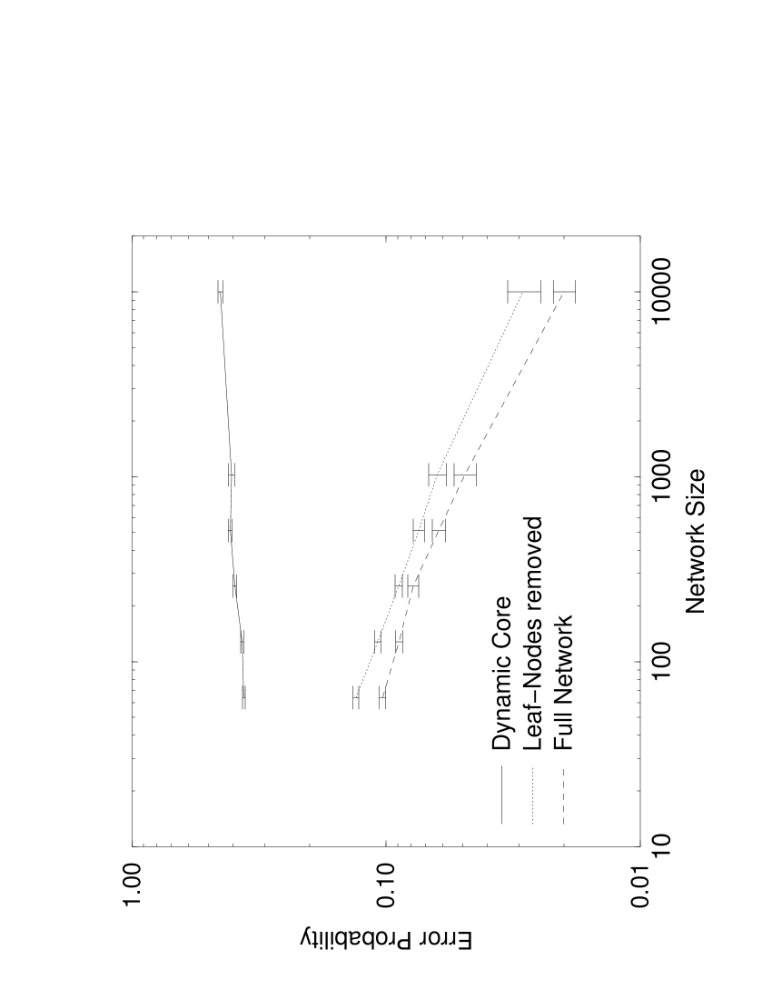
Figure 3: The probability to be pushed out from a limit cycle by the inversion of a randomly chosen variable. For the (full) Kauffman-network (dashed line) the error probability scales to zero for large lattices. This behavior is not changed if one does only a geometric reduction of leaf-variables (dotted line). For the dynamical core (full line) the tolerance against small fluctuations in the state space is completely lost.

One of the important features of Kauffman’s model is the intrinsic stability of critical Boolean networks. How does decimation affect this behavior? While the network reduction does not change the number and the length of limit cycles, the size of the basins of attraction has to be reduced because the state space is shrunken by orders of magnitude. To get a quantitative picture, we analyze the network stability with respect to the inversion of one randomly chosen variable, after the state trajectory has reached a limit cycle. The probability to end up in a different limit cycle compared to the undisturbed system is shown in Fig. 3. If a limit cycle has not been found within $10^{5}$ steps the network is discarded. For the full network we observe the well known stability, the probability to end up in a a different limit cycle asymptotically approaches zero for large lattices. By contrast, for the decimated network the error-probability grows slowly with the network size and the stability is essentially lost. This means, the tolerance against perturbations observed for Kauffman networks is mostly generated by the stable core: in most cases the perturbed signal is “lost” in the stable core and the full network remains unaffected. It has recently been argued [10] that the in-homogeneous, for example scale-free, geometry of real world networks is underlying the stability of these systems. Here we find the opposite: stability is primarily generated dynamically by the propagation (Eq. 2) of the stable core in the network logic. The homogeneous geometry plays only a secondary role: if just a geometric reduction of the network is performed, i.e. the leaf-variables are removed (see the discussion of of Eq. (3)), the error-sensitivity is almost unchanged compared to the full network.

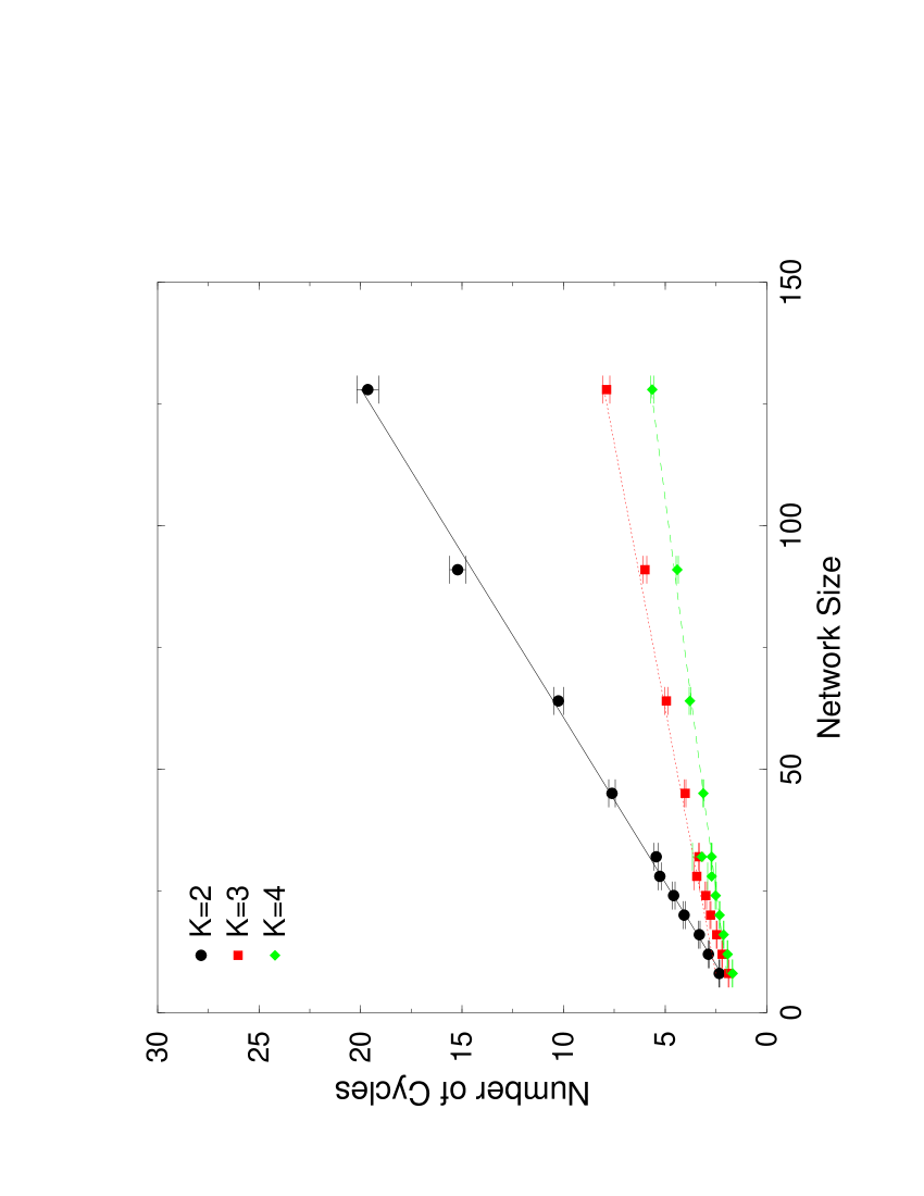
Figure 4: The number of limit cycles as a function of the network size for critical Boolean networks with $K=2,3,4$ inputs. The lines connection the data points are linear interpolations with $\chi^{2}/\mbox{D.O.F}=1.5~{}(K=2),1.6~{}(K=3),1.4~{}(K=4)$. A $\sqrt{N}$ behavior fits the data much worse with $\chi^{2}/\mbox{D.O.F}=11.5~{}(K=2),8.6~{}(K=3),8.5~{}(K=4)$.

The decimation of constant variables from the network enables us to probe a much larger fraction of the state space for a given network. Therefore one may expect to get an better estimate for the number of limit cycles $n_{c}$, which with the commonly used method tends to be underestimated, because some limit cycles may have been missed due to the huge state space. By decimating the networks we can fully enumerate the state space for $N\leq 32$ and hereby get an unbiased estimate. For larger systems we use the standard method with $1000$ restarts on each of the reduced networks. Not unexpectedly we observe a small discontinuity in the curve at the point were the simulation scheme is changed. In Fig. 4 we plot $n_{c}$ as a function of the network size $N$. We do not find the quite often cited $\sqrt{N}$ behavior for this observable. Rather, we find a linear growth with $N$. A possible explanation for the different results obtained in some earlier works may be the bias introduced by the standard method in combination with lower computational power.

5 Summary

The source of the remarkable error tolerance of critical Kauffman model is identified as the “dynamics of the stable core”. While this seems to be a contradiction in terms, it quite nicely describes the percolation-like process, which underlies the propagation of the “stability” signal. Starting from the relatively few nodes with transition functions which do not at all depend on their inputs, the islands of frozen states grow in time by the interaction with the already stable nodes. This process is only limited by the finite size of the system. A small fluctuation in the state of the system will most probably not propagate through the stable core and therefore in most cases has no effect. We demonstrate this by reducing given random networks to the dynamical core, where most of the stable, irrelevant variables have been removed. The stability against small fluctuations for these networks is reduced by orders of magnitude and will probably go to zero for infinite networks. It is interesting to observe that these effects are mostly driven by the network logic and not by the network geometry.

For the identification of the dynamical core we have developed a decimation procedure, which is based on inspection of the networks connectivity and logic. The relatively simple procedure works surprisingly well. The results for the size of the stable core are in very good agreement with the values obtained by observing the dynamics of state-space trajectories in the full network [8].

As a by-product we use the reduced networks to get an improved estimate for the number of limit cycles as a function of the network size. We find that the number of limit cycles grows linearly with $N$, which is in sharp contrast to the square-root behavior reported by other groups. Even though this $\sqrt{N}$ behavior was an interesting analogy with multi-cellular organisms (with approximately $\sqrt{N}$ different cell types for genomes with genome size $N$), our result does in no way reduce the importance of Kauffman networks as an example of self-organized order.

Acknowledgments: We have benefitted from discussions with C. Peterson. This work was in part supported by the Swedish Foundation for Strategic Research and the Knut and Alice Wallenberg Foundation through the SWEGENE consortium.

Appendix A Pseudo Code of the Decimation Procedure

We remind ourselves of the definition of the Kauffman model. $\sigma_{i}(t)$ denotes the state of variable $i$ at time $t$ which is determined by $\sigma_{i}(t)=f_{i}[\sigma_{v_{i}^{1}}(t-1),\ldots,\sigma_{v_{i}^{K}}(t-1)]$ with $\{v\}_{i}=\{v_{i}^{1},\ldots,v_{i}^{K}\}$ defining the connectivity of the network.

We represent the network with a number of nodes, each containing an updating function $f_{i}$ and the list of nodes sending it signals $\{v\}_{i}$. The function decimate reduces the network $Net$ to its relevant core by first removing the stable variables and then those variables that do not regulate any variable.

$node_{i}=[f_{i},\{v\}_{i}]$ $Net=\{node_{1},\dots,node_{N}\}$ decimate($\mathit{Net}$) $\mathbf{do}$ $\mathit{oldNet}$ := $\mathit{Net}$ $\mathbf{for}$ each $\mathit{n}$ $\in$ $\mathit{Net}$ $\mathbf{do}$ remove_unused_inputs($\mathit{n}$, $\mathit{Net}$) remove_if_no_inputs($\mathit{n}$, $\mathit{Net}$) $\mathbf{while}$ $\mathit{oldNet}$ $\neq$ $\mathit{Net}$ $\mathbf{do}$ $\mathit{oldNet}$ := $\mathit{Net}$ $\mathbf{for}$ each $\mathit{n}$ $\in$ $\mathit{Net}$ $\mathbf{do}$ remove_if_no_outputs($\mathit{n}$, $\mathit{Net}$) $\mathbf{while}$ $\mathit{oldNet}$ $\neq$ $\mathit{Net}$ remove_unused_inputs($\mathit{n}$, $\mathit{Net}$) $\mathbf{for}$ each $\mathit{i}$ $\in$ $\mathit{\{v\}_{n}}$ $\mathbf{do}$ $\mathit{flag}$ := $\mathsf{true}$ $\mathbf{for}$ each configuration of inputs $\mathbf{do}$ $\mathbf{if}$ flipping $\mathit{\sigma_{i}}$ changes outcome of $f_{n}$ $\mathbf{then}$ $\mathit{flag}$ := $\mathsf{false}$ $\mathbf{if}$ $\mathit{flag}$=$\mathsf{true}$ $\mathbf{then}$ replace $\mathit{\sigma_{i}}$ with constant value $\mathsf{true}$ in $f_{n}$ remove $\mathit{i}$ from $\mathit{\{v\}_{n}}$ remove_if_no_inputs($\mathit{n}$, $\mathit{Net}$) $\mathbf{if}$ $\mathit{\{v\}_{n}}$=$\emptyset$ $\mathbf{then}$ $\mathbf{for}$ each $\mathit{m}$ with $\mathit{n}$ $\in$ $\mathit{\{v\}_{m}}$ $\mathbf{do}$ replace $\mathit{\sigma_{n}}$ with constant value $f_{n}(\emptyset)$ in $f_{m}$ remove $\mathit{n}$ from $\mathit{\{v\}_{m}}$ remove_if_no_outputs($\mathit{n}$, $\mathit{Net}$) $\mathbf{if}$ $\mathit{n}$ $\notin$ $\mathit{\{v\}_{m}}$ for every $\mathit{m}$ $\mathbf{then}$ remove $\mathit{n}$ from $\mathit{Net}$

Appendix B In- and Out-degree distribution

The reduced number $\tilde{K}$ of inputs after the decimation described in Eq. (2) is the expectation value of the in-degree for the number of inputs from a non-stable variable:

$$\tilde{K}=\frac{1(1-s(T))+2(1-s(T))^{2}}{1-s(T)}=1+2(1-s(T)).$$ (B.4)

The out-degree distribution for a node in the random network can be understood by enumerating the number of ways the $NK$ links can be distributed over this node and the $N-1$ remaining nodes, weighted by the corresponding probabilities to choose the nodes:

$$P(q|N,K)=\left(\frac{1}{N}\right)^{q}\left(\frac{N-1}{N}\right)^{NK-q}{{NK}\choose q}.$$ (B.5)

References

- [1] S. A. Kauffman, J. Theor. Biol. 22, 437 (1969).
- [2] S. A. Kauffman, The Origins of Order (Oxford University Press, 1993).
- [3] B. Derrida and H. Flyvbjerg, J. Phys. A: Math. Gen. 19, L1003 (1986).
- [4] M. Mezard, G. Parisi and M. A. Virasoro, Spin Glass Theory and Beyond (World Scientific, Singapore, 1987).
- [5] B. Derrida and Y. Pomeau, Biophys. Lett. 1, 45 (1986).
- [6] U. Bastolla and G. Parisi, Physica D 98, 1 (1996).
- [7] H. Flyvbjerg, J. Phys. A: Math. Gen. 21, L955 (1988).
- [8] U. Bastolla and G. Parisi, Physica D 115, 203 (1998).
- [9] J. Ambjørn, B. Durhuus, T. Jonsson, Quantum Geometry (Cambridge University Press, 1997).
- [10] H. Jeong, S. P. Mason, Z. N. Oltvai, A.-L. Barabasi, Nature 407, 651 (2000).