Atom laser divergence

Abstract

We measure the angular divergence of a quasi-continuous, rf-outcoupled, free-falling atom laser as a function of the outcoupling frequency. The data is compared to a Gaussian-beam model of laser propagation that generalizes the standard formalism of photonic lasers. Our treatment includes diffraction, magnetic lensing, and interaction between the atom laser and the condensate. We find that the dominant source of divergence is the condensate-laser interaction.

A dilute gas of atoms condensed in a single quantum state of a magnetic trap cornell ; ketterle ; hulet ; kleppner ; hebec ; gasou is the matter-wave analog of photons stored in an optical cavity. A further atomic parallel to photonics is the “atom laser” mewes ; anderson ; hagley ; bloch , a coherent extraction of atoms from a Bose-Einstein condensate. Atom lasers are of basic interest as a probe of condensate properties 2laser and as a coherent source of atoms fringe . Furthermore, just as optical lasers greatly exceeded previous light sources in brightness, atom lasers will be useful in experiments that simultaneously require monochromaticity, collimation, and intensity, such as holographic atom lithography shimizu , continuous atomic clocks clocks , and coupling into atomic waveguides wgload .

Initial work on atom lasers has demonstrated several types of coherent, pulsed output couplers mewes ; anderson ; hagley as well as a coherent narrow-band coupler bloch ; narrowband , which is the type employed in our work. In this Letter, we address the nature of propagation of an atom laser outcoupled from a condensate. Our experimental data show that the laser beam is well characterized by a divergence angle. We measure this angle versus radio-frequency (rf) outcoupler frequency, which chooses the vertical extraction point of the atom laser from the condensate (see Fig. 1a). In choosing the extraction point, one chooses the thickness of the condensate to be crossed by the extracted atoms, as well as the width of the atom laser beam at the extraction plane. To interpret this data, we use a formalism that generalizes the ABCD matrices treatment of photonic lasers kogelnik ; borde . This treatment allows us to calculate analytically the divergence of the laser due to diffraction, magnetic lensing, and interactions with the condensate. We find that, for our typical experimental conditions, the divergence of the laser is primarily due to interaction between the atoms in the laser and the atoms remaining in the condensate. We describe this interaction as a thin lens. Note that the existence of such an interactive lensing effect is in stark contrast to a photonic laser, since photons do not interact. Interactions were estimated to be similarly important for pulsed atom lasers mewes ; hagley . In our case, the divergence is also magnified by a thick-lens-like potential due to the quadratic Zeeman effect of the magnetic trapping fields.

The technique we use to obtain Bose-Einstein condensates with ⁸⁷Rb is described in detail elsewhere orsayBEC . Briefly, a Zeeman-slowed atomic beam loads a MOT in a glass cell. Typically 10⁸ atoms are transferred to a magnetic trap, which is subsequently compressed to oscillation frequencies of $\omega_{x}=\omega_{z}=2\pi\times 144$ Hz and $\omega_{y}=2\pi\times 9$ Hz$=\lambda\omega_{z}$ in the quadrupole and dipole directions, respectively, where $\mathbf{z}$ is vertical. The Ioffe-Pritchard trap is created with an iron-core electromagnet, with a typical quadrupole gradient of 11.7 T$\cdot$m^-1, and an uncompensated dipole bias field of $B_{0}=$5.4 mT. A 40 s, rf-induced evaporative cooling ramp in the compressed trap results in condensates of typically $5\times 10^{5}$ atoms, with a 15% rms shot-to-shot variation.

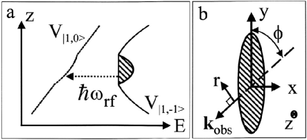
Figure 1: (a) Schematic representation of outcoupling from the trap potential $V_{\left|1,-1\right\rangle}$ to the untrapped $V_{\left|1,0\right\rangle}$ potential via an rf photon at $\omega_{\rm rf}$. The vertical direction is ${\mathbf{z}}$. The curves shown include magnetic, gravitational, and mean field potentials. (b) The wave-vector ${\bf k}_{\rm obs}$ for the absorptive imaging light beam at an angle $\phi$ with respect to the weak axis ${\bf y}$ of the condensate. The horizontal coordinate in the imaging plane is $r$. In both images, the condensate is cross-hatched.

Atom lasers are created by applying a rf field at about 38.6 MHz, to transfer condensate atoms from the trapped $|F,m_{F}\rangle=|1,-1\rangle$ state to the weakly anti-trapped $|1,0\rangle$ state, which also falls under gravity (see Fig. 1a). The rf field is weak (approximately 0.1 $\mu$T) and applied for a relatively long duration ($t_{\rm{oc}}=10$ ms) narrowband . There is no significant coupling to the $|1,+1\rangle$ state because the $F=1$ sublevel transitions are split by 0.8 MHz due to the nonlinear part of the Zeeman effect at 5.4 mT. To measure the spatial distribution of the atom laser, we take an absorptive image with a pulse of resonant light 6 ms after the moment when the rf outcoupling ends and the trap is turned off. As depicted in Fig. 1b, the image is taken at a $\phi=55^{\circ}$ angle from the weakly confining $\mathbf{y}$ axis of the trap. Figure 2a shows a typical image of an atom laser.

The gravitational sag $g/\omega_{z}^{2}$ shifts the entire condensate from the center of the magnetic trap to a region where iso-field surfaces are approximately planes of constant height $z_{0}$ across the condensate bloch . The relation between rf frequency $\omega_{0}+\delta_{\rm{rf}}$ and coupling height $z_{0}$ is

$$\delta_{\rm rf}=-\Delta\frac{z_{0}}{R_{z}}-\frac{\mu}{\hbar}\left(1-\frac{z_{0}^{2}}{R_{z}^{2}}\right)$$ (1)

where $\Delta=MgR_{z}/\hbar$ is the spectral half-width of the condensate, $M$ is the mass of the atom, $g$ is gravitational acceleration, and $R_{z}$ is the Thomas-Fermi (TF) radius dalfovo of the condensate along $\mathbf{z}$. The radius $R_{z}$ is $\sqrt{2\mu/M\omega_{z}^{2}}$, and $\mu$ is the chemical potential $(\hbar\bar{\omega}/2)(15a_{11}N)^{2/5}(M\bar{\omega}/\hbar)^{-1/5}$, where $N$ is the number of atoms in the condensate, $a_{11}=5.67$ nm is the s-wave scattering length between ⁸⁷Rb atoms in the $|1,-1\rangle$ state hall , and $\bar{\omega}^{3}=\omega_{x}\omega_{y}\omega_{z}$. In Eq. (1), we have chosen $\omega_{0}$ such that $\delta_{\rm rf}=\pm\Delta$ when $z_{0}=\mp R_{z}$. For our experimental parameters, $\mu/\hbar\ll\Delta$, so $\delta_{\rm rf}$ is roughly linearly dependent on $z_{0}$, with slope $-Mg/\hbar$. Therefore, in choosing the coupling frequency, we choose the height within the condensate at which the laser is sourced.

Short-term (ms-scale) stability of the bias field is verified by the continuity of flux along the laser (Fig. 2a). We find that the shot-to-shot stability and reproducibility of the bias field, between each 80 s cycle of trapping, cooling, and condensation, is about $\pm 0.4$ $\mu$T or $\pm 3$ kHz. This stability is sufficient to scan through the condensate spectral width of about 20 kHz. In one out of five runs (a run is a set of about 10 cycles), the data were not self-consistent, which we attribute to a larger ($>$1 $\mu$T) bias field fluctuation during that run. We could maintain this bias field stability, typically one part in $10^{4}$ yoke , by using either a low-noise power supply or a battery, since only 1.3 A is used to energize the dipole coils during evaporation and outcoupling.

We analyze the images (such as Fig. 2a) to measure the flux and divergence of the outcoupled laser. Figures 2b through 2d shows the first step in the analysis, a series of fits to the transverse spatial profile of the laser, as measured at several heights $z_{n}$, averaging across $\pm 140$ $\mu$m. The column density profile is fit at each $z_{n}$ by $\rho_{n}(1-r^{2}/R_{n}^{2})^{3/2}$, where $r$ is the horizontal coordinate in the image plane (see Fig. 1b), $\rho_{n}$ is the peak column density, and $R_{n}$ is the width. This fit function would be the rigorously correct function for an atom laser without divergence gerbier or for a free condensate undergoing mean field expansion profile ; here, we observe empirically that the fits are good. From the integral of the column densities at each height, we determine the output flux $F$ with a fit to $F/\sqrt{2g(z-z_{0})}$, a form that assumes constant flux, purely gravitational acceleration, and a density that decreases with the inverse of the classical velocity, valid when $\left|z-z_{0}\right|\gg\ell_{g}$, where $\ell_{g}=[\hbar^{2}/(2gM^{2})]^{1/3}$ is the gravitational length. Finally, from the series $\{R_{n}\}$ and $\{z_{n}\}$, we determine a geometric expansion angle by a linear fit (see Fig. 2e). We will discuss below why one would expect a linear rather than parabolic shape for a laser falling under gravity.

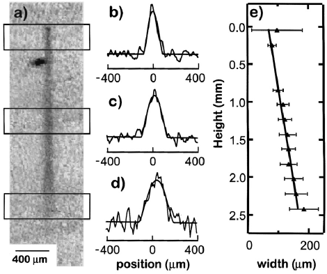
Figure 2: Typical continuous atom laser output. (a) Absorptive image of laser, after 10 ms of output coupling at 38.557 MHz and 6 ms of free flight. The condensate (the darkest area of image) is displaced from the beginning of the laser because of a magnetic kick separating atoms in the $m_{F}=-1$ and $m_{F}=0$ states. (b)–(d) Examples of absorption profiles of the atom laser, taken from the three regions boxed in (a). Each profile is fit to find a width $R_{n}$ and density $\rho_{n}$. (e) The divergence angle of a single laser is found with a linear fit to the series of measured widths $\{R_{n}\}$.

We repeated the above imaging, and analysis for atom lasers coupled at a variety of rf coupling frequencies. Figure 3 shows the averaged half-angle divergence versus outcoupler detuning, from 15 laser images. We see that the divergence clearly decreases at higher $\delta_{\rm{rf}}$, corresponding to lower initial heights $z_{0}$. These divergence data will be analyzed in more detail below. The inset of Fig. 3 shows laser flux $F$ versus $\delta_{\rm{rf}}$, and is compared to

$$\frac{F}{F_{0}}=\left(1-\frac{z_{0}^{2}}{R_{z}^{2}}\right)^{2}\left[1-\frac{2\mu}{\hbar\Delta}\frac{z_{0}}{R_{z}}+\frac{2\mu^{2}}{3\hbar^{2}\Delta^{2}}(1-\frac{z_{0}^{2}}{R_{z}^{2}})\right],$$ (2)

where $F_{0}$ is the peak flux, and Eq. (1) defines the relation between $z_{0}$ and $\delta_{\rm rf}$. Equation (2) assumes the laser flux is simply proportional to the linear density of the condensate at the coupling point. For the solid curve shown in the inset of Fig. 3, we have used $N=4\times 10^{5}$ to give $\Delta=2\pi\times 9.1$ kHz and $R_{z}=4.2$ $\mu$m. The peak flux is measured to be about $1\times 10^{7}$ s^-1 by the reduction in condensate number, as in bloch . This is in agreement with the theory of gerbier , given the applied field strength and uncertainty in the atom number and field polarization narrowband .

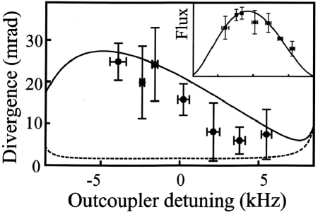
Figure 3: Divergence (half-angle) versus output coupler detuning from the condensate center. Experimental points are compared with the theoretical calculation (solid line). The dashed line represents the same calculation, but excluding the effects of the condensate-laser interaction. Inset: Output flux (in arbitrary units) versus detuning, with the same frequency scale as the main figure.

There are several possible sources of divergence of the atom laser, including diffraction, magnetic lensing, and interactions both within the laser and between the laser and the condensate. In order to understand the divergence with a simple analytical model, we make several approximations: 1) that the interactions between atoms within the laser are not significant, valid in the low-flux limit; 2) that the roughly parabolic density profile of the atom laser can be approximated by a Gaussian; and 3) that we can use stationary solutions of the Schrödinger Equation with a paraxial-type of approximation, in which the fast degrees of freedom gerbier are decoupled from the slow evolution of the transverse degrees of freedom, as in wallis . We follow a Gaussian optics treatment similar to that of photonic lasers kogelnik : the spatial distribution in $\mathbf{x}$ and $\mathbf{y}$ described by the wavefunction $\Psi(x,y,t)=\Psi_{0}\exp{\left[-iP(t)+ix^{2}/2q_{x}(t)+iy^{2}/2q_{y}(t)\right]}$, where $P(t)$ describes the overall phase and amplitude, and beam parameters $1/q_{x,y}(t)=i/w^{2}_{x,y}(t)+c_{x,y}(t)$ describe the widths $w_{x}$ and $w_{y}$ and curvatures $c_{x}$ and $c_{y}$ of the beam. The observable width is $w(t)=(w^{2}_{x}(t)\cos^{2}{(\phi)}+w^{2}_{y}\sin^{2}{(\phi)})^{1/2}$, where $\phi$ is the observation angle (Fig. 1b). The initial widths $w_{x}^{2}(0)=2(R_{z}^{2}-z_{0}^{2})/5$ and $w_{y}(0)=w_{x}(0)/\lambda$ give the same rms width as would an initial Thomas-Fermi density profile.

The beam parameters $q_{x}$ and $q_{y}$ follow an “ABCD law” similar to that for an photon laser beam: $q^{\prime}=(Aq+B)/(Cq+D)$, where the coefficients $A$, $B$, $C$, and $D$ are the four elements in a matrix which transform ray vectors $\langle x,p/\hbar\rangle$ to $\langle x^{\prime},p^{\prime}/\hbar\rangle$ according to classical equations of motion in the same potential. In the following paragraphs, we will calculate the ABCD matrices for interaction with the condensate, propagation with the magnetic trap on, and free flight after the trap is turned off. Note that even though the ray matrices can be derived using classical equations of motion, their application in the Gaussian beam formalism includes diffraction.

The mean-field interaction potential between an atom in the laser and the condensate is $U_{I}({\mathbf{r}})=g_{01}\rho_{c}({\mathbf{r}})$, where $g_{01}$ is the s-wave coupling strength $4\pi\hbar^{2}a_{01}/M$ between atoms in the $|1,0\rangle$ state and the trapped $|1,-1\rangle$ state, and $\rho_{c}({\mathbf{r}})$ is the condensate density. Here we use $a_{01}=a_{11}$. We calculate the action of this potential treating it as a lens, and using the thin lens approximation that each trajectory is at its initial transverse position $\left\langle x_{0},y_{0}\right\rangle$. In the Thomas-Fermi limit, the potential $U_{I}({\mathbf{r}})$ is quadratic, and thus gives an impulse $\left\langle\Delta p_{x},\Delta p_{y}\right\rangle=\left(2\mu\,t_{1}(x_{0},y_{0})/R_{z}^{2}\right)\left\langle x_{0},\lambda^{2}y_{0}\right\rangle$ after an interaction time $t_{1}$. The on-axis power of the lens is given for $x_{0}\ll R_{x}$ and $y_{0}\ll R_{y}$, with which assumption we find $t_{1}^{2}\approx 2(R_{z}+z_{0})/g$. This gives the thin lens ABCD matrix for the $\mathbf{x}$ direction

$$M_{1x}(z_{0})=\left(\begin{array}[]{cc}1&0\\ \frac{2\mu}{\hbar R_{z}^{2}}\sqrt{2(R_{z}+z_{0})}&1\end{array}\right).$$ (3)

When applied to the beam parameter $q_{x}$, the nontrivial term in Eq. (3) is the wavefront curvature added to the beam. A similar ray matrix $M_{1y}(z_{0})$ transforms $q_{y}$, but with a curvature term multiplied by $\lambda^{2}$. For both $M_{1x}(z_{0})$ and $M_{1y}(z_{0})$, the curvature is positive for all $z_{0}$, since the interaction is always repulsive. A positive curvature corresponds to an expanding wave, and thus the condensate with repulsive interactions ($g_{01}>0$) is always a diverging lens.

When the atom laser falls qzesplit , it evolves in the anti-trapping potential due to the quadratic Zeeman effect of the $|1,0\rangle$ state, $U_{\rm QZE}({\mathbf{r}})=-\mu_{B}B^{2}({\mathbf{r}})/B_{\rm HF}$, where $\mu_{B}$ is the Bohr magneton, and $B_{\rm HF}=0.4883$ T is the hyperfine splitting in magnetic units. We can neglect $y$-dependent and higher-order terms, since they are several orders of magnitude smaller for the fields in our experiment, to get $U_{\rm QZE}({\mathbf{r}})\approx-\mu_{B}B_{0}^{2}/B_{\rm HF}-M\Omega^{2}(x^{2}+z^{2})/2$, where $\Omega=2\pi\times 30.3\pm 0.1$ Hz. Below, we will return to evolution in ${\mathbf{y}}$. The classical motion of a particle in an inverted quadratic potential is given by hyperbolic functions. In the vertical direction, an elongation of the laser is evident: we observe a length of 1.84$\pm$0.09 mm, while with gravity alone, one would expect a length of 1.33 mm after 10 ms of coupling and 6 ms of free flight. Including $U_{\rm QZE}({\mathbf{r}})$ and our measured trap parameters, we calculate 1.87 mm, in agreement with our observations. The ray matrix for the transverse $\mathbf{x}$ direction is

$$M_{2}(t_{2})=\left(\begin{array}[]{cc}\cosh(\Omega t_{2})&\frac{\hbar}{M\Omega}\sinh(\Omega t_{2})\\ \frac{M\Omega}{\hbar}\sinh(\Omega t_{2})&\cosh(\Omega t_{2})\end{array}\right),$$ (4)

where $t_{2}$ is the time of evolution, ranging between $0$ and $t_{\rm{oc}}$. This interaction is a thick lens, since $\Omega\,t_{\rm{oc}}>1$, and thus there is sufficient time for the laser to change diameter and curvature during its interaction. During the same time, the beam parameter $q_{y}$ transforms by the free flight matrix

$$M_{\rm FF}(t_{2})=\left(\begin{array}[]{cc}1&\hbar t_{2}/M\\ 0&1\end{array}\right),$$ (5)

which is the $\Omega\rightarrow 0$ limit of $M_{2}(t_{2})$. Note that it is due to the acceleration in both the $\mathbf{z}$ and $\mathbf{x}$ directions that make the atom lasers well characterized by an asymptotic expansion angle (see Fig. 2e): if there were no acceleration in $\mathbf{x}$, the laser would have parabolic borders.

The third and final transformation of the laser is free-flight expansion between turning the trap off and observing the laser, described by $M_{\rm FF}(t_{\rm F})$, where $t_{\rm F}$ is the time of flight. To find the width of the laser at any position, we evolve the initial beam parameter $q_{x}(0)=-iw_{x}(0)^{2}$ and $q_{y}(0)=-iw_{y}(0)^{2}$ with the elements of the matrix product $M_{\rm FF}(t_{\rm F})M_{2}(t_{2})M_{1x}(z_{0})$ and $M_{\rm FF}(t_{2}+t_{\rm F})M_{1y}(z_{0})$, respectively. The angle is the ratio of the difference between the observed rms beam size at $t_{2}=0$ and $t_{2}=t_{\rm{oc}}$ to the length of the laser. Note that this theory has no adjustable parameters since the atom number, output flux, trap frequencies, interaction strength, and bias field have all been measured.

Figure 3 shows the calculated angle $\theta$ in comparison with the data. The primary feature of this curve is its monotonous decrease with increasing $\delta_{\rm rf}$ throughout the range of the data. This trend is due to the condensate lens, as is demonstrated by comparison to $\theta$ without the transformation $M_{1}$ (dashed line in Fig. 3). Simply put, a laser sourced at lower heights (greater $\delta_{\rm rf}$) interacts for less time with the condensate. The quadratic Zeeman potential $U_{\rm QZE}$ acts to magnify the divergence of the condensate lens, increasing the slope in this region by roughly a factor of four. Out of the range of our data, there are two more salient features: (1) The angle $\theta$ decreases at $\delta_{\rm rf}<-5$ kHz. This is due to a reduction in initial width of lasers sourced from the very top of the condensate, since divergence angle is proportional to beam radius for a constant focal length. (2) The angle $\theta$ increases for $\delta_{\rm rf}>5$ kHz due to diffraction. A combination of diffraction and interactions imposes the minimum divergence possible on the atom laser, in our case approximately 6 mrad.

In conclusion, we have measured the divergence of an atom laser. We demonstrate that in our case, interactions are a critical contributor to the observed divergence. The strong parallel between atom and photon lasers beams, both fully coherent, propagating waves, is emphasized by the success of a model obtained by generalization of the standard treatment of optical laser beams. The understanding of atom laser propagation provided by our measurements and model provides a basic tool for future experiments with atom lasers.

- (1) M. H. Anderson et al., Science 269, 198 (1995).
- (2) K. B. Davis et al., Phys. Rev. Lett. 75, 3969 (1995).
- (3) C. C. Bradley et al., Phys. Rev. Lett. 75, 1687 (1995); C. C. Bradley, C. A. Sackett, and R. G. Hulet, Phys. Rev. Lett. 78, 985 (1997).
- (4) D. G. Fried et al., Phys. Rev. Lett. 81, 3811 (1998).
- (5) A. Robert et al., Science 292, 461 (2001); F. Pereira Dos Santos et al., Phys. Rev. Lett. 86, 3459 (2001).
- (6) See also http://amo.phy.gasou.edu/bec.html/
- (7) M.-O. Mewes et al., Phys. Rev. Lett. 78, 582 (1997).
- (8) B. P. Anderson and M. A. Kasevich, Science 282, 1686 (1998).
- (9) E. W. Hagley et al., Science 283, 1706 (1999).
- (10) I. Bloch, T. W. Hänsch, and T. Esslinger, Phys. Rev. Lett. 82, 3008 (1999).
- (11) I. Bloch, T. W. Hänsch, and T. Esslinger, Nature 403, 166 (2000).
- (12) M. Andrews et al., Science 275, 637 (1997).
- (13) J. Fujita et al., Nature 380, 691 (1996); F. Shimizu, Adv. Atom. Mol. Opt. Phys. 42, 73 (2000).
- (14) P. T. H. Fisk, Rep. Prog. Phys. 60, 761 (1997).
- (15) J. H. Thywissen, R. M. Westervelt, and M. Prentiss, Phys. Rev. Lett. 83, 3762 (1999); M. Key et al., Phys. Rev. Lett. 84, 1371 (2000).
- (16) In this work, the coupling width is uncertainty-limited at approximately Hz, with a the coupling rate is approximately Hz. These widths are small compared to the chemical potential kHz. We call these atom lasers “narrow-band” because the energetic width of the output mode is limited by the coupling rate and/or the rf pulse length (as in bloch ), instead of the spatial size of the condensate (as in mewes ; anderson ; hagley ).
- (17) H. Kogenick, Appl. Optics 4, 1562 (1965).
- (18) Ch. J. Bordé, in Fundamental Systems in Quantum Optics, eds. J. Dalibard, J.-M. Raimond, J. Zinn-Justin (Amsterdam: North Holland, 1992), 291.
- (19) B. Desruelle et al., Eur. Phys. J. D 1, 255 (1998); B. Desruelle et al., Phys. Rev. A 60, R1759 (1999).
- (20) For a review of Bose-Einstein Condensate theory and an explanation of the Thomas-Fermi formulae used here, see F. Dalfovo et al., Rev. Mod. Phys. 71, 463 (1999).
- (21) D. S. Hall et al., Phys. Rev. Lett. 81, 1539 (1998).
- (22) We attribute this field stability to the magnetic shielding of the condensate by the iron yoke of the electromagnet.
- (23) F. Gerbier, P. Bouyer, and A. Aspect, Phys. Rev. Lett. 86, 4729 (2001).
- (24) Y. Castin and R. Dum, Phys. Rev. Lett. 77, 5315 (1996); Yu. Kagan, E. L. Surkov, and G. V. Shlyapnikov, Phys. Rev. A 54, R1753 (1996).
- (25) H. Wallis, J. Dalibard, and C. Cohen-Tannoudji, App. Phys. B 54, 407 (1992).
- (26) The potential also acts within the condensate, but is neglected transversely in the thin lens approximation, and longitudinally because .