Phase diagram of the random field Ising model on the Bethe lattice

Abstract

The phase diagram of the random field Ising model on the Bethe lattice with a symmetric dichotomous random field is closely investigated with respect to the transition between the ferromagnetic and paramagnetic regime. Refining arguments of Bleher, Ruiz and Zagrebnov [J. Stat. Phys. 93, 33 (1998)] an exact upper bound for the existence of a unique paramagnetic phase is found which considerably improves the earlier results. Several numerical estimates of transition lines between a ferromagnetic and a paramagnetic regime are presented. The obtained results do not coincide with a lower bound for the onset of ferromagnetism proposed by Bruinsma [Phys. Rev. B 30, 289 (1984)]. If the latter one proves correct this would hint to a region of coexistence of stable ferromagnetic phases and a stable paramagnetic phase.

I Introduction

The random field Ising model (RFIM) has been studied extensively in theory nattermann as well as in experiment belanger . The one-dimensional model BruinsmaAeppli -behn6 can be reformulated as a random iterated function system (RIFS) for an effective field BruinsmaAeppli ; rujan ; gyoergyi1 ; brandtgross . The reformulation leads to an iteration of first order whereas standard transfer matrix methods lead to iterated function systems of second order. This considerable simplification allows deep insights into the effects of quenched random fields on local thermodynamic quantities.

Being one-dimensional the Ising chain has no phase transitions for finite temperature though. The RFIM on the Bethe lattice to the contrary exhibits for not too high temperature at least a phase transition from ferromagnetic behaviour for small random fields to paramagnetic behaviour for large fields brz98 ; Bruinsma ; Heiko . The phase diagram is probably even much richer Cieplak . For $T=0$ hysteresis effects have been found and investigated in detail shukla .

The Bethe lattice (Cayley tree) is uniquely characterized by the two properties that it is an infinite simple graph with constant vertex degree and that it contains no loops. It is of order or degree $k$ if the vertex degree is $k+1$. The Bethe lattice of degree $k=1$ is the one dimensional lattice and the Bethe lattice of degree $k=2$ the well known binary tree. Because the Bethe lattice contains no loops the RFIM on the Bethe lattice can be reformulated to a (generalized) RIFS brz98 ; Bruinsma ; brandt for the effective field like in the one-dimensional model rujan ; brandtgross . Therefore, the same powerful techniques as in the one-dimensional case can be applied to gain insight into the mechanisms driving the phase transition. Nevertheless the exact transition line in the ($T,h$) parameter plane is still not known. Recently, exact lower bounds for the existence of a stable ferromagnetic phase as well as exact upper bounds for the existence of a stable paramagnetic phase were proved brz98 . We present an improved upper bound for the existence of a stable paramagnetic phase based on this approach. These bounds are still far from the region where the transition is expected though. Therefore, we also develop several criteria to detect the phase transition line numerically. It turns out that the obtained results while being consistent with each other disagree significantly with an early result by Bruinsma Bruinsma who calculated a lower bound for the onset of ferromagnetic behaviour. As Bruinsma’s argument rests on the differentiability of the density of the invariant measure of the RIFS which was only proven for small $h$ and near $T_{c}$ there are two possible interpretations. Either Bruinsma’s bound is not true outside the proven region of validity and the transition from ferromagnetic to paramagnetic behaviour takes place at the smaller random field values found in our numerical results or there is a region of coexistence of stable ferromagnetic phases with a stable paramagnetic phase implying a phase transition of first order in this region.

The paper is organized as follows. After introducing the model and our notations in Sec. II we present the improved exact upper bounds for the onset of paramagnetism in Sec. III. In section IV we give three criteria to estimate the transition line between the ferromagnetic and paramagnetic regime. The expectation value of the local magnetization is calculated directly and we extract an estimate for the region of a stable ferromagnetic phase. We then study the average contractivity of the RIFS of the effective field. This leads to an estimate for the appearance of a stable paramagnetic phase for increasing random field strength $h$. The third criterion is the independence of the effective field from boundary conditions. It also provides an estimate for the stability region of the paramagnetic phase. The implications of our results in comparison to Bruinsma’s approach are discussed in detail in the concluding Sec. V.

II The model

Figure 1: Bethe lattice of degree $k=2$. The solid lines mark the part of the lattice denoted by $V^{+}$ and the dashed lines the part denoted by $V^{-}$. The roots of the two subtrees are denoted by $y_{0}$ and $z_{0}$ respectively. The thick line shows the unique path from a vertex $y\in\partial V_{3}$ at the boundary to the central vertex $y_{0}$ to illustrate the labeling along the path used in section III.

The formulation of the RFIM on a Bethe lattice requires some notations for the underlying lattice. By $V$ we denote the set of vertices of the Bethe lattice and $d(y,z)$ is the natural metric on the lattice given by the length of the unique path connecting $y$ and $z$. Furthermore, $V_{R}:=\{y\in V:d(y,y_{0})\leq R\}$ denotes the ball of radius $R$ around some arbitrarily chosen central vertex $y_{0}$ and $\partial V_{R}:=\{y\in V:d(y,y_{0})=R\}$ its boundary, the sphere of radius $R$. In the following it will be useful to decompose $V$ into two subtrees $V^{+}$ and $V^{-}$ with roots $y_{0}$ and $z_{0}$ in the way illustrated in Fig. 1.

Introducing the notation $\mathcal{S}(y):=\{z\in\partial V_{R+1}:d(y,z)=1\}$ for the successors of $y\in\partial V_{R}$ the Hamiltonian of the RFIM on the Bethe lattice reads

$$H_{R}(\{s_{y}\}_{y\in V_{R}})=-\mskip-12.0mu\sum_{\begin{subarray}{c}y\in V_{R-1}\\ z\in\mathcal{S}(y)\end{subarray}}\mskip-9.0muJs_{y}s_{z}-\mskip-12.0mu\sum_{y\in V_{R-1}}\mskip-9.0muh_{y}s_{y}-\mskip-12.0mu\sum_{y\in\partial V_{R}}\mskip-9.0mux_{y}^{b}s_{y},$$ (1)

where $s_{y}$ denotes the classical spin at vertex $y$ taking values $\pm 1$, $J$ is the coupling strength, $h_{y}$ is the random field at site $y$ and $x_{y}^{b}$ the field at the boundary encoding the chosen boundary conditions. We restrict ourselves to independent, identically distributed, symmetric dichotomous random fields, i. e., $h_{y}=\pm h$ with probability $\frac{1}{2}$. The canonical partition function

$$Z_{R}:=\mskip-6.0mu\sum_{\{s_{y}\}_{y\in V_{R}}}\mskip-9.0mu\exp(-\beta H_{R}(\{s_{y}\})),$$ (2)

where $\beta=(k_{B}T)^{-1}$ is the inverse temperature can be reformulated by a method first introduced by Ruján rujan for the one dimensional RFIM resulting in

$$Z_{R}=\mskip-3.0mu\sum_{s_{y_{0}}=\pm 1}\mskip-9.0mu\exp\beta\big{(}(x_{y_{0}}^{\scriptscriptstyle(R)}+A(x_{z_{0}}^{\scriptscriptstyle(R)}))\,s_{y_{0}}+{\textstyle\mskip-15.0mu\sum\limits_{y\in V_{R}\backslash\{y_{0}\}}}\mskip-12.0muB(x_{y}^{\scriptscriptstyle(R)})\big{)},$$ (3)

where the effective fields $x_{z}^{\scriptscriptstyle(R)}$ are determined by the generalized RIFS

$$x_{y}^{\scriptscriptstyle(R)}=\sum\limits_{z\in\mathcal{S}(y)}A(x_{z}^{\scriptscriptstyle(R)})+h_{y}$$ (4)

with boundary conditions $x_{y}^{\scriptscriptstyle(R)}=x_{y}^{b}$ for $y\in\partial V_{R}$. The functions $A$ and $B$ are given by

$$A(x) =(2\beta)^{-1}\ln(\cosh\beta(x+J)/\cosh\beta(x-J)),$$ (5)

$$B(x) =(2\beta)^{-1}\ln(4\cosh\beta(x+J)\cosh\beta(x-J)).$$ (6)

Note that the upper index ^(R) of the effective field refers to the radius of the sphere where the boundary conditions are fixed. The partition function in the form (3) is a partition function of one spin $s_{y_{0}}$ in two effective fields $x_{y_{0}}^{\scriptscriptstyle(R)}$ and $A(x_{z_{0}}^{\scriptscriptstyle(R)})$ which are both determined through the RIFS (4). The sum in (4) implies that although $|A^{\prime}|<1$ for non-zero $T$, the RIFS is not necessarily contractive in contrast to the one-dimensional case. A loss of contractivity indicates a phase transition as is explained in more detail below.

Being functions of the random fields $h_{y}$ the effective fields are random variables (RVs) on the random field probability space and the iteration (4) induces a Frobenius-Perron or Chapman-Kolmogorov equation for their probability measure

$$\nu_{y}^{\scriptscriptstyle(R)}(X)=\sum_{h_{y}=\pm h}\frac{1}{2}\Big{(}{\prod\limits_{z\in\mathcal{S}(y)}}^{\mskip-12.0mu*}A_{\#}\nu_{z}^{\scriptscriptstyle(R)}\Big{)}(X-h_{y}),$$ (7)

where ${\prod}^{*}$ denotes the convolution product of measures, $X$ is some measurable set, $X-h_{y}:=\{x-h_{y}|x\in X\}$ and $A_{\#}$ is the induced mapping of $A$ on measures, i. e., $A_{\#}\mu(X):=\mu(A^{-1}(X))$. The measures of the effective fields at the boundary are fixed by boundary conditions, e. g. as $\nu_{y}^{\scriptscriptstyle(R)}=\delta_{x_{y}^{b}}$, the Dirac measure at $x_{y}^{b}$. Any other choice of the RVs $x^{b}_{y}$ is also possible though.

It was proved in brz98 that the existence of limiting Gibbs measures with finite restrictions compatible with (1) and (2), cf. Georgii , implies the weak convergence of the RVs $x_{y}^{\scriptscriptstyle(R)}$, i. e., the weak convergence of the measures $\nu_{y}^{\scriptscriptstyle(R)}$ to measures $\nu_{y}$ in the limit $R\to\infty$. For homogeneous boundary conditions $x_{y}^{b}\equiv x^{b}$ for all $y\in V$ the measures $\nu_{y}$ are all identical and will be denoted by $\nu$.

Before we can present our results on phase transitions in the RFIM on the Bethe lattice some more properties of the RIFS (4) and the function $A$ are necessary. $A(x)$ is a monotonic function in $x$. For a given random field configuration $\{h_{y}\}_{y\in V_{R}^{+}}=\{\sigma_{y}h\}_{y\in V_{R}^{+}}$, $\sigma_{y}=\pm$, we denote the composite function mapping the effective fields in $\partial V_{R+1}^{+}$ to the effective field at $y_{0}$ by $f_{\{\sigma\}_{R}}$. Here, $\{\sigma\}_{R}$ is the tree of $k^{R+1}-1$ symbols $\pm$ characterizing the configuration of the random field and $k$ is the degree of the Bethe lattice. These composite functions are monotonic in the sense that if $x_{y}^{b}\geq{x^{\prime}}_{y}^{b}$ for all $y\in\partial V^{+}_{R+1}$ then $f_{\{\sigma\}_{R}}(\{x_{y}^{b}\})\geq f_{\{\sigma\}_{R}}(\{{x^{\prime}}_{y}^{b}\})$. In the same way they are monotonic with respect to the random field, $f_{\{\sigma\}_{R}}(\{x_{y}^{b}\})\geq f_{\{\sigma^{\prime}\}_{R}}(\{x_{y}^{b}\})$ if $\sigma_{y}\geq\sigma^{\prime}_{y}$ for all $y\in V_{R}^{+}$. Furthermore, there exists an invariant interval $I=[x^{*}_{-},x^{*}_{+}]$ with the property that if $x_{y}\in I$ for all $y\in\partial V_{R+1}^{+}$ then also $f_{\{\sigma\}_{R}}(\{x_{y}\})\in I$ for any random field configuration $\{\sigma\}_{R}$. Here, $x^{*}_{-}$ and $x^{*}_{+}$ are the fixed points of the composite functions for homogeneous $\{-\}$ and homogeneous $\{+\}$ configuration of the random field respectively. Since $A(x)=-A(-x)$, these fixed points are symmetric, $x^{*}_{-}=-x^{*}_{+}$.

III Upper bounds for the existence of a unique paramagnetic phase

In this section we present an exact upper bound for the existence of a unique paramagnetic phase in terms of the random field strength $h$. This bound improves earlier results in brz98 .

Throughout this section we will use effective fields $g_{y}:=A(x_{y})$ in close analogy to the notation in brz98 . This has some advantages in the calculation which will become clear below. The iteration (4) for $g_{y}$ reads

$$g_{y}^{\scriptscriptstyle(R)}=\left\{\begin{array}[]{ll}g_{y}^{b}&(\mbox{for $y\in\partial V_{R}$})\\[5.69046pt] A\big{(}\mskip-15.0mu\sum\limits_{\mskip 12.0muz\in\mathcal{S}(y)}\mskip-15.0mug_{z}^{\scriptscriptstyle(R)}+h_{y})&(\mbox{otherwise})\end{array}\right.,$$ (10)

and we denote the composite functions mapping the effective fields $\vphantom{\}_{y}}\smash{\{g_{y}\}_{y\in\partial V_{R+1}^{+}}}$ to $g_{y_{0}}$ by $\tilde{f}_{\{\sigma\}_{R}}$. They have the same monotonicity properties as the composite functions $f_{\{\sigma\}_{R}}$.

In order to prove the existence of a unique paramagnetic phase it is sufficient to show that the RVs $g_{y}$ do not depend on the boundary conditions $\{g_{y}^{b}\}$ in the limit $R\to\infty$ for any choice of the boundary conditions. We use the notation $g_{y}^{+}$ for the effective field at $y\in V$ for homogeneous boundary conditions $g_{y}^{b}\equiv g^{*}_{+}$ in the limit $R\to\infty$ and $g_{y}^{-}$ for the effective field resulting from the corresponding negative boundary conditions $g_{y}^{b}\equiv g^{*}_{-}$ where $g^{*}_{+}=A(x^{*}_{+})$ and $g^{*}_{-}=A(x^{*}_{-})$. For $g^{+}_{y_{0}}$ and $g^{-}_{y_{0}}$ we use the shorthand notations $g^{+}$ and $g^{-}$. Note that the dependence of the effective fields on the random field configurations is suppressed in this notation.

Inspired by the proof for the existence of a unique paramagnetic phase for the RFIM on the Bethe lattice of degree $2$ for almost all random field configurations and $2<h<3$ in brz98 , we investigate the expectation value

$$\mathbb{E}_{\{\sigma\}}(|g^{+}-g^{-}|).$$ (11)

The monotonicity of the composite functions $\tilde{f}_{\{\sigma\}_{R}}$ implies that if this expectation value is zero for the two extremal boundary conditions chosen above then it is zero for any two sets of boundary conditions. This then implies that the RV $g_{y_{0}}$ is independent of the boundary conditions for almost all random field configurations. The goal of this section is therefore to find a criterion for the random field strength $h$ which implies that the expectation value (11) is zero. Because of the monotonicity of the composite functions $\tilde{f}_{\{\sigma\}_{R}}$ we have $g^{+}\geq g^{-}$ and thus $|g^{+}-g^{-}|=g^{+}-g^{-}$. Therefore, we consider

$$\mathbb{E}_{\{\sigma\}}\big{(}g^{+}-g^{-}) =\int\!d\eta(\{\sigma\})\,(g^{+}-g^{-})$$ (12)

$$=\sum_{\{\sigma\}_{R}}\mskip-57.0mu\int\limits_{\mskip 75.0mu\{\tilde{\sigma}\}_{R}=\{\sigma\}_{R}}\mskip-63.0mud\eta(\{\tilde{\sigma}\})\,\big{(}g^{+}(\{\tilde{\sigma}\})-g^{-}(\{\tilde{\sigma}\})\big{)},$$

where $\eta$ is the product measure of the probability measures of the random fields $h_{y}=\sigma_{y}h$. In the second step the integration was split up into a sum of a finite number of integrals over sets of configurations with fixed symbols $\{\sigma\}_{R}$ in $V_{R}$ and arbitrary $\{\tilde{\sigma}\}\in V\backslash V_{R}$. Using the recursion relation (4) the integrand can be expressed as a function of the effective fields $\{g_{y}^{+}\}_{y\in\partial V_{R}}$ on the boundary of $V_{R}$,

$$g^{+}(\{\tilde{\sigma}\})-g^{-}(\{\tilde{\sigma}\})$$

$$\hphantom{g}=\tilde{f}_{\{\tilde{\sigma}\}_{R-1}}(\{g_{y}^{+}\}_{y\in\partial V_{R}})-\tilde{f}_{\{\tilde{\sigma}\}_{R-1}}(\{g_{y}^{-}\}_{y\in\partial V_{R}})$$

$$\hphantom{g}=\sum_{y\in\partial V_{R}}\partial_{g_{y}}\tilde{f}_{\{\tilde{\sigma}\}_{R-1}}(\{\delta_{z}\}_{z\in\partial V_{R}}\})\cdot(g_{y}^{+}-g_{y}^{-}).$$ (13)

In the second step the mean value theorem has been used for $\tilde{f}_{\{\tilde{\sigma}\}_{R}}$ and $\delta_{z}\in[g_{z}^{-},g_{z}^{+}]$ are appropriately chosen. The partial derivatives in (13) are bounded from above by $\prod_{l=0}^{R-1}{{A^{\prime}}_{z_{l}(y)}^{\scriptscriptstyle(R)}}_{\mathrm{max}}$, where ${{A^{\prime}}_{z_{l}(y)}^{\scriptscriptstyle(R)}}_{\mathrm{max}}$ is an upper bound on the maximum of $A^{\prime}(x)$ for $x\in[g_{z_{l}(y)}^{-},g_{z_{l}(y)}^{+}]$, the interval of possible values of the effective field at the vertices $z_{l}(y)$ along the unique path from $y$ to $y_{0}$, cf Appendix A.1 for details. This bound only depends on $\{\tilde{\sigma}\}_{R}=\{\sigma\}_{R}$ and hence is independent of the integration. Thus,

$$\mathbb{E}_{\{\sigma\}}(g^{+}-g^{-})$$ (14)

$$\hphantom{\mathbb{E}}\leq\mskip-3.0mu\sum_{\{\sigma\}_{R}\mskip 3.0mu}\mskip-3.0mu\sum_{\mskip 3.0muy\in\partial V_{R}}\prod_{\mskip 3.0mul=0}^{R-1}{{A^{\prime}}_{z_{l}(y)}^{\scriptscriptstyle(R)}}_{\mathrm{max}}\mskip-18.0mu\int\limits_{\{\tilde{\sigma}\}_{R}=\{\sigma\}_{R}}\mskip-27.0mud\eta(\{\tilde{\sigma}\})\,(g_{y}^{+}-g_{y}^{-}).$$

The remaining integral for each $y$ is bounded from above by $2^{-|V_{R}|}\,\mathbb{E}_{R}$ where $\mathbb{E}_{R}=\max_{y\in\partial V_{R}}\mathbb{E}_{\{\sigma\}}(g_{y}^{+}-g_{y}^{-})$, cf Appendix A.2. We therefore obtain

$$\mathbb{E}_{0} =\mathbb{E}_{\{\sigma\}}(g^{+}-g^{-})$$

$$\leq\mskip 0.0mu\sum_{\{\sigma\}_{R}}2^{-|V_{R}|}\,\sum_{y\in\partial V_{R}}\;\prod_{l=0}^{R-1}\,{{A^{\prime}}_{z_{l}(y)}^{\scriptscriptstyle(R)}}_{\mathrm{max}}\,\mathbb{E}_{R}.$$ (15)

The finite sums commute and as ${{A^{\prime}}_{z_{l}(y)}^{\scriptscriptstyle(R)}}_{\mathrm{max}}$ is obtained with homogeneous boundary conditions the sums $\sum_{\{\sigma\}_{R}}$ are identical for all $y\in\partial V_{R}$ such that the sum over $y$ can be replaced by a factor $|\partial V_{R}|=k^{R}$ yielding

$$\mathbb{E}_{0}\leq K\,\mathbb{E}_{R},$$ (16)

where

$$K\,:=\sum_{\{\sigma\}_{R}}\mskip 0.0mu2^{-|V_{R}|}\,k^{R}\,\prod_{l=0}^{R-1}\,{{A^{\prime}}_{z_{l}(y)}^{\scriptscriptstyle(R)}}_{\mathrm{max}}.$$ (17)

Because of the translation invariance of the Bethe lattice these considerations can be applied recursively. This implies $\mathbb{E}_{0}\leq K^{r}\mathbb{E}_{r\cdot R}$. If the factor $K$ is less than $1$ for any parameters ($T$, $h$) we immediately obtain $\mathbb{E}_{0}=\mathbb{E}_{\{\sigma\}}(|g^{+}-g^{-}|)=0$ as $\mathbb{E}_{r\cdot R}$ is uniformly bounded by $2g^{*}_{+}$ for all $r\in\mathbb{N}$ and therefore $K^{r}\mathbb{E}_{r\cdot R}\to 0$ for $r\to\infty$. By translation symmetry this result holds for all $g_{y}$ with $y\in V$. As $|g^{+}-g^{-}|\geq 0$ the vanishing expectation even implies $|g^{+}-g^{-}|=0$ for almost all realizations $\{\sigma\}$ of the random field.

The reason for using $g_{y}$ instead of $x_{y}$ is now easily explained. If we used the effective fields $x_{y}$ instead of $g_{y}$ the product over derivatives of $A$ would be from $l=1$ up to $R$. This gives a less precise estimate because $x_{y}$ with $y\in\partial V_{R}$ is less restricted than $x_{y_{0}}$ and therefore the bound for $A^{\prime}(x_{y})$ with $y\in\partial V_{R}$ is greater than the one for $A^{\prime}(x_{y_{0}})$.

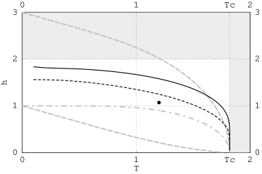
Figure 2: Exact upper bound for the existence of a stable paramagnetic phase on the Bethe lattice of degree $k=2$ (solid line). The bound was obtained as described in the text with all random field configurations at $R=4$. The dashed line is a similar upper bound obtained by considering a sample of $10^{4}$ realizations of the random field at $R=11$ using the complete sum (15). Close to $T=0$ the problem is numerically unstable; results are presented only for $T\geq 0.1$. The large dot was obtained for $R=23$ using (17) and $10^{5}$ random field configurations. In the shaded region the result of brz98 for the existence of a unique paramagnetic phase applies. The grey dashed lines are the ferromagnetic and the antiferromagnetic lines Bruinsma , cf. also brz98 , and the grey dash dotted line is Bruinsma’s lower bound for the existence of a stable ferromagnetic phase Bruinsma . ($J=1$)

To apply the criterion obtained above we evaluated $K$ on a computer. The calculation time is proportional to the number of random field configurations on $V_{R}$ and thus asymptotically grows for, e. g., $k=2$ as $2^{2^{R}}$. Therefore, the calculation was restricted to $R\leq 4$ (for $R=5$ each data point in an array of $20\times 40$ points would take about 3 days on a Pentium II 350MHz). The solid line in Fig. 2 shows the upper bound for the existence of a unique paramagnetic phase obtained for $R=4$.

To estimate the results for $R>4$ we relied on statistical methods and sampled random field configurations. Doing so it is saving time not to exploit the symmetry and use (15) instead of (17). The resulting bound for $R=11$ and a sample of $10^{4}$ random field configurations is the dashed line in Fig. 2.

As the obtained bound systematically depends on the radius $R$ it is tempting to try to extrapolate to $R=\infty$. For $T=1.2$ we obtained an extremely good fit for the data sampled at $R=5$, …, $23$ using $h_{c}(R)=a+bR^{c}$. However, the result was $a=h_{c}(\infty)\approx 0$ which is not realistic. Other fits, e. g. omitting data for small $R$ or using different functional forms, yielded values between $-0.9$ and $0.45$. We suspect that a na$\ddot{\mbox{\i}}$ve choice of the functional form of $h_{c}(R)$ does not allow realistic extrapolation results for these bounds in the case of the Bethe lattice.

IV Estimates for the transition line

IV.1 Direct calculation of the magnetization

Even though the bounds presented in the preceding section considerably improve former analytical results they are still far away from the region where the phase transition from paramagnetic to ferromagnetic behaviour is suspected. In Bruinsma Bruinsma claimed to have found a lower bound in $h$ for the existence of a ferromagnetic phase which is in the relevant parameter region, cf. Fig. 2. To check this bound and to get a good numerical approximation of the transition line we developed several numerical criteria for the existence of a ferromagnetic phase or the existence of a stable paramagnetic phase.

The most obvious criterion for the existence of a ferromagnetic phase is a non-vanishing expectation value for the magnetization for small but non-zero boundary conditions. The expectation value for the local magnetization at the spin in the center is given by

$$m :=\mathbb{E}_{\{\sigma\}}\langle s_{y_{0}}\rangle$$

$$=\int d\nu(x)\,d\nu(y)\,\tanh\big{(}\beta(x+g(y))\big{)}$$ (18)

where $\langle\cdot\rangle$ denotes the thermodynamic average, $\mathbb{E}_{\{\sigma\}}$ the expectation value with respect to all random field configurations and $\nu$ is the limit measure of the effective field for homogeneous boundary conditions $x^{b}_{y}\equiv x^{b}$ for all $y\in V$ in the limit $R\to\infty$. To approximate $\nu$ we generated a large number of random field configurations on a finite region $V_{R}$ and calculated the corresponding effective field $x_{y_{0}}^{\scriptscriptstyle(R)}$. The obtained values were then sorted into small boxes of length $\varepsilon$. The resulting histogram was used as an approximation of $\nu_{y_{0}}(b_{i})=:\nu_{i}$ where $b_{i}$ is the $i$-th box. Explicitly this yields for the magnetization

$$m \approx\sum_{i}\sum_{j}\,\nu_{i}\nu_{j}\,\tanh\beta(x_{i}+g(y_{j})).$$ (19)

where the points $x_{i}$ and $y_{j}$ were chosen as the center of box $i$ and $j$ respectively.

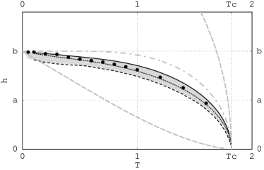
Figure 3: Estimates for the transition line between between para- and ferromagnetism. The dashed line separates regions where the average magnetization decreases or increases with the distance from the boundary for homogeneous boundary conditions $x^{b}\equiv 0.01$ obtained by comparing the configurational averages over $4\cdot 10^{5}$ up to $64\cdot 10^{5}$ samples at distances $9$ and $13$ from the boundary. The dotted line gives the boundary of the region in which the iteration (4) is contractive on the average above and non-contractive below. It was obtained by sampling $10^{5}$ field configurations and evaluating (20) with $R=13$ and $R_{1}=4$. The solid line was obtained using (25) at $R=4$. The big dots were obtained by evaluating (26) for $R=20$ and between $10^{5}$ and $2.4\cdot 10^{6}$ random field configurations. The grey lines are as in Fig. 2. The grey shaded region marks the region all our numerical results (including considerably more than shown explicitly here) are contained in. ($k=2$, $J=1$)

Assuming that the magnetization in the center varies monotonically with the radius $R$ of the finite volume $V_{R}$ one would expect to observe a monotonically increasing magnetization in the ferromagnetic regime and a monotonically decreasing magnetization in the paramagnetic regime for increasing $R$. Therefore, the dashed contour in Fig. 3 which divides the regions in which the numerical estimate of the magnetization is increasing or decreasing with increasing $R$ is a good estimate for the transition line. This type of estimates only slightly depends on the chosen boundary condition and iteration depth but the obtained results significantly disagree with Bruinsma’s bound.

IV.2 Average contractivity of the RIFS

For zero boundary conditions there is a paramagnetic state for any temperature $T$ and random field strength $h$. The stability of this state is tied to the average contractivity of the RIFS (4). If it is globally contracting the paramagnetic state is stable and unique. If it is at least contracting on the average for some interval around zero, the paramagnetic phase is stable but the existence of other stable phases is not a priori excluded. The investigation of the contractivity of the RIFS was first proposed in Heiko .

We generated a set $\Sigma_{R}$ of random field configurations $\{\sigma\}_{R}$ on a finite ball $V_{R}$ and calculated the image of a small initial interval $I^{b}=[-x^{b},x^{b}]$. Because of the monotonicity of $f_{\{\sigma\}_{R}}$ the image of this interval at vertex $y$ is $I_{y}=[x_{y}^{\scriptscriptstyle(R)}(-x^{b}),x_{y}^{\scriptscriptstyle(R)}(x^{b})]$. To estimate the average contractivity of the RIFS we compared the average length $1/k^{R_{1}}\sum_{y\in\partial V_{R_{1}}}|I_{y}|$ at the vertices $y\in\partial V_{R_{1}}$ to the length $|I_{y_{0}}|$ at the central vertex $y_{0}$. As the effective fields at all $y\in\partial V_{R_{1}}$ contribute to the effective field at $y_{0}$ we consider the average interval lengths at vertices in $\partial V_{R_{1}}$ instead of individual values. To minimize the influence of the somewhat arbitrary choice of the initial interval the comparison was performed for $R_{1}\ll R$.

There are two ways of performing the comparison. Either one first averages over the lengths $|I_{y}|$ at all $y\in\partial V_{R_{1}}$ then calculates the quotient of $|I_{y_{0}}|$ and this average length in $\partial V_{R_{1}}$ and average over the sample $\Sigma_{R}$ of random field configurations at the end,

$$\bigg{\langle}\frac{|I_{y_{0}}|}{\frac{1}{k^{R_{1}}}\sum_{y\in\partial V_{R_{1}}}|I_{y}|}\bigg{\rangle}_{\Sigma_{R}}.$$ (20)

Or one first averages $|I_{y}|$ over all $y\in\partial V_{R_{1}}$ and all random field configurations as well as $|I_{y_{0}}|$ over the same random field configurations and calculates the quotient at the end,

$$\frac{\big{\langle}|I_{y_{0}}|\big{\rangle}_{\Sigma_{R}}}{\big{\langle}\frac{1}{k^{R_{1}}}\sum_{y\in\partial V_{R_{1}}}|I_{y}|\big{\rangle}_{\Sigma_{R}}}.$$ (21)

The two averaging procedures (20) and (21) yield identical results and thus obviously are equivalent.

If the images of the initial interval contract on the average for a finite iteration of (4) we expect complete contraction to length zero for infinite iteration. This corresponds to a stable paramagnetic phase. Therefore, the contour in the ($T,h$) parameter plane at which the average quotient of band lengths switches from greater than $1$ below to less than $1$ above is an estimate for the stability region of the paramagnetic phase. The resulting estimated transition line is shown for $R=13$, $R_{1}=4$, the initial interval $I^{b}=[-0.01,0.01]$ and $10^{5}$ random field configurations as the dotted line in Fig. 3. Again, the agreement of the obtained results for various boundary conditions and iteration depths is satisfactory but there is a large deviation from Bruinsma’s line.

IV.3 Independence of the effective fields from boundary conditions

A related criterion for the existence of a stable paramagnetic phase is the independence of the effective field from boundary conditions. As in Sec. III we use the effective fields $g_{y}^{\scriptscriptstyle(R)}$ rather than $x_{y}^{\scriptscriptstyle(R)}$. We consider boundary conditions $\{g^{b}_{y}\}_{y\in\partial V_{R}}$ taking values in a small interval $[-g^{b},g^{b}]$. Through the iteration with (4) the effective fields $g_{y}^{\scriptscriptstyle(R)}$ are functions of the boundary conditions

$$g_{y}^{\scriptscriptstyle(R)}=\tilde{f}_{\{\sigma\}_{R-n-1}(y)}(\{g^{b}_{z}\})$$ (22)

where the function $\tilde{f}_{\{\sigma\}_{R-n-1}(y)}$ has $k^{R-n}$ arguments for $y\in\partial V_{n}$ and it is the identity if $R=n$. For simplicity and without loss of generality we restrict the following discussion to $g_{y_{0}}^{\scriptscriptstyle(R)}$. The boundary conditions can be written as $g^{b}_{y}=g^{b}\,\hat{g}^{b}_{y}$ where $\hat{g}^{b}_{y}$ takes values in $[-1,1]$. To investigate how the effective fields depends on the boundary conditions we consider the expectation value of the derivative of $g_{y_{0}}^{\scriptscriptstyle(R)}$ with respect to $g^{b}$, the strength of the applied boundary condition

$$\mathbb{E}_{\{\sigma\}_{R-1}}\Big{|}\frac{d}{dg^{b}}g_{y_{0}}^{\scriptscriptstyle(R)}\Big{|}$$

$$\hphantom{\mathbb{E}}\leq\mathbb{E}_{\{\sigma\}_{R-1}}\sum_{y\in\partial V_{R}}\partial_{g_{y}}\tilde{f}_{\{\sigma\}_{R-1}}(\{g^{b}_{z}\}_{z\in\partial V_{R}})\,|\hat{g}^{b}_{y}|$$

$$\hphantom{\mathbb{E}}\leq\sum_{y\in\partial V_{R}}\mathbb{E}_{\{\sigma\}_{R-1}}\prod_{l=0}^{R-1}A^{\prime}(x_{z_{l}(y)}^{\scriptscriptstyle(R)}(x^{b}))$$ (23)

where $x_{z_{l}(y)}^{\scriptscriptstyle(R)}(x^{b})$ denotes the effective fields along the unique path from $y$ to $y_{0}$ with homogeneous boundary conditions $x^{b}_{y}\equiv A^{-1}(g^{b})$. Now one can estimate similar as in Appendix A.1

$$A^{\prime}(x_{z_{l}(y)}^{\scriptscriptstyle(R)}(x^{b}))$$

$$\hphantom{A}\leq\min\{A^{\prime}(\max\{x_{z_{l}(y)}^{\scriptscriptstyle(R)}(x^{b}),0\},A^{\prime}(\min\{x_{z_{l}(y)}^{\scriptscriptstyle(R)}(-x^{b}),0\}\}$$

$$\hphantom{A}=:{{A^{\prime}}_{z_{l}(y)}^{\scriptscriptstyle(R)}}_{\mathrm{max}}(x^{b}).$$ (24)

As the boundary conditions are homogeneous this implies

$$\mathbb{E}_{\{\sigma\}_{R-1}}\Big{|}\frac{d}{dg^{b}}g_{y_{0}}^{\scriptscriptstyle(R)}\Big{|}\leq k^{R}\mathbb{E}_{\{\sigma\}_{R-1}}\prod_{l=0}^{R-1}{{A^{\prime}}_{z_{l}(y)}^{\scriptscriptstyle(R)}}_{\mathrm{max}}(x^{b}).$$ (25)

If the right hand side vanishes for $R\to\infty$ the effective field $g_{y_{0}}$ is on the average independent from boundary conditions taking values in $[-g^{b},g^{b}]$. By determining the parameter region in which the right hand side of (25) vanishes for $R\to\infty$ we therefore get an upper bound on the emergence of a stable paramagnetic phase. As our calculations are limited to finite $R$, convergence to zero is assumed if the obtained values of (25) for $R>0$ are smaller than $1$ which is the value for $R=0$.

For the Bethe lattice of degree $k=2$, radius $R=4$ and $g^{b}=0.01$ the right hand side of (25) was evaluated. The contour between values smaller than $1$ above and greater than $1$ below is shown as the solid line in Fig. 3. For $R>4$ we again relied on sampling random field configurations instead. The resulting transition lines for various iteration depths and boundary conditions are comparable to the results of the preceding two sections and are all contained in the grey region in Fig. 3.

If we consider the derivative of the effective field at $y_{0}$ in the case of boundary conditions $g^{b}\equiv 0$ we have

$$\mathbb{E}_{\{\sigma\}_{R-1}}\frac{dg_{y_{0}}^{\scriptscriptstyle(R)}}{dg^{b}}(\{0\}) =\mathbb{E}_{\{\sigma\}_{R-1}}\sum_{y\in\partial V_{R}}\prod_{l=0}^{R-1}A^{\prime}(x_{z_{l}(y)}^{\scriptscriptstyle(R)}(\{0\})).$$ (26)

If this derivative does not tend to zero for some parameters $(T,h)$ and $R\to\infty$ there is no stable paramagnetic phase. By determination of the parameter region in which this is the case we get a lower bound on the emergence of a stable paramagnetic phase. The numerical results are the large dots in Fig. 3.

V Discussion

In order to interpret the discrepancies between Bruinsma’s result and our numerical investigations we briefly review Bruinsma’s argument Bruinsma in our language.

1.  + - + - + - + -     2.  + - - + + - + -
     +   -   +   -           +   -   +   -
       +       -               +       -
           +                       +

3.  + - + - + - + -     4.  + - + - + - + -
     -   +   +   -           +   -   +   -
       +       -               -       +
           +                       +

Figure 4: Four equivalent chessboard configurations at $R=4$. The second configuration is obtained from the first by permutation of two subtrees of a vertex in the sphere $\partial V_{2}$, the third one by permutation of two subtrees of a vertex in the sphere $\partial V_{1}$ and the last one by permutation of the two subtrees of the root itself.

The probability measures $\nu_{y}$ of the effective fields $x_{y}$ are fixed points of the Frobenius-Perron equation, Eq. (7). They can be approximated by finite iterations of some initial probability densities (boundary conditions) $\nu^{b}_{y}$ for $y\in\partial V_{R}$. If the support of $\nu^{b}_{y}$ is a subset of the invariant interval $I$, the support of $\nu_{y_{0}}$ is a subset of the images of $I$ by functions $f_{\{\sigma\}_{R}}$. These images are called bands. The left and right boundary of the bands are the effective fields corresponding to homogeneous boundary conditions $x^{b}_{y}\equiv x^{*}_{+}$ and $x^{b}_{y}\equiv x^{*}_{-}$ for $y\in\partial V_{R}$, respectively. The investigation of the structure of the set of bands has proved to be a powerful tool in the treatment of the one-dimensional random field Ising model gyoergyi1 ; brandtgross ; behn1 ; behn2 ; bene1 ; bene2 ; tanaka1 ; behn5 ; behn6 . In contrast to the one-dimensional case the bands are highly degenerate here, i. e., different configurations of the random field result in the same band. This is due to the invariance of the model with respect to permutations of subtrees for homogeneous boundary conditions. The most degenerate bands correspond to the two chess-board configurations, cf. Fig. 4, of the random field with $+h$ or $-h$ at $y_{0}$ respectively. There are $2^{2^{R-1}-1}$ equivalent random field configurations in the case of the Bethe lattice of degree $k=2$ and radius $R$. As the total number of configurations is $N=2^{2^{R}-1}$ the most degenerate bands have a weight of $2^{2^{R-1}-1}/2^{2^{R}-1}=2^{-2^{R-1}}\sim 1/\sqrt{N}$. The bands with the least weight are the bands corresponding to homogeneous $+h$ or $-h$ random field configurations. They have the weight $1/N$. The weights of all other bands are distributed between these values.

Bruinsma used boundary conditions $\nu^{b}_{y}\equiv\delta_{x^{b}}$ for some $x^{b}\in\mathbb{R}$ and iterated (7). He only considered the lowest and highest weight terms corresponding to the least and the most degenerate bands. The highest weight terms obey a recursion relation. The fixed points of this relation can be calculated and it is straightforward to determine for which temperatures $T$ and random field strengths $h$ they are symmetric to the origin. Proving differentiability of the density $\rho$ of the invariant measure $\nu$ in a neighbourhood of $T=T_{c}$ and $h=0$, Bruinsma concluded that an asymmetric position corresponds to asymmetric maxima of $\rho$ of non-zero weight and therefore to the existence of a ferromagnetic phase.

The symmetric position corresponds to complete contraction of the most degenerate bands such that the asymmetric boundary condition has no effect in the limit of infinite iteration. The asymmetric position on the other hand occurs if the most degenerate bands do not completely contract. Seen this way the argument above is our criterion of average contractivity of the RIFS in Sec. IV.2 except that it is restricted to the contractivity of one specific band instead of the average contractivity.

a) $h=0.3$

b) $h=0.961159$

Figure 5: Approximations of the invariant measure density $\rho$ obtained from four-fold application of (7) to the equipartition $\rho^{b}=|I|^{-1}\cdot{\boldsymbol{1}}_{I}$ on the invariant interval $I$. There are no maxima at $\pm h$ in a) whereas the two maxima at $\pm h$ in b) are already so pronounced that differentiability of $\rho$ is questionable. The random field strength in b) was chosen such that the point $(T,h)$ is very close to Bruinsma’s bound. ($k=2$, $\beta=J=1$)

There are two problematic points in the reasoning above. Firstly, it is not clear whether the location of local maxima in a differentiable measure density really is given by the most degenerate bands. For small $h$ this actually seems not to be the case, cf. Fig. 5a. As the maxima are at $\pm h$ and therefore close to zero for small $h$ it is difficult to argue based on numerical data though. The example in Fig. 5b shows however that the maxima are present for sufficiently large $h$.

Secondly, the differentiability of the invariant measure density has been proved only in a neighbourhood of $T=T_{c}$ and $h=0$ whereas for large $h$ or small $T$, the measure density $\rho$ is clearly not differentiable. It is unclear whether it is differentiable in the region of the lower bound, cf. Fig. 5b.

The disagreement of our numerical work with Bruinsma’s lower bound therefore allows two interpretations. Either Bruinsma’s bound is not true outside the proven region of validity because the most degenerate bands are not a sufficient indicator for the symmetry of $\rho$ when the measure density is not differentiable. Or in the region between our upper bounds for the existence of a stable paramagnetic phase and Bruinsma’s lower bound for the onset of ferromagnetism a stable paramagnetic phase coexists with the — also stable — ferromagnetic phases. This would imply the existence of a first order phase transition and hysteresis loops depending on the strength of the random field in contrast to the hysteresis at $T=0$ shukla which depends on the homogeneous offset of the random field.

In this paper we improved exact upper bounds for the existence of a unique paramagnetic phase in Sec. III which is a further step towards the exact determination of the phase diagram of the RFIM on the Bethe lattice. Furthermore, we presented numerical work leading to various estimates for the actual phase transition line. The direct calculation of the expectation value of the local magnetization in Sec. IV.1, the investigation of the average contractivity of the RIFS (4) at large iteration depths in Sec. IV.2 and the numerical calculation of the derivative of the effective field with respect to the strength of the boundary condition in section IV.3 provided estimates for the stability region of the paramagnetic phase. All results are in good agreement while all disagreeing with the earlier result of Bruinsma Bruinsma . This disagreement motivates further investigations whether the bound for the onset of ferromagnetism given in Bruinsma needs to be reconsidered or whether there really is a coexistence region for stable ferromagnetic and a stable paramagnetic phase.

The work was partially supported by the Cusanuswerk and the DFG (Graduiertenkolleg “Quantenfeldtheorie”).

Appendix A

A.1 Bound on the partial derivatives in (13)

The partial derivatives in (13) are given by

$$\partial_{g_{y}}\tilde{f}_{\{\tilde{\sigma}\}_{R-1}}(\{\delta_{z}\}_{z\in\partial V_{R}}\})$$

$$\hphantom{\partial_{g_{y}}}=\prod_{l=0}^{R-1}A^{\prime}\big{(}f_{\{\tilde{\sigma}\}_{R-1-l}(z_{l}(y))}(\{\varepsilon_{z}\}_{z\in\partial V_{R}})\big{)},$$ (27)

where $\varepsilon_{z}=A^{-1}(\delta_{z})$, $z_{l}(y)\in\partial V_{l}$ are the vertices along the unique path from $y$ to $y_{0}$, cf. also Fig. 1, and $\{\tilde{\sigma}\}_{R-1-l}(z_{l}(y))$ are the signs of the random field configuration on the subtree of depth $R-1-l$ with root $z_{l}(y)$. The terms $f_{\{\tilde{\sigma}\}_{R-1-l}(z_{l}(y))}(\{\varepsilon_{z}\}_{z\in\partial V_{R}})$ are effective fields $x_{z_{l}(y)}^{\scriptscriptstyle(R)}$ corresponding to boundary conditions $\{x_{z}^{b}=\varepsilon_{z}\}_{z\in\partial V_{R}}$. We write $x_{z_{l}(y)}^{\scriptscriptstyle(R)}(\varepsilon)$ for these fields and $x_{z_{l}(y)}^{\scriptscriptstyle(R)}(x^{+})$ and $x_{z_{l}(y)}^{\scriptscriptstyle(R)}(x^{-})$ for the corresponding effective fields with boundary conditions $x_{z}^{b}=x_{z}^{+}$ and $x_{z}^{b}=x_{z}^{-}$ for $z\in\partial V_{R}$. We then can estimate

$$A^{\prime}\big{(}x_{z_{l}(y)}^{\scriptscriptstyle(R)}(\varepsilon)\big{)}$$

$$\hphantom{A^{\prime}}\leq\max\big{\{}A^{\prime}\big{(}x_{z_{l}(y)}^{\scriptscriptstyle(R)}(\varepsilon^{\prime})\big{)}\,\big{|}\,\varepsilon^{\prime}_{z}\in[x_{z}^{-},x_{z}^{+}],z\in\partial V_{R}\big{\}}$$

$$\hphantom{A^{\prime}}=\max\big{\{}A^{\prime}(x)\,\big{|}\,x\in[x_{z_{l}(y)}^{\scriptscriptstyle(R)}(x^{-}),x_{z_{l}(y)}^{\scriptscriptstyle(R)}(x^{+})]\big{\}}$$

$$\hphantom{A^{\prime}}=\min\big{\{}A^{\prime}(\max\{x_{z_{l}(y)}^{\scriptscriptstyle(R)}(x^{-}),0\}),$$

$$\hphantom{\hphantom{A^{\prime}}=\min\big{\{}}A^{\prime}(\min\{x_{z_{l}(y)}^{\scriptscriptstyle(R)}(x^{+}),0\})\big{\}}.$$ (28)

In the last step we used that the maximum of $A^{\prime}$ in an interval $[a,b]$ is at $a$ if $a\geq 0$, at $b$ if $b\leq 0$ and at zero in all other cases. As the effective fields can never be larger than $x^{*}_{+}$ and never smaller than $x^{*}_{-}$ we can for $z\in\partial V_{R}$ estimate $x_{z}^{-}\geq h_{z}+kA(x^{*}_{-})=x_{z}^{\scriptscriptstyle(R+1)}(x^{*}_{-})$ and $x_{z}^{+}\leq h_{z}+kA(x^{*}_{+})=x_{z}^{\scriptscriptstyle(R+1)}(x^{*}_{+})$. This allows to replace $x^{+}$ and $x^{-}$ in the argument of $x_{z_{l}(y)}^{\scriptscriptstyle(R)}$ in (28) and with $x_{z_{l}(y)}^{\scriptscriptstyle(R)}(x_{y}^{\scriptscriptstyle(R+1)}(x^{*}_{\pm}))=x_{z_{l}(y)}^{\scriptscriptstyle(R+1)}(x^{*}_{\pm})$ we get

$$A^{\prime}\big{(}x_{z_{l}(y)}^{\scriptscriptstyle(R)}(\varepsilon)\big{)} \leq\min\big{\{}A^{\prime}(\max\{x_{z_{l}(y)}^{\scriptscriptstyle(R+1)}(x^{*}_{-}),0\}),$$

$$\hphantom{\leq\min\big{\{}}A^{\prime}(\min\{x_{z_{l}(y)}^{\scriptscriptstyle(R+1)}(x^{*}_{+}),0\})\big{\}}$$

$$=:{{A^{\prime}}_{z_{l}(y)}^{\scriptscriptstyle(R)}}_{\mathrm{max}}.$$ (29)

Inserting (29) into (27) then yields

$$\partial_{g_{y}}\tilde{f}_{\{\tilde{\sigma}\}_{R-1}}(\{\delta_{z}\}_{z\in\partial V_{R}}\})\leq\prod_{l=0}^{R-1}{{A^{\prime}}_{z_{l}(y)}^{\scriptscriptstyle(R)}}_{\mathrm{max}}.$$ (30)

A.2 Bounds on the integrals in (14)

Using the independence of the RVs $g_{y}$ of the signs $\{\sigma_{z}\}_{z\in V_{R}\backslash\{y\}}$ and denoting the number of vertices in $V_{R}$ by $|V_{R}|$, i. e., $|V_{R}|=(k^{R+1}-1)/(k-1)$, one obtains

$$\int\limits_{\{\tilde{\sigma}\}_{R}=\{\sigma\}_{R}}\mskip-27.0mud\eta(\{\tilde{\sigma}\})\,(g_{y}^{+}-g_{y}^{-})$$

$$\hphantom{\int\limits_{\{\tilde{\sigma}\}_{R}=\{\sigma\}_{R}}\mskip-27.0mu}=2^{-|V_{R}|+1}\mskip-6.0mu\int\limits_{\tilde{\sigma}_{y}=\sigma_{y}}\mskip-12.0mud\eta(\{\tilde{\sigma}\})\,(g_{y}^{+}-g_{y}^{-})$$

$$\hphantom{\int\limits_{\{\tilde{\sigma}\}_{R}=\{\sigma\}_{R}}\mskip-27.0mu}=2^{-|V_{R}|}\,\mathbb{E}_{\{\sigma\}}(g_{y}^{+}-g_{y}^{-}\,|\,\tilde{\sigma}_{y}=\sigma_{y}).$$ (31)

The function $A$ is antisymmetric which implies $g_{y}^{+}(\{-\sigma\})=-g_{y}^{-}(\{\sigma\})$ and therefore

$$\mathbb{E}(g_{y}^{+}-g_{y}^{-}\,|\,\sigma_{y}=+)=\mathbb{E}(g_{y}^{+}-g_{y}^{-}\,|\,\sigma_{y}=-),$$ (32)

implying

$$\mathbb{E}(g_{y}^{+}-g_{y}^{-})$$

$$\hphantom{\mathbb{E}}=\textstyle\frac{1}{2}\mathbb{E}(g_{y}^{+}-g_{y}^{-}\,|\,\sigma_{y}=+)+\frac{1}{2}\mathbb{E}(g_{y}^{+}-g_{y}^{-}\,|\,\sigma_{y}=-)$$

$$\hphantom{\mathbb{E}}=\mathbb{E}(g_{y}^{+}-g_{y}^{-}\,|\,\sigma_{y}=\sigma),$$ (33)

for any $\sigma\in\{-,+\}$. Setting

$$\mathbb{E}_{R} :=\max_{y\in\partial V_{R}}\mathbb{E}_{\{\sigma\}}(g_{y}^{+}-g_{y}^{-}\,|\,\tilde{\sigma}_{y}=\sigma_{y})$$

$$=\max_{y\in\partial V_{R}}\mathbb{E}_{\{\sigma\}}(g_{y}^{+}-g_{y}^{-}),$$ (34)

this finally yields

$$\int\limits_{\{\tilde{\sigma}\}_{R}=\{\sigma\}_{R}}\mskip-27.0mud\eta(\{\tilde{\sigma}\})\,(g_{y}^{+}-g_{y}^{-})\leq 2^{-|V_{R}|}\,\mathbb{E}_{R}.$$ (35)

References

- (1) T. Nattermann, in Spin glasses and random fields, edited by A. P. Young (World Scientific, Singapore, 1998), p. 277, and references therein.
- (2) D. P. Belanger, in Spin glasses and random fields, edited by A. P. Young (World Scientific, Singapore, 1998), p. 251, and references therein.
- (3) P. M. Bleher, J. Ruiz, and V. A. Zagrebnov, J. Stat. Phys. 93, 33 (1998).
- (4) R. Bruinsma, Phys. Rev. B 30, 289 (1984).
- (5) R. Bruinsma and G. Aeppli, Phys. Rev. Lett. 50, 1494 (1983).
- (6) G. Aeppli and R. Bruinsma, Phys. Lett. 97A, 117 (1983).
- (7) P. Ruján, Physica A 91, 549 (1978).
- (8) G. Györgyi and P. Rujàn, J. Phys. C 17, 4207 (1984).
- (9) U. Brandt and W. Gross, Z. Phys. B 31, 237 (1978).
- (10) P. Szépfalusy and U. Behn, Z. Phys. B 65, 337 (1987).
- (11) U. Behn and V. A. Zagrebnov, JINR, E 17-87-138 Dubna (1987); J. Stat. Phys. 47, 939 (1987); J. Phys. A 21, 2151 (1988); Phys. Rev. B 38, 7115 (1988).
- (12) J. Bene and P. Szépfalusy, Phys. Rev. A 37, 1703 (1988).
- (13) J. Bene, Phys. Rev. A 39, 2090 (1989).
- (14) T. Tanaka, H. Fujisaka, and M. Inoue, Phys. Rev. A 39, 3170 (1989); Prog. Theor. Phys. 84, 584 (1990).
- (15) U. Behn, V. B. Priezzhev and V. A. Zagrebnov, Physica A 167, 481 (1990).
- (16) U. Behn and A. Lange, in From Phase Transitions to Chaos, edited by G. Györgyi, I. Kondor, L. Sasvári and T. Tél (World Scientific, Singapore, 1992) p. 217.
- (17) H. Patzlaff, Dissertation, Universität Leipzig (1997).
- (18) M. R. Swift, A. Maritan, M. Cieplak and J. R. Banavar, J. Phys. A 27, 1525 (1994).
- (19) U. Brandt, J. Magn. Magn. Mater. 15, 223 (1980).
- (20) H. O. Georgii, Gibbs Measures and Phase Transitions (Walter de Gruyter, New York, 1988).
- (21) D. Dhar, P. Shukla, and J. P. Sethna, J. Phys. A 30, 5259 (1997); S. Sabhapandit, P. Shukla, and D. Dhar, J. Stat. Phys. 98, 103 (2000); P. Shukla, Phys. Rev. E 62, 4725 (2000); Phys. Rev. E 63, 027102 (2001).