Plaquette-singlet solid state and topological hidden order
in spin-1 antiferromagnetic Heisenberg ladder

Abstract

Ground-state properties of the spin-1 two-leg antiferromagnetic ladder are investigated precisely by means of the quantum Monte Carlo method. It is found that the correlation length along the chains and the spin gap both remain finite regardless of the strength of interchain coupling, i.e., the Haldane state and the spin-1 dimer state are connected smoothly without any quantum phase transitions between them. We propose a plaquette-singlet solid state, which qualitatively describes the ground state of the spin-1 ladder quite well, and also a corresponding topological hidden order parameter. It is shown numerically that the new hidden order parameter remains finite up to the dimer limit, though the conventional string order defined on each chain vanishes immediately when infinitesimal interchain coupling is introduced.

]

I Introduction

Quantum spin-ladder systems have been studied theoretically and experimentally over the last decade as materials with a novel spin-gap state, as well as by their relevance to the high-temperature superconductivity. [5] Especially, the two-leg ladder Heisenberg antiferromagnet, which is defined by the Hamiltonian:

$${\cal H} = J\sum_{i}\left\{{\bf S}_{1,i}\cdot{\bf S}_{1,i+1}+{\bf S}_{2,i}\cdot{\bf S}_{2,i+1}\right\}$$ (2)

$$+K\sum_{i}{\bf S}_{1,i}\cdot{\bf S}_{2,i},$$

has been studied most extensively. Here, ${\bf S}_{\alpha,i}$ is the spin operator at site $i$ on the $\alpha$-th chain ($\alpha=1,2$), and the intrachain and interchain coupling constants are denoted by $J$ and $K$, respectively. In the following, we restrict our attention only to the case in which the intrachain coupling is antiferromagnetic ($J>0$). On the other hand, the interchain coupling constant, $K$, can be either positive (antiferromagnetic) or negative (ferromagnetic).

At $K=0$, the system consists of two decoupled antiferromagnetic Heisenberg chains. In this case, it is well known that the ground-state properties can be classified into two universality classes depending on the parity of $2S$. Here $S$ is the spin size. In the case where $S$ is a half-odd integer, the ground state is critical, i.e., the system has gapless low-lying excitation and the antiferromagnetic correlation function along the chain decays in an algebraic way as the distance increases. On the other hand, it is conjectured by Haldane[6] that the antiferromagnetic Heisenberg chain of integer spins has a finite excitation gap above its unique ground state, and the correlation function decays exponentially with a finite correlation length. Its ground-state properties can be understood quite well from the viewpoint of the valence-bond solid (VBS) picture,[7] in which the ground state is essentially represented as direct products of spin-$\frac{1}{2}$ dimers (AKLT state). In addition, a topological order parameter characterizing the AKLT state, as well as the Haldane state, so-called the string order parameter, has been proposed.[8] The validity of Haldane’s conjecture has been confirmed precisely for $S=1$, 2, and 3 by several numerical methods.[9, 10, 11, 12, 13]

Introduction of non-zero interchain coupling, $K$, is known to drastically change the ground state, at least for the spin-$\frac{1}{2}$ case.[5] For small $K$, either antiferromagnetic or ferromagnetic, it immediately opens a spin gap of $O(|K|)$ with some logarithmic corrections. [14] That is, $K=0$ is the special point at which there occurs a quantum second-order phase transition between the dimer phase ($K>0$) and the spin-1 Haldane phase ($K<0$). Again, from the viewpoint of VBS picture, one can understand this phase transition as a global rearrangement of dimer pattern. For larger half-odd-integer spins ($S=\frac{3}{2}$, $\frac{5}{2}$, $\cdots$), the criticality at $K=0$ should be essentially the same as in the spin-$\frac{1}{2}$ case.

In the case of integer-spin chains, on the other hand, effects of interchain coupling have been known little so far. Recently, Sénéchal and Allen studied the spin-1 ladder by mapping it to the nonlinear $\sigma$ model[15] and also by the bosonization technique.[16] They found that in contrast to the spin-$\frac{1}{2}$ case, small interchain coupling reduces the magnitude of the spin gap in both of antiferromagnetic and ferromagnetic regimes. In addition, their analyses as well as their complemental Monte Carlo calculation suggest that there is no critical point between the Haldane and the spin-1 dimer phases. This may seem paradoxical since these two phases have apparently different dimer patterns from each other.

In this paper, we present the results of our extensive quantum Monte Carlo simulation on the spin-1 ladder. After reviewing details of our simulation using the efficient continuous-time loop algorithm in Sec. II, we present our numerical data on the uniform susceptibility, staggered susceptibility, antiferromagnetic correlation length, etc. in Sec. III, which convincingly demonstrate the continuity of the two limiting case ($K=0$ and $K=\infty$), and thus support the conjecture by the previous analytical approaches.[15, 16] In Sec. IV, we propose a plaquette-singlet solid state, which is constructed as products of local singlet states of four $S=\frac{1}{2}$ spins. The Haldane state and the spin-1 dimer state are naturally included as special limits. In addition, we propose a kind of hidden order parameter, which can detect the topological hidden order exsisting in the plaquette-singlet solid state. We show numerically that the new hidden order parameter we propose remains finite in the whole parameter range, $0\leq K\leq\infty$, while the conventional string order parameter vanishes except at $K=0$. In Sec. V, we consider in turn the case where the interchain coupling is ferromagnetic ($K<0$), and show that the spin-1 Haldane state and that of $S=2$ also continue to each other without any singularity on the way to the other. We give a summary of our results and some discussions in the final section.

II Quantum Monte Carlo Method

A Continuous-time loop algorithm for spin-1 system

The recently-developed continuous-time loop algorithm [17, 18, 19] is one of the most efficient methods for simulating quantum spin systems. It is a variant of the world-line Monte Carlo method, which is based on the path-integral representation by means of the Suzuki-Trotter discretization. [20] However, the continuous-time loop algorithm works directly in the imaginary-time continuum, [19] and thus is completely free from the systematic error in the Suzuki-Trotter discretization. In addition, the correlation between successive spin configurations is greatly reduced, sometimes by orders of magnutide, since it flips effectively clusters of spins, or loops, whose linear sizes correspond directly to the length scale of relevant spin fluctuations. The algorithm has already been applied to various spin systems with great success. [21]

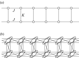
FIG. 1.: (a) Original spin-1 ladder, and (b) equivalent system represented by $S=\frac{1}{2}$ spins (subspins). The spin-1 ladder of length $L$ ($2L$ spins and $3L$ bonds) is mapped onto the spin-$\frac{1}{2}$ system on a lattice of $4L$ subspins and $12L$ bonds. Each oval in (b) denotes a pair of subspins which is symmetrized by being applied special boundary conditions in the imaginary-time direction.

The Hamiltonian we consider is given by Eq. (2) with $S=1$. The linear size along the chain is denoted by $L$, and we adopt periodic boundary conditions in this direction, i.e., ${\bf S}_{\alpha,i+L}={\bf S}_{\alpha,i}$ for $\alpha=1$ and 2. In order to apply the continuous-time loop algorithm to the present spin-1 system, first we represent the spin-1 Hamiltonian in terms of subspins. In this representation, each spin-1 operator in Eq. (2) is decomposed into a sum of two spin-$\frac{1}{2}$ operators. [22] Simultaneously, each bond of strength $J$ (or $K$) is transformed into four bonds of the same strength connecting subspins. The lattices before and after the subspin transformation are shown in Fig. 1. Note that in order to recover dimensions of the original spin-1 Hilbert space ($3^{2L}$), one needs to introduce a set of projection operators, each of which acts on a pair of subspins and projects out the state with $S=0$ (Fig. 1). After transformed into a path-integral representation, the projection operators are converted to special boundary conditions in the imaginary-time direction; [13, 23] for each pair of subspins, the total $S^{z}$ is required to be conserved across the imaginary-time boundary.

For the mapped system, the spin-$\frac{1}{2}$ continuous-time loop algorithm [17, 18, 19] can be applied without any modification except that we need to introduce additional graphs and labeling rules for the boundaries in the imaginary-time direction. [13, 23] We use the multi-cluster variant of the loop algorithm. The resulting algorithm is found to work quite well as the same as the original algorithm developed for $S=\frac{1}{2}$; the integrated auto-correlation time for the physical quantities we measure remains of order unity, and there is observed no significant sign of its growth even in the largest system in the present simulation ($L=1024$ and $T/(J+K)=2/1024\simeq 0.00195$).

B Physical quantities

The physical quantities of interest can be measured by using the corresponding subspin representations. First, for later convenience, we introduce the imaginary-time dynamical correlation function, $C^{\pm}(x,\tau)$, and its Fourier transform, ${\tilde{C}}^{\pm}(k,\omega)$. The former is defined explicitly in the path-integral representation by

$$C^{\pm}(x,\tau) = \frac{1}{2L\beta}\Big{<}\int_{0}^{\beta}\!\!\!\!dt\sum_{i}\left\{{\cal S}_{1,i}(t)\pm{\cal S}_{2,i}(t)\right\}$$ (4)

$$\quad\times\left\{{\cal S}_{1,i+x}(t+\tau)\pm{\cal S}_{2,i+x}(t+\tau)\right\}\Big{>}\,,$$

where $\beta$ is the inverse temperature ($=1/T$). The spin configuration at site $i$ on the $\alpha$-th chain and at imaginary time $\tau$ $(0\leq\tau\leq\beta)$ is denoted by ${\cal S}_{\alpha,i}(\tau)$, which takes -1, 0, or 1. The bracket $\left<\cdots\right>$ in Eq. (4) denote the average over Monte Carlo steps (MCS). In the present subspin representation, ${\cal S}_{\alpha,i}(\tau)$ is simply given by a sum of $S^{z}$ of two subspins at $(\alpha,i,\tau)$.

In terms of the imaginary-time dynamic structure factor, $\tilde{C}^{\pm}(k,\omega)$, the uniform susceptibility and the staggered susceptibility are simply given by

$$\chi=2L\beta\tilde{C}^{+}(0,0)$$ (5)

and

$$\chi_{\rm s}=2L\beta\tilde{C}^{-}(\pi,0),$$ (6)

respectively. We also calculate the static structure factor at momentum $\pi$ as

$$S(\pi) = \frac{1}{2L}\Big{<}\sum_{i,j}(-1)^{|i-j|}\big{(}{\cal S}_{1,i}(0)-{\cal S}_{2,i}(0)\big{)}$$ (8)

$$\quad\quad\times\big{(}{\cal S}_{1,j}(0)-{\cal S}_{2,j}(0)\big{)}\Big{>}.$$

In order to calculate the correlation length along the chains, we use the second-moment method: [24]

$$\xi=\frac{L}{2\pi}\sqrt{\frac{\tilde{C}^{\pm}(\pi,0)}{\tilde{C}^{\pm}(\pi+2\pi/L,0)}-1}.$$ (9)

Similarly, the spin gap, which is defined as the inverse of the correlation length in the imaginary-time direction, is measured by

$$\Delta^{-1}=\frac{\beta}{2\pi}\sqrt{\frac{\tilde{C}^{\pm}(\pi,0)}{\tilde{C}^{\pm}(\pi,2\pi/\beta)}-1}.$$ (10)

In Eqs. (9) and (10), we take the minus (plus) sign for $K>0$ ($K<0$). Although the above second-moment estimates suffer from systematic error due to the existence of subdominant decaying modes in the correlation function, it should be sufficiently small (at $K=0$ the systematic error for the spin gap is known to be about 0.2% [13]), and thus we expect that it would be irrelevant to the following discussions. We will also present our results for the string order parameter [8] and a new hidden order parameter in Sec. IV. Their explicit definitions will be given later.

TABLE I.: Convergence of physical quantities at $J=0.7$ and $K=0.3$. The temperature is taken as $T/(J+K)=2/L$ for each $L$. The figure in parentheses denotes the statistical error ($2\sigma$) in the last digit. There are observed no significant differences between the data with $L=256$, 512, and 1024.

$L$	MCS	$(J+K)\,\chi_{\rm s}$	$S(\pi)$	$\Delta/(J+K)$	$\xi$
8	$3\times 10^{5}$	16.48(3)	4.95(1)	0.3863(6)	4.57(1)
16	$6\times 10^{5}$	49.72(8)	7.74(1)	0.2120(3)	8.50(1)
32	$7\times 10^{5}$	138.0(2)	11.39(2)	0.1218(2)	14.86(2)
64	$1\times 10^{6}$	315.9(4)	14.97(2)	0.0793(1)	22.81(3)
128	$1\times 10^{6}$	468.7(8)	16.23(2)	0.06602(9)	27.37(4)
256	$7\times 10^{5}$	489.8(5)	16.19(2)	0.06487(7)	27.91(4)
512	$3\times 10^{5}$	490.3(3)	16.17(2)	0.06477(8)	27.93(3)
1024	$2\times 10^{5}$	490.1(2)	16.17(2)	0.06476(4)	27.92(2)

In practice, all the physical quantities we will show in the following, including the hidden order parameters, are measured by using so-called improved estimators. For example, the staggered susceptibility for $K>0$ is simply represented as the sum of squared length of each loop, divided by $8L\beta$. Similarly, the imaginary-time dynamic structure factor can be measured directly as

$${\tilde{C}}^{\pm}(k,\omega)=\frac{1}{4L^{2}\beta^{2}}\left<\sum_{p}\left|\frac{1}{2}\oint(\pm 1)^{\alpha}e^{i(kx+\omega t)}d\ell\right|^{2}\right>,$$ (11)

where the integration is performed along a closed path on each loop, and the summation runs over all loops.

C Taking the thermodynamic limit and the zero-temperature limit

In the present method, the system size, $L$, and the temperature, $T$, are restricted to be finite. [25] Since we are mainly interested in the ground-state properties of the infinite lattice, a proper extrapolation scheme for taking the thermodynamic limit ($L\rightarrow\infty$) as well as the zero-temperature one ($T\rightarrow 0$) is required. In the present study, we adopt the following strategy, which is the same as was used in Ref. [13] for the estimation of the Haldane gap of the antiferromagnetic Heisenberg chain with $S=1$, 2, and 3.

For each parameter set $(J,K)$, we start with a small lattice at relatively high temperature, e.g., $L=8$ and $T/(J+K)=0.25$. Then, we increase the system size exponentially step by step, like $L=16$, 32, 64, 128, $\cdots$. Simultaneously, the temperature is decreased so as to keep $LT/(J+K)=L/(J+K)\beta$ constant. In other words, the aspect ratio of the (1+1)-dimensional space is kept unchanged for all $L$’s. If the system is gapless, the finite-size scaling holds; the correlation length in the real-space direction, $\xi(L,T)$, and that in the imaginary-time direction, $\Delta^{-1}(L,T)$, both would grow being proportional to $L$. [26] Simultaneously, the other physical quantities, such as the staggered susceptibility, should exhibit power-law behavior with some exponents depending on their own anomalous dimensions.

On the other hand, if the system is gapful (this is the case for the present system as we will see below), there exist finite intrinsic correlation lengths, $\xi$ and $\Delta^{-1}$. As long as the system size and the inverse temperature are smaller enough than these intrinsic correlation lengths, the critical behavior above mentioned is still observed. However, once both of $L$ and $\beta$ exceed them enough, $\xi(L,T)$ and $\Delta(L,T)$, as well as other physical quantities, no longer exhibit system-size dependence. Strictly speaking, the systematic error due to the finiteness of the system decreases exponentially as the system size increases, and it becomes much smaller than the statistical error due to the finiteness of MCS.

In Table I, we show the system-size (and temperature) dependence of the physical quantities at $(J,K)=(0.7,0.3)$. As seen clearly, the data with $L\geq 256$ (and with $T/(J+K)\leq 2/256=0.0078125$) exhibit no system-size dependence. Thus, in this case, one can safely conclude that the system is gapful and also that the physical quantities obtained are those of the infinite lattice at zero temperature besides the statistical error. Empirically, we find that $L/\xi(L,T)>6$ with $\beta\Delta(L,T)>6$ is a reasonable condition to guarantee the convergence in the present numerical accuracy.

One of the advantages of the present scheme is that it depends on no numerical extrapolation techniques, such as least-squares fitting, the Shanks transform, etc. Final results are simply obtained from those of the largest system at the lowest temperature in the simulation. Therefore, this method is quite stable and the error estimation is also quite reliable. It should be emphasized that the final results are not affected at all by the value chosen for the aspect ratio, $L/(J+K)\beta$ (=2 in the present case). However, if one chooses a too small or too large value, the physical memory of the computer system might be exhausted before reaching the thermodynamic limit or the zero-temperature one.

In what follows, we will mainly present the data with $L=256$ and $T/(J+K)=2/256$ unless otherwise noted. Measurement of physical quantities is performed for $5\times 10^{5}\sim 1\times 10^{6}$ MCS after $10^{3}$ MCS for thermalization. Typically, simulation of this system requires about 7MB of physical memory, and 1 MCS takes about 0.33 sec. on a single CPU of SGI 2800 (MIPS R12000 400MHz). This system size is somewhat exaggerated for certain sets of parameters, $(J,K)$. However, in such cases, the system can be considered as ${\cal N}$ statistically-independent samples simulated in parallel, where ${\cal N}\sim(L/\xi)\times(\Delta\beta)$. Therefore, we gain better statistics proportional to $\sqrt{\cal N}$, which completely compensates for the growth of CPU time ($\sim L\beta$ for large $L$ and $\beta$). [27] Thus, we loose nothing besides the memory requirement. This is already manifested in the figures presented in Table I.

III Numerical Results

A Parameterization

The ground state of the present system is parametrized by the ratio of the interchain coupling constant to the intrachain one, $x\equiv K/J$. Hereafter, we mainly use $R$, which is defined by

$$R=\frac{K}{J+|K|}=\frac{x}{1+|x|}\,.$$ (12)

Since we consider only the antiferromagnetic intrachain coupling ($J\geq 0$), $-1\leq R\leq 1$. At $R=0$, the system consists of two independent antiferromagnetic chains (spin-1 Haldane chains). On the other hand, at $R=1$, it is decoupled into dimers sitting on each rung. The limit $R\rightarrow-1$ corresponds to a single spin-2 antiferromagnetic chain. We also introduce the reduced temperature, $\tilde{T}=T/(J+K)$, reduced susceptibilities, $\tilde{\chi}=(J+K)\chi$ and $\tilde{\chi_{\rm s}}=(J+K)\chi_{\rm s}$, and the reduced gap, $\tilde{\Delta}=\Delta/(J+K)$. In this section and Sec. IV, we consider only the case where $0\leq R\leq 1$, i.e., the interchain coupling is antiferromagnetic.

B Uniform susceptibility

FIG. 2.: Temperature dependence of the uniform susceptibility for $R=0$ (squares), 0.2 (circles), 0.3 (upward triangles), 0.4 (diamonds), 0.6 (downward triangles), and 0.8 (pentagons). The exact result for $R=1$ (Eq. (13)) is plotted by a solid line. In the inset, the same data are plotted against the logarithm of $\tilde{T}$.

Before investigating the zero-temperature properties of the spin-1 ladder, first we briefly discuss finite-temperature behavior of the uniform susceptibility, which gives a rough profile on the excitation spectrum of the system. In Fig. 2, $\tilde{\chi}$ is plotted as a function of $\tilde{T}$ for $R=0$, 0.2, 0.3, 0.4, 0.6, 0.8, and 1. At $R=1$, i.e., $J=0$, since the system consists of independent dimers, the exact form of the uniform susceptibility is easily obtained as

$$\tilde{\chi} = \frac{1}{\tilde{T}}\,\frac{\exp(-1/\tilde{T})+5\exp(-3/\tilde{T})}{1+3\exp(-1/\tilde{T})+5\exp(-3/\tilde{T})}$$ (13)

$$\simeq \frac{1}{\tilde{T}}\,\exp(-1/\tilde{T})\,\,\,\,\,\,\mbox{for $\tilde{T}\ll 1$.}$$ (14)

At $R=0$, $\tilde{\chi}$ is also known to vanish at low temperatures exponentially as $\exp(-\tilde{\Delta}/\tilde{T})$ with $\tilde{\Delta}\simeq 0.41050(2)$ [10] besides a prefactor of some powers of $T$. As seen clearly in Fig. 2, the temperature dependence of the uniform susceptibility does not depend on the value of $R$ strongly; it has a very broad peak around $\tilde{T}\simeq 1$, and decreases quite rapidly at lower temperatures. It suggests spin-singlet ground state regardless of the value of $R$.

However, it should be noted that at temperatures lower than $\tilde{T}\simeq 0.4$, the uniform susceptibility is not a monotonic function of $R$. It is greatly enhanced by orders of magnitude around $R=0.3$, in comparison with those at $R=0$ and 1. It indicates that in the intermediate region of $R$, the spin gap is strongly suppressed, and on the other hand long-range antiferromagnetic fluctuations are enhanced, due to the competition between the intrachain and the interchain antiferromagnetic couplings.

In addition, in the temperature profile of the uniform susceptibility for $0.2\leq R\leq 0.6$, one can see a clear shoulder structure at $\tilde{T}\simeq 0.1$ (see also the inset of Fig. 2), which indicates existence of some additional anomalies in the excitation spectrum of the system.

FIG. 3.: $R$-dependence of the staggered susceptibility (open squares) and the static structure factor at momentum $\pi$ (solid circles). The statistical error of each data point is much smaller than the symbol sizes.

C Quantities at zero temperature

The temperature dependences of the staggered susceptibility, $\tilde{\chi}_{\rm s}$, and the static structure factor, $S(\pi)$, are found to be qualitatively very similar to those of the single Haldane chain ($R=0$); they grow rapidly around $\tilde{T}\simeq 1$ and are saturated to finite values at low temperatures, though the saturation temperature strongly depends on $R$ (see the $R$-dependence of $\Delta$ shown below). As for $S(\pi)$, in addition, it makes a weak peak before saturated to the zero-temperature value, which indicates a short-range antiferromagnetic order.

In Fig. 3, the zero-temperature values of $\tilde{\chi}_{\rm s}$ and $S(\pi)$ are plotted as a function of $R$. The value of $\tilde{\chi}_{\rm s}$ at $R=0$ is consistent with that obtained in the previous work, $\tilde{\chi}_{\rm s}=18.4048(7)$ [13]. On the other hand, at $R=1$, they coincide the exact values, $\tilde{\chi}_{\rm s}=\frac{8}{3}$ and $S(\pi)=\frac{4}{3}$, respectively, within the statistical error. One sees in Fig. 3 that they are smooth functions of $R$, and thus there is no indication of singularities in the whole range of $R$.

FIG. 4.: $R$-dependence of the inverse correlation length along the chains (solid circles) and the spin gap (open squares). The statistical error of each data point is much smaller than the symbol sizes.

The non-existence of phase transitions is also confirmed by the $R$-dependence of the spin gap, $\tilde{\Delta}$, and the inverse correlation length, $\xi^{-1}$ (Fig. 4). These results convincingly support the conjecture made in the previous analytic studies. [15, 16] It should be recalled that by using the method we explained in detail in Sec. II C, the convergence to the thermodynamic and the zero-temperature limits of the data has been checked for all the value of $R$ we simulated. Therefore, the data can be identified with those at $L=\infty$ and $T=0$ besides the statistical errors, which are much smaller than the symbol sizes in Figs. 3 and 4.

Although there are no singularities between $R=0$ and 1, long-range antiferromagnetic fluctuations are greatly enhanced in the intermediate region of $R$. This is consistent with the temperature dependence of the uniform susceptibility presented in Sec. III B. Especially, note that all the physical quantities we calculated have its maximum (or minimum) at $R\simeq 0.3$ (see also Table I). They could be compared with those of the spin-2 antiferromagnetic Heisenberg chain, i.e., $\tilde{\chi}_{\rm s}=1164.0(2)$, $\xi=49.49(1)$, and $\tilde{\Delta}=0.08917(4)$. [13]

IV Plaquette-Singlet Solid State and Hidden Order Parameter

A Breakdown of AKLT picture

As we have already mentioned in Sec. I, the ground state of the spin-1 antiferromagnetic chain is understood quite well by means of the VBS picture. [7] Actually, the AKLT state, which is the exact ground state of the so-called AKLT model, [7] shares many common properties, such as spin-rotation symmetry, finite correlation length, etc., with the ground state of the spin-1 Heisenberg chain. These two states are believed to belong to the same universality class with each other.

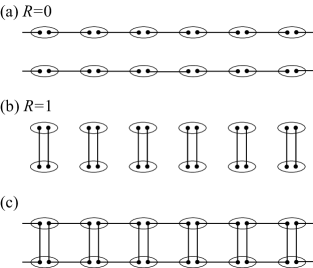
FIG. 5.: Schematic picture of plaquette-singlet solid state. (a) AKLT state at $R=0$. (b) Spin-1 dimer state at $R=1$ (c) Plaquette-singlet solid state for $0<R<1$.

The AKLT state is essentially constructed as direct products of spin-$\frac{1}{2}$ dimers sitting on each bond (Fig. 5(a)). On each site, two edge $S=\frac{1}{2}$ spins are symmetrized to form an $S=1$ spin. An important feature of this state is that a sum of $S^{z}$ in any interval $[i,j]$ can take only 1, 0, or -1. This fact is immediately followed by the existence of a topological hidden order; if one removes spins at $S^{z}=0$ state, the sequence of $S^{z}$ of the remaining spins has a perfect antiferromagnetic-like ordering (1, -1, 1, -1, $\cdots$), although the original one has no ‘true’ antiferromagnetic long-range order at all.

The above topological order in the AKLT state can be detected quantitatively by means of the string order parameter,[8] which is defined by

$$\langle{\cal O}_{2}\rangle=\lim_{|i-j|\rightarrow\infty}\langle{\cal O}_{2}(i,j)\rangle$$ (15)

in terms of the string correlation operator:

$${\cal O}_{2}(i,j)=-S_{i}^{z}\exp\left[i\pi\sum_{k=i+1}^{j-1}S_{k}^{z}\right]S_{j}^{z}\,,$$ (16)

whose expected value is $\frac{4}{9}=0.444\cdots$ for any $|i-j|>1$. The string order parameter (15) is also finite in the spin-1 Heisenberg chain. Its value is estimated to be 0.3743(1) in the thermodynamic limit ($R=0$ in Fig. 6). In practice, the string order parameter of a finite chain of length $L$ is calculated as

$$\langle{\cal O}_{2}\rangle_{L}=\frac{1}{L}\sum_{i}\langle{\cal O}_{2}(i,i+L/2)\rangle\,.$$ (17)

Although the string correlation function (16) is a non-local quantity, one can construct an improved estimator even for it. For details, see Ref. [28].

In the presence of the interchain coupling, however, the above AKLT picture breaks down immediately. As shown in Fig. 6, the string order parameter, $\langle{\cal O}_{2}\rangle_{L}$, defined on one of the two chains, decreases quite rapidly as $R$ increases. Furthermore, in contrast to the other quantities shown before, the value of $\langle{\cal O}_{2}\rangle_{L}$ exhibits strong system-size dependence for $R>0$. Actually, as shown in the inset of Fig. 6, one finds that these finite-size data scale exponentially quite well as

$$\langle{\cal O}_{2}\rangle_{L}\simeq\tilde{f}(R\,\log^{\alpha}\!L)$$ (18)

with $\alpha=2.5$, where $\tilde{f}(x)$ is a scaling function, and it vanishes for $x\rightarrow\infty$. This strongly suggests that the string order parameter (15) is essentially singular at $R=0$, and is vanished by infinitesimal interchain coupling, though we have no account for the value of the exponent $\alpha$ at the moment.

B Plaquette-singlet solid state

As we have seen above, the AKLT picture (Fig. 5 (a)) breaks down immediately for $R>0$. Actually, in the $R=1$ limit, the ground state is represented schematically by a pattern of spin-$\frac{1}{2}$ dimers, in which two dimers are sitting on each rung (Fig. 5 (b)). There is no overlap between these two VBS states.

However, if we focus our attention on a plaquette containing four spins at $(\alpha,x)=(1,i)$, $(1,i+1)$, $(2,i)$, and $(2,i+1)$, it is found that these two states share a remarkable feature, i.e., the sum of $S^{z}$ of these four spins can take only 0, $\pm 1$, or $\pm 2$, and its absolute value never exceeds 2 in both cases. In other words, four $S=\frac{1}{2}$ spins, each of which belongs to an $S=1$ spin at one of four corners of a plaquette, form an $S=0$ state, though its fine structure is quite different from each other. This observation leads us to a proposal of the following generalized state, which connects these two VBS states smoothly.

First, we define a local state of plaquette consisting of four $S=\frac{1}{2}$ spins, which is expressed explicitly as

$$|\psi(\theta)\rangle_{i} = a_{\theta}\Big{[}\cos\theta\left\{|\!\uparrow\rangle_{1,i}|\!\downarrow\rangle_{1,i+1}-|\!\downarrow\rangle_{1,i}|\!\uparrow\rangle_{1,i+1}\right\}$$ (22)

$$\quad\times\left\{|\!\uparrow\rangle_{2,i}|\!\downarrow\rangle_{2,i+1}-|\!\downarrow\rangle_{2,i}|\!\uparrow\rangle_{2,i+1}\right\}$$

$$\quad+\sin\theta\left\{|\!\uparrow\rangle_{1,i}|\!\downarrow\rangle_{2,i}-|\!\downarrow\rangle_{1,i}|\!\uparrow\rangle_{2,i}\right\}$$

$$\quad\times\left\{|\!\uparrow\rangle_{1,i+1}|\!\downarrow\rangle_{2,i+1}-|\!\downarrow\rangle_{1,i+1}|\!\uparrow\rangle_{2,i+1}\right\}\Big{]}\,,$$

where $a_{\theta}$ is the overall normalization factor ($a_{\theta}^{-1}=\sqrt{4+2\sin 2\theta}$). This state is constructed as a superposition of two $S=0$ states. The first term of r.h.s. in Eq. (22) is the product of the dimers sitting on legs, and the second one does that of the rung dimers. The parameter $\theta$ ($0\leq\theta\leq\frac{\pi}{2}$) controls the proportion of these two constituents. Note that the wave function (22) is the exact ground state of the following four-body spin-$\frac{1}{2}$ Hamiltonian:

$${\cal H}_{\rm p} = \frac{J_{\rm p}}{4}(\sigma_{1,i}\cdot\sigma_{1,i+1}+\sigma_{2,i}\cdot\sigma_{2,i+1})$$ (24)

$$\,\,\,\,\mbox{}+\frac{K_{\rm p}}{4}(\sigma_{1,i}\cdot\sigma_{2,i}+\sigma_{1,i+1}\cdot\sigma_{2,i+1})\,,$$

where $J_{\rm p}\geq 0$, $K_{\rm p}>0$, and $\sigma_{\alpha,i}$ denotes the spin-$\frac{1}{2}$ Pauli operator. In this case, the parameter $\theta$ in Eq. (22) can be expressed explicitly as a function of $x_{\rm p}\equiv K_{\rm p}/J_{\rm p}$ as

$$\theta=\arctan\left(x_{\rm p}-1+\sqrt{1-x_{\rm p}+x_{\rm p}^{2}}\right)\,,$$ (25)

and the gap above the ground state never closes throughout while one varies $x_{\rm p}$ from 0 ($\theta=0$) to $\infty$ ($\theta=\frac{\pi}{2}$), as we will see in Sec. VI.

FIG. 6.: $R$-dependence of the hidden order parameters, $\langle O_{2}\rangle$ (open symbols) and $\sqrt{\langle O_{4}\rangle}$ (solid circles). The statistical error of each data point is much smaller than the symbol sizes. The horizontal dashed line denotes the exact value ($\frac{2}{3}$) of $\sqrt{\langle O_{4}\rangle}$ in the dimer limit ($R=1$). A scaling plot for $\langle O_{2}\rangle$ with exponent $\alpha=2.5$ is also shown in the inset.

By using the local singlet state (22), we construct a wave function of the spin-1 ladder:

$$|\Psi(\theta)\rangle_{\rm ps}=\prod_{\alpha,i}{\cal P}_{\alpha,i}\prod_{i}|\psi(\theta)\rangle_{i}\,,$$ (26)

where ${\cal P}_{\alpha,i}$ is a projection operator acting on two $S=\frac{1}{2}$ spins at site $(\alpha,i)$. The schematic picture of this state is presented in Fig. 5 (c). We refer to it as the plaquette-singlet solid state. One sees that by varying the parameter $\theta$ from 0 to $\frac{\pi}{2}$, it connects smoothly the AKLT state at $R=0$ (Fig. 5 (a)) and the spin-1 dimer state at $R=1$ (Fig. 5 (b)). We expect the ground state of the present system can be described well by the plaquette-singlet solid state with $\theta$ tuned for each specific value of $R$. [29]

Furthermore, it is possible to define a four-body string correlation operator:

$${\cal O}_{4}(i,j)=S_{1,i}^{z}S_{2,i}^{z}\exp\left[i\pi\sum_{k=i+1}^{j-1}\left(S_{1,k}^{z}+S_{2,k}^{z}\right)\right]S_{1,j}^{z}S_{2,j}^{z}\,,$$ (27)

which characterizes the plaquette-singlet solid state (26). It is easy to prove that the expectation value of ${\cal O}_{4}(i,j)$ remains finite for any value of $\theta$ for the plaquette-singlet solid state (26). Especially, $\langle{\cal O}_{4}(i,j)\rangle=\frac{4}{9}$ at $\theta=\frac{\pi}{2}$ ($R=1$). It is interesting to see that ${\cal O}_{4}(i,j)$ can be expressed as a product of the conventional string correlations (16) defined on each chain, ${\cal O}_{2}(i,j,\alpha)$:

$${\cal O}_{4}(i,j)={\cal O}_{2}(i,j,1)\times{\cal O}_{2}(i,j,2)\,.$$ (28)

Therefore, in the decoupled-chain case ($R=0$) we have

$$\langle{\cal O}_{4}(i,j)\rangle=\langle{\cal O}_{2}(i,j)\rangle^{2}\,,$$ (29)

where we omit the index $\alpha$, since the expectation value of the string correlation operator ${\cal O}_{2}(i,j;\alpha)$ does not depend on $\alpha$. For $R>0$, such a simple relation does not hold, and in general they take different values with each other.

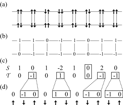
FIG. 7.: Demonstration of topological hidden order in the plaquette-singlet solid state. (a) Spin configuration on each plaquette. Arrows denote the configuration ($\pm\frac{1}{2}$) of $S=\frac{1}{2}$ spins. On each plaquette, the sum of configurations of four spins is restricted to be zero. (b) Spin configuration of corresponding spin-1 ladder. (c) Sequences $\{{\cal S}_{i}\}$ and $\{{\cal T}_{i}\}$ calculated from the configuration (b) as ${\cal S}_{i}=S^{z}_{1,i}+S^{z}_{2,i}$ and ${\cal T}_{i}=S^{z}_{1,i}S^{z}_{2,i}$, respectively. (d) Sequence of ${\cal T}_{i}$’s obtained by being removed elements satisfying both of ${\cal T}_{i}=0$ and $|{\cal S}_{i}|\neq 1$, and replaced 1 and -1 by $(1,0)$ and (-1,0), respectively, in which all positive (negative) ${\cal T}_{i}$’s sit on one (another) sublattice of the sequence.

In Fig. 6, we show the $R$-dependence of our new hidden order parameter,

$$\langle{\cal O}_{4}\rangle_{L}=\frac{1}{L}\sum_{i}\langle{\cal O}_{4}(i,i+L/2)\rangle\,,$$ (30)

calculated for the present model. We plot $\sqrt{\langle{\cal O}_{4}\rangle_{L}}$ instead of $\langle{\cal O}_{4}\rangle_{L}$ itself to demonstrate the relation (29) at $R=0$. In contrast to the conventional string order parameter, $\langle{\cal O}_{2}\rangle_{L}$, which vanishes immediately for $R>0$, the new string order parameter, $\langle{\cal O}_{4}\rangle_{L}$, is found to be a smooth function of $R$, and remains finite up to the dimer limit ($R=1$).

It should be emphasized that although the long-range spin fluctuations are greatly enhanced round $R=0.3$ as discussed in Sec. III, $\langle{\cal O}_{4}\rangle_{L}$ remains remarkably large even in this region. This strongly supports that the ground state of the spin-1 ladder is actually described quite well by the plaquette-singlet solid state (26) in the whole range of $R$.

FIG. 8.: $R$-dependence of the spin gap (open squares) and the inverse correlation length along the chain (solid circles) in the ferromagnetic ($K<0$) case. The dashed lines denote the respective values in the $R\rightarrow-1$ limit (Ref. [13]).

Before closing this section, it might be worth noting that the plaquette-singlet solid state (Eq. (26) and Fig. 5 (c)) has the following topological antiferromagnetic long-range order, though its definition is slightly complicated than its counterpart in the AKLT state for the single spin-1 chain; first, for a given spin configuration $\{S^{z}_{\alpha,j}\}$ ($\alpha=1,2$ and $i=1,2,3,\cdots$), define two sequences, $({\cal S}_{1},{\cal S}_{2},{\cal S}_{3},\cdots)$ and $({\cal T}_{1},{\cal T}_{2},{\cal T}_{3},\cdots)$, where ${\cal S}_{i}$’s and ${\cal T}_{i}$’s are calculated as ${\cal S}_{i}=S^{z}_{1,i}+S^{z}_{2,i}$ and ${\cal T}_{i}=S^{z}_{1,i}S^{z}_{2,i}$, respectively. Next, choose a nearest pair of non-vanishing ${\cal T}_{i}$’s, say ${\cal T}_{j}$ and ${\cal T}_{k}$. If the number of ${\cal S}_{\ell}$’s satisfying $|{\cal S}_{\ell}|=1$ in the interval $j<\ell<k$ is even (odd), then ${\cal T}_{j}$ and ${\cal T}_{k}$ has a same (opposite) sign. In other words, in the sequence of ${\cal T}_{i}$’s, if one removes elements satisfying both of ${\cal T}_{i}=0$ and $|{\cal S}_{i}|\neq 1$, and replaces 1 and -1 by $(1,0)$ and (-1,0), respectively, then one finds the resulting sequence $\{{\cal T}_{i}\}$ has an antiferromagnetic long-range order regarding non-zero elements, i.e., all positive (negative) ${\cal T}_{i}$’s sit on one (another) sublattice of the sequence. A demonstration of this topological order is presented in Fig. 7.

V Ferromagnetic Interchain Coupling

So far, we consider only the case where the interchain coupling is antiferromagnetic ($R>0$). In this section, we consider in turn the ferromagnetic case. In the $R\rightarrow-1$ limit, two $S=1$ spins connected by an infinitely-strong ferromagnetic rung bond form $S=2$. Thus, two intrachain antiferromagnetic coupling of strength $J$ in Eq. (2) are transformed into one bond of strength $\tilde{J}=J/2$ connecting two $S=2$ spins. The spin-2 antiferromagnetic chain has a finite spin gap, $\Delta/\tilde{J}=0.08917(4)$, which is much smaller than that of the spin-1 chain, and also a longer correlation length, $\xi=49.49(1)$. [13]

FIG. 9.: $K/J$-dependence of the spin gap, $\Delta/J$, in the antiferromagnetic ($K>0$) and ferromagnetic ($K<0$) cases. The dotted straight lines are obtained by least-squares fitting for $0\leq K/J<0.025$ and $-0.025<K/J\leq 0$, respectively.

The spin-2 Haldane state is also explained by a VBS picture, in which two dimers sitting on each bond. Therefore, one would expect naturally that the two independent spin-1 Haldane state at $R=0$ and the spin-2 one ($R\rightarrow-1$) is connected smoothly without any singularities between them. Indeed, as shown in Fig. 8, the spin gap, $\Delta/J$, as well as the correlation length, $\xi$, decreases monotonically as $R$ does, and seems to converge smoothly to the values of the spin-2 Haldane chain. Note that the spin gap presented in Fig. 8 is not the reduced gap, $\tilde{\Delta}$. Since $\tilde{\Delta}$ vanishes as $\sim 1/|K|$ for $R\ll 0$, we normalize the gap as $\Delta/J$, which remains finite in the $R\rightarrow-1$ limit. At $R=-0.8$ and $-0.9$, we need $L=512$ and $\tilde{T}=0.0009766$ to obtain the zero-temperature values in the thermodynamic limit.

Although the decoupled-chain point ($K=0$) is not a critical point, the spin gap is still non-analytic at this point. In Fig. 9, we show the $K/J$-dependence of $\Delta/J$ near $K=0$ ($|K/J|\leq 0.01$) both in the antiferromagnetic and ferromagnetic regimes. One sees a clear cusp just at $K=0$. In both regimes, $\Delta/J$ decreases linearly as $|K/J|$ increases. Furthermore, we find the absolute value of its slope is the same within the error on both sides (3.72(3) for $K>0$ and 3.75(3) for $K<0$). We should remark this is completely consistent with the conjecture by the previous bosonization study. [16]

VI Summary and Discussions

In this paper, we investigated precisely the ground-state properties of the spin-1 antiferromagnetic Heisenberg two-leg ladder by means of the quantum Monte Carlo simulation. We found that the system is gapful regardless of the strength of interchain coupling, that is, the Haldane state in the decoupled chains and the spin-1 dimer state are connected smoothly and there is no quantum phase transition between them. We conclude that the behavior of the spin gap as a function of $R$ we observed, including the cusp at $R=0$, is completely consistent with the recent analytic studies based on the mapping to the nonlinear $\sigma$ model [15] and the bosonization technique. [16]

Although there is no quantum phase transition in the present system, the spin gap is greatly suppressed, and at the same time the long-range antiferromagnetic fluctuations are enhanced in the intermediate region ($R\simeq 0.3$), e.g., $\Delta/(J+K)=0.06476(4)$ and $(J+K)\chi_{\rm s}=490.1(2)$ at $R=0.3$. This explains the reason why the spin-1 ladder with $R\simeq 0.3$ exhibits an antiferromagnetic long-range order, if one introduces quite small ($\simeq 0.004J$) antiferromagnetic coupling between ladders. [30] It should be noted that the critical inter-ladder coupling is smaller by an order of magnitude than the spin gap. This situation is the same as the critical interchain coupling, $J^{\prime}_{\rm c}$, of the two-dimensional array of spin-1 chains, $J^{\prime}_{\rm c}/J=0.043648(8)$, [30] while $\Delta/J=0.41050(2)$. [10] The precise ground-state phase diagram of these two-dimensional spin-1 Heisenberg antiferromagnets has been reported in detail in Ref. [30].

The AKLT picture, which works quite well for the single spin-1 chain, was found to break down immediately in the presence of interchain coupling. We proposed the plaquette-singlet solid state to describe the ground state qualitatively for the whole range of $R$. The plaquette-singlet solid state has a topological hidden order. The hidden order parameter $\langle{\cal O}_{4}\rangle$, which characterizes the plaquette-singlet solid state, was shown to be finite up to the dimer limit ($R=1$). This strongly supports that the ground state of the spin-1 ladder is described quite well by the present plaquette-singlet solid picture.

It is quite interesting to see that the local Hamiltonian of spin-$\frac{1}{2}$ plaquette, Eq. (24), itself can reproduce qualitatively correct behavior of the spin gap observed in the present spin-1 ladder. The Hamiltonian (24) has a singlet ground state regardless of the value of $x_{\rm p}\equiv K_{\rm p}/J_{\rm p}$ ($-\infty\leq x_{\rm p}\leq\infty$). The $x_{\rm p}$-dependence of the spin gap can be written explicitly as follows:

$$\frac{\Delta}{J_{\rm p}}=\left\{\begin{array}[]{ll}\sqrt{1-x_{\rm p}+x_{\rm p}^{2}}&\,\,\,\,\mbox{for $x_{\rm p}\geq 0$}\\ x_{\rm p}+\sqrt{1-x_{\rm p}+x_{\rm p}^{2}}&\,\,\,\,\mbox{for $x_{\rm p}\leq 0.$}\\ \end{array}\right.$$ (31)

One can find easily the following features: (i) There always exists a finite gap for $-\infty\leq x_{\rm p}\leq\infty$. (ii) For $x_{\rm p}>0$ ($K_{\rm p}>0$), $\Delta/(J_{\rm p}+K_{\rm p})$ has a minimum at a finite value of $x_{\rm p}$. (iii) On the other hand, for $x_{\rm p}<0$ ($K_{\rm p}<0$), $\Delta/J_{\rm p}$ is a monotonically-decreasing function of $|x_{\rm p}|$, and converges to a finite value at $x_{\rm p}=-\infty$. (iv) Finally, at $x_{\rm p}=0$, $\Delta/J_{\rm p}$ has a cusp, and it decreases linearly with the same slope on both sides. The last behavior is simply due to the crossing of the second- and third-lowest eigenvalues. All of these features are qualitatively the same as the present spin-1 ladder.

The plaquette-singlet solid picture proposed in the present paper might be generalized to wider classes of the spin-1 Heisenberg ladder. Indeed, for the ferromagnetic interchain coupling case discussed in Sec. V, our hidden order parameter $\langle O_{4}\rangle$ was found to remain at a finite value ($\simeq 0.089$) in the limit $K\rightarrow-\infty$. Furthermore, the present plaquette-singlet solid picture might be applied even in the presence of bond alternation (forced dimerization) in the intrachain coupling, i.e., $J_{i}=(1+(-1)^{i}\delta)J$, where $\delta$ denotes the strength of dimerization. We have observed that there is no singularity for the whole range of $\delta$ ($0\leq\delta\leq 1$), and $\langle O_{4}\rangle$ remains finite up to the decoupled-plaquette limit ($\delta=1$). Note that as for the decoupled dimerized chain ($K=0$), the $\delta$-dependence of $\langle O_{4}\rangle$ is qualitatively different from that for $K>0$. There exists a critical point at $\delta_{\rm c}=0.26001(4)$, [31] and the conventional string order parameter $\langle O_{2}\rangle$ vanishes for $\delta\geq\delta_{\rm c}$. Since the relation (29) holds for $K=0$, the new hidden order parameter $\langle O_{4}\rangle$ also vanishes for $\delta\geq\delta_{\rm c}$. The existence of non-zero hidden order parameter $\langle O_{4}\rangle$ in the cases with ferromagnetic couplings and with alternating bonds implies their ground states are also well described by products of local singlet states similar to the present plaquette-singlet solid state, though the structure of local singlet state should be quite different from the present one.

Very recently a new nitroxide material, abbreviated as BIP-TENO, has been synthesized, and its magnetic properties have been investigated precisely. [32, 33] The tetraradical BIP-TENO molecule consists of two pairs of ferromagnetically-coupled $S=\frac{1}{2}$ spins, and relatively weak antiferromagnetic coupling exists between the pairs. The crystalline state of BIP-TENO is thus expected to be described effectively by a spin-1 antiferromagnetic ladder of present interest. From the high-temperature behavior of the uniform susceptibility, Katoh et al. estimated the strength of effective couplings and concluded that $J\simeq 50{\rm K}$ and $K\simeq 42{\rm K}$, i.e., $R\simeq 0.46$.[32] A clear spin-gapped behavior of the uniform susceptibility observed in the experiment is consistent with the present results. The excitation gap $\Delta$ is also estimated to be 15.6K from the magnetization curve. [33] Unfortunately, its magnitude is more than twice as large as the present result ($\Delta/(J+K)=0.07392(6)$ at $R=0.45$. See Fig. 4).

Interestingly, the shoulder in the temperature dependence of the uniform susceptibility (Fig. 2) has also been observed even in the real material. [32] This anomaly in the excitation spectrum might be related with the $\frac{1}{4}$-plateau observed in the magnetization process of BIP-TENO. [33] However, it is beyond the scope of the present study, and remains as a future problem.

REFERENCES

- [1] Electronic address: wistaria@itp.phys.ethz.ch
- [2] Electronic address: matumoto@issp.u-tokyo.ac.jp
- [3] Electronic address: cyasuda@issp.u-tokyo.ac.jp
- [4] Electronic address: takayama@issp.u-tokyo.ac.jp
- [5] For reviews, see e.g., E. Dagotto and T. M. Rice, Science 271, 618 (1996); E. Dagotto, Rep. Prog. Phys. 62, 1525 (1999).
- [6] F. D. M. Haldane, Phys. Lett. 93A, 464 (1983); Phys. Rev. Lett. 50, 1153 (1983).
- [7] I. Affleck, T. Kennedy, E. H. Lieb, and H. Tasaki, Phys. Rev. Lett. 59, 799 (1987).
- [8] M. den Nijs and K. Rommelse, Phys. Rev. B 40, 4709 (1989).
- [9] M. P. Nightingale and H. W. J. Blöte, Phys. Rev. B 33, 659 (1986).
- [10] S. R. White and D. A. Huse, Phys. Rev. B 48, 3844 (1993).
- [11] O. Golinelli, Th. Jolicœur, and R. Lacaze, Phys. Rev. B 50, 3037 (1994).
- [12] U. Schollwöck and Th. Jolicœur, Europhys. Lett. 30, 493 (1995).
- [13] S. Todo and K. Kato, to appear in Phys. Rev. Lett. (cond-mat/9911047).
- [14] K. Totsuka and M. Suzuki, J. Phys.: Condens. Matter 7, 6079 (1995).
- [15] D. Sénéchal, Phys. Rev. B 52, 15319 (1995).
- [16] D. Allen and D. Sénéchal, Phys. Rev. B 61, 12134 (2000).
- [17] H. G. Evertz, G. Lana, and M. Marcu, Phys. Rev. Lett. 70, 875 (1993)
- [18] U.-J. Wiese and H.-P. Ying, Z. Phys. B: Condens. Matter 93, 147 (1994)
- [19] B. B. Beard and U.-J. Wiese, Phys. Rev. Lett. 77, 5130 (1996).
- [20] M. Suzuki, Quantum Monte Carlo Methods in Condensed Matter Physics (World Scientific, Singapore, 1994), and references therein.
- [21] For reviews, see e.g., H. G. Evertz, unpublished (cond-mat/9707221).
- [22] N. Kawashima and J. E. Gubernatis, Phys. Rev. Lett. 73, 1295 (1994); J. Stat. Phys. 80, 169 (1995).
- [23] K. Harada, M. Troyer, and N. Kawashima, J. Phys. Soc. Jpn. 67, 1130 (1998).
- [24] F. Cooper, B. Freedman, and D. Preston, Nucl. Phys. B 210 [FS6], 210 (1982).
- [25] An interesting extension of the loop algorithm, which works directly in the thermodynamic limit, has been proposed in H. G. Evertz and W. von der Linden, preprint (cond-mat/0008072).
- [26] Here, we assume the Lorentz invariance, i.e., the dynamical exponent is unity.
- [27] This argument does not apply for the equal-time quantities, such as the static structure factor (8). Since we measured them only at , is merely proportional to instead of .
- [28] S. Todo, K. Kato, and H. Takayama, J. Phys. Soc. Jpn. Suppl. A 69, 355 (2000).
- [29] Direct products of plaquette singlets were also used in Ref. [14] as a starting point of the perturbation expansion for the spin- forced-dimerized two-leg ladder.
- [30] M. Matsumoto, C. Yasuda, S. Todo, and H. Takayama, preprint.
- [31] M. Nakamura, J. Voit, and S. Todo, unpublished.
- [32] K. Katoh, Y. Hosokoshi, K. Inoue, and T. Goto, J. Phys. Soc. Jpn. 69, 1008 (2000).
- [33] T. Goto, M. I. Bartashevich, Y. Hosokoshi, K. Kato, and K. Inoue, Physica B 294-295, 43 (2001).