Critical Point of a Weakly Interacting Two-Dimensional Bose Gas

Abstract

We study the Berezinskii–Kosterlitz–Thouless transition in a weakly interacting 2D quantum Bose gas using the concept of universality and numerical simulations of the classical $|\psi|^{4}$-model on a lattice. The critical density and chemical potential are given by relations $n_{c}=(mT/2\pi\hbar^{2})\ln(\xi\hbar^{2}/mU)$ and $\mu_{c}=(mTU/\pi\hbar^{2})\ln(\xi_{\mu}\hbar^{2}/mU)$, where $T$ is the temperature, $m$ is the mass, and $U$ is the effective interaction. The dimensionless constant $\xi=380\pm 3$ is very large and thus any quantitative analysis of the experimental data crucially depends on its value. For $\xi_{\mu}$ our result is $\xi_{\mu}=13.2\pm 0.4$. We also report the study of the quasi-condensate correlations at the critical point.

An accurate microscopic expression for the critical temperature of the Berezinskii–Kosterlitz–Thouless (BKT) transition [1] has been a weak point of the theory of weakly interacting two-dimensional Bose gas. The theory of Ref.  [2] (see also [3, 4] and analysis below), suggests that the critical density of the BKT transition in the weakly interacting system reads (we set $\hbar=1$)

$$n_{c}={mT\over 2\pi}\ln{\xi\over mU}\;.$$ (1)

However, the value of $\xi$ cannot be obtained within standard analytical treatments since $\xi$ is related to the system behavior in the fluctuation region where the perturbative expansion in powers of $U$ does not work. With unknown $\xi$, one finds Eq. (1) rather inaccurate unless $mU$ is exponentially small. Moreover, as we will find in this Letter, the value of $\xi$ is very large: $\xi\approx 380$. This means that for all experimentally available up to date (quasi-)2D weakly interacting Bose gases [5, 6] the quantitative analysis of the data for the critical ratio $n_{c}/T_{c}$ requires a precise value of $\xi$. In the system of spin-polarized atomic hydrogen on helium film [5], the value of $mU$ is of order unity [3]; in the recently created quasi-2D system of sodium atoms [6], $mU$ is of order $10^{-2}$, according to the formula of Ref. [7].

To quantitatively describe the BKT transition in a weakly interacting Bose gas, it is sufficient to solve a classical-field $|\psi|^{4}$-model with the effective long-wave Hamiltonian [2]

$$H[\psi]=\int\left\{{1\over 2m}|\nabla\psi|^{2}+{U\over 2}|\psi|^{4}-\mu^{\prime}|\psi|^{2}\right\}\,d{\bf r}\;,$$ (2)

where $\mu^{\prime}$ is the chemical potential, and $\psi$ is the classical complex field.

In this Letter, we first discuss the origin of the relation (1) in the limit of small $U$, and how quantum and classical models relate to each other. Then we present our numeric results (for the critical density, critical chemical potential, and quasi-condensate correlations at the BKT point) obtained by simulating the critical behavior of the 2D $|\psi|^{4}$-model on a lattice using recently developed Worm algorithm [8] for classical statistical models. In particular, we show that the quasi-condensate correlations are very strong at $T_{c}$, in agreement with the experimental observation in the spin-polarized atomic hydrogen [5] and quantum Monte Carlo simulations [9].

A simple dimensional analysis of the Hamiltonian (2) allows to write a generic formula for the critical point in a weakly interacting 2D $|\psi|^{4}$-model. The routine itself is completely analogous to that in the 3D case (see, e.g., [10, 11]), but final results naturally reflect the specifics of the 2D case.

We begin with introducing the mode-coupling momentum, $k_{c}$, that characterizes the onset of strong non-linear coupling between the long-wave harmonics of $\psi({\bf r})$ (harmonics with $k\gg k_{c}$ are almost free). This momentum is just the inverse of the healing length, or vortex core radius, $r_{c}$  [1]. We denote by $\tilde{n}$ the contribution to the total density due to strongly coupled harmonics, and introduce the renormalized chemical potential

$$\tilde{\mu}=\mu^{\prime}-2U\int_{k>k_{c}}n_{k}^{\rm(ideal)}d^{2}k/(2\pi)^{2}$$ (3)

by subtracting the mean field contribution of non-interacting high-momentum harmonics. Here $n_{k}=\langle\,|\psi_{\bf k}|^{2}\rangle$, and $\langle\ldots\rangle$ stands for the statistical averaging.

An estimate for $\tilde{n}$ follows from the Nelson-Kosterlitz formula

$$n_{s}={2mT\over\pi}\;,$$ (4)

since it is intuitively expected that $\tilde{n}\sim n_{s}$. An independent estimate of the parameters of the fluctuation region is obtained by considering when all three terms in Eq. (2) are of the same order:

$$k_{c}^{2}/m\sim|\tilde{\mu}|\sim\tilde{n}U\;,$$ (5)

and relating $\tilde{n}\sim\sum_{k<k_{c}}n_{k}\sim k_{c}^{2}n_{k_{c}}$ to the renormalized chemical potential by using $T/|\tilde{\mu}|$ in place of the occupation number $n_{k_{c}}$. By definition, $k_{c}$ separates strongly coupled and free harmonics, and thus $n_{k_{c}}\sim T/[k_{c}^{2}/2m-\tilde{\mu}]\sim T/|\tilde{\mu}|$. The final order-of-magnitude estimates read (at $T=T_{c}$)

$$\tilde{n} \sim mT\;,$$ (6)

$$k_{c} \sim m(UT)^{1/2}\;,$$ (7)

$$\tilde{\mu} \sim UmT\;.$$ (8)

We are now in a position to derive Eq. (1) for the critical density. In 2D the main contribution to the integral

$$n=\int n_{k}d^{2}k/(2\pi)^{2}\;,$$ (9)

comes from large momenta between $k_{c}$ and some ultra-violet scale $k_{*}$. The value and physical meaning of $k_{*}$ depend on the model. For classical lattice models $k_{*}$ is given by the inverse lattice spacing; in the continuous quantum system $k_{*}\sim\sqrt{mT}$ is the thermal momentum. At $k_{c}\ll k\ll k_{*}$ we have $n_{k}\approx 2mT/k^{2}$, and thus can write

$$n_{c}={mT\over 2\pi}\ln(Ck_{*}^{2}/k_{c}^{2})\;,$$ (10)

where $C$ is some constant. Critical density, Eq. (1), for the quantum Bose gas is obtained by substituting $Ck_{*}^{2}/k_{c}^{2}\equiv\xi mT/m^{2}UT=\xi/mU$.

The dependence on the ultraviolet cutoff is associated with the properties of ideal systems only, while the long-wave behavior of all weakly-interacting $|\psi|^{4}$-theories is universal. This fact allows one to relate results for different models by adding and subtracting non-interacting contributions, i.e., up to higher order corrections in $U$ the difference between models ${\cal A}$ and ${\cal B}$ is given by $(n_{c}^{\cal(A)}-n_{c}^{\cal(B)})=\int[n_{k}^{\rm(ideal~{}{\cal A})}-n_{k}^{\rm(ideal~{}{\cal B})}]\,d^{2}k/(2\pi)^{2}$. In what follows, the reference system ${\cal A}$ will be the classical lattice model with lattice spacing $a$, and our results are analyzed using

$$n_{c}^{\rm(lat)}={mT\over 2\pi}\ln{A\over m^{2}a^{2}UT}\;.$$ (11)

The actual system of interest is the quantum Bose gas, so we add and subtract the corresponding ideal-system contributions to get

$$\ln{A\over\xi ma^{2}T}={1\over 2\pi mT}\left(\int_{BZ}{T~{}d^{2}k\over E({\bf k})}-\int{d^{2}k\over e^{k^{2}/2mT}-1}\right)\;,$$ (12)

where $BZ$ means that the first integral is over the Brillouin zone, and $E({\bf k})$ is the dispersion law for the ideal lattice model such that $E({\bf k}\to 0)\to k^{2}/2m$. [The divergences of the two integrals in Eq. (12) at $k\to 0$ compensate each other.]

Our simulations were done for the simple square lattice Hamiltonian

$$H=\sum_{{\bf k}\in BZ}[E({\bf k})-\mu]|\psi_{k}|^{2}+{U\over 2}\sum_{i}|\psi_{i}|^{4}\;,$$ (13)

where $\psi_{k}$ is the Fourier transform of the complex lattice field $\psi_{i}$, and

$$E({\bf k})=(1/ma^{2})[2-\cos(k_{x}a)-\cos(k_{y}a)]$$ (14)

is the tight-binding dispersion law. With this dispersion relation the r.h.s. in (12) can be evaluated analytically and we obtain the “conversion” formula

$$\xi=A/16\;.$$ (15)

Since final results for dimensionless constants do not depend on $m$, $T$, and $a$, in numerical simulations we set $a=1$, $T=1$, and $m=1/2$ for convenience.

The above consideration for the critical density can be readily generalized to the critical chemical potential, with the result

$$\mu_{c}={mTU\over\pi}\ln{\xi_{\mu}\over mU}\;.$$ (16)

First, we notice that Eq. (16) immediately follows form Eqs. (8) and Eq. (3) because the mean-field term is proportional to $-(mUT/\pi)\ln(mU)$ (we actually deal with exactly the same integral). Since the renormalized value $\tilde{\mu}$ is universal, to account for the difference between the classical and quantum models one has to add and subtract mean-field contributions dominated by the ideal behavior. Thus, if the classical model is analyzed using $\mu_{c}=(mTU/\pi)\ln[A_{\mu}/m^{2}a^{2}UT]$, one has to apply $\xi_{\mu}=A_{\mu}/16$ to get the quantum result, Eq. (16).

We now turn to our numerical procedure. To simulate the grand-canonical Gibbs distribution corresponding to the Hamiltonian (13), we employ the Worm algorithm (see Ref. [8] for the description) that has demonstrated its efficiency for the analogous problem in 3D [11]. The formal criterion of the critical point for the finite-size system is based on the exact (Nelson–Kosterlitz) relation (4): We say that the system of linear size $L$ is at the critical point, if its superfluid density, $n_{s}(L)$, satisfies $n_{s}(L)=2mT/\pi$. [The superfluid density has a direct estimator in the Worm algorithm via the statistics of winding numbers [8], and its autocorrelation time does not suffer from critical slowing down.]

The finite size scaling of $n_{c}(L)$ is well known from the Kosterlitz-Thouless renormalization group theory [1]

$$n_{c}(L)=n_{c}-\frac{A^{\prime}\,mT}{\ln^{2}\big{[}A^{\prime\prime}\,Lm(UT)^{1/2}\big{]}}\;,$$ (17)

where $A^{\prime}$ and $A^{\prime\prime}$ are dimensionless constants. A similar relation applies also to the critical chemical potential. Equation  (17) was used for the finite-size scaling analysis. We found that instead of extrapolating data for each value of $U$ to the $L\to\infty$ limit independently, a much more efficient procedure is to perform a joint finite-$L$ and finite-$U$ analysis. To this end we heuristically introduce parameters accounting for non-universal finite-$U$ corrections by adding linear in $U$ terms to each of the three of the dimensionless constants: $A\to A+BU$, $A^{\prime}\to A^{\prime}+B^{\prime}U$, and $A^{\prime\prime}\to A^{\prime\prime}+B^{\prime\prime}U$. We thus have six fitting parameters to describe all our data points [13]. The data for $n_{c}(U,L)$ and $\mu_{c}(U,L)$ are presented in Fig. 1. The fitting procedure yields $A=(6.07\pm 0.05)\cdot 10^{3}$, $A_{\mu}=(211\pm 6)$, which, according to Eq. (15), means that

$$\xi=380\pm 3\;,~{}~{}~{}~{}~{}\xi_{\mu}=13.2\pm 0.4\;.$$ (18)

The fit is extremely good—20 points for the critical density at $U\leq 2.5$ and $Lm(UT)^{1/2}>15$, each calculated with relative accuracy of order $10^{-4}$, are described with the confidence level of $62$ %.

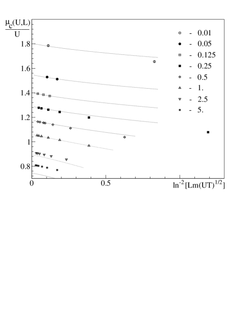
FIG. 1.: Critical density and chemical potential for various coupling parameters and system sizes. Typical error bars are much smaller than symbol sizes. The dotted line is the fitting function described in the text.

Experiments on helium films often report that the ratio $n_{s}(T_{c})/n_{s}(0)=n_{s}(T_{c})/n_{c}=2mT_{c}/\pi n_{c}$ is close to $0.75$ [14, 15]. Our simulation predicts that this ratio is given by

$$n_{s}(T_{c})/n_{c}={4\over 5.94-\ln(mU)}\;,$$ (19)

and $mU\approx 1.8$ is required to describe helium films, provided the small-$U$ approximation may be pushed that far [16]. We are not aware of the published data on the critical chemical potential. [For helium and hydrogen films on substrates one has to shift $\mu_{c}$ by the value of the absorption energy (for the delocalized atom, in the case of helium film), $\mu_{c}\to\mu_{c}=E_{0}+(mTU/\pi)\ln(\xi_{\mu}/mU)$. In thermal equilibrium this quantity can be readily measured through the chemical potential of the bulk vapor.]

In the absence of long-range order parameter, 2D systems below $T_{c}$ are characterized by the local correlation properties of the quasicondensate density, identical to those of a system with genuine condensate [3]. These properties reflect the specific structure of the $\psi$-field:

$$\psi({\bf r}) = \psi_{0}({\bf r})+\psi_{1}({\bf r})\;,$$ (20)

$$\psi_{0}({\bf r}) \approx \sqrt{n_{0}}\,e^{i\Phi({\bf r})}\;,$$ (21)

where the quasicondensate density $n_{0}$ may be considered as a constant, and $\psi_{1}$ is the Gaussian field independent of $\psi_{0}$. Both experiment [5] and model Monte Carlo simulations [9] indicate that in 2D systems with $mU\sim 1$ the quasicondensate correlations appear well above $T_{c}$ and are pronounced at $T_{c}$. Below we show that this is a generic feature of weakly interacting $|\psi|^{4}$-models.

It is convenient to characterize the quasi-condensate properties by the correlator

$$Q=2\langle\,|\psi|^{2}\rangle^{2}-\langle\,|\psi|^{4}\rangle\;.$$ (22)

The Gaussian component of the field obeys the Wick’s theorem and does not contribute to Eq. (22). If, for a moment, by $\psi_{1}$ we understand short-wave harmonics of $\psi$, we conclude that only long-wave and strongly non-linear harmonics with the momenta $k\sim k_{c}$ contribute to the correlator $Q$, i.e. $Q\sim\tilde{n}^{2}$. Thus, we expect that all weakly interacting $|\psi|^{4}$-models satisfy

$$Q=C_{*}m^{2}T^{2}~{}~{}~{}~{}~{}~{}~{}(T=T_{c})$$ (23)

in the limit of small $U$, where $C_{*}$ is a universal constant. By definition, $n_{0}=\sqrt{Q}$.

The finite-size and small-$U$ analysis of the data for $Q(U,L)$ was done in complete analogy with previously discussed cases of $n_{c}(U,L)$ and $\mu_{c}(U,L)$ (see Ref. [13]). We found that

$$C_{*}=1.30\pm 0.02$$ (24)

The ratio between $n_{0}(T=T_{c})$ and $n_{c}$ describes how pronounced are the quasicondensate correlations in the Bose gas at the BKT point:

$${n_{0}^{(T=T_{c})}\over n_{c}}={2\pi\sqrt{C_{*}}\over\ln(\xi/mU)}={7.16\over 5.94+\ln(1/mU)}\;.$$ (25)

We see, that it is of order unity unless $mU$ is exponentially small. Another interesting ratio is

$${n_{0}\over n_{s}}={\pi\sqrt{C_{*}}\over 2}\approx 1.79~{}~{}~{}~{}~{}~{}~{}(T=T_{c})\;,$$ (26)

which is interaction independent and shows that the superfluid density is substantially smaller than the quasicondensate density at $T_{c}$.

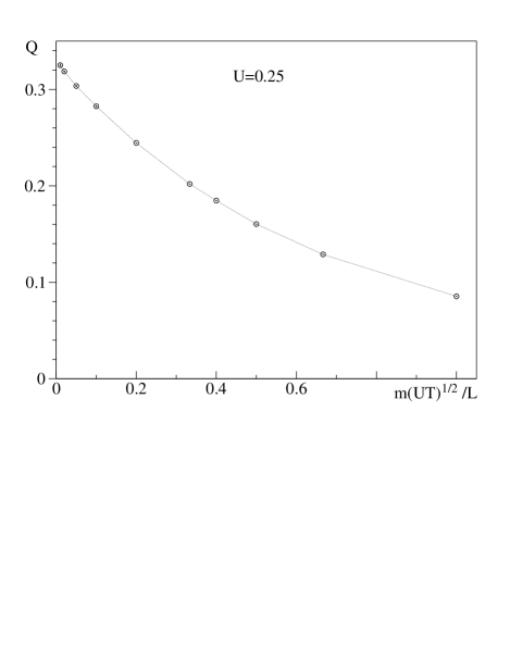
FIG. 2.: Quasicondensate correlations as a function of system size. The dotted line is to guide the eye.

Finally, we would like to derive an accurate estimate for the mode-coupling radius $r_{c}$. In an ideal system $Q\equiv 0$. Hence, $Q(L)$ should decrease with decreasing $L$, and for system sizes $L\sim r_{c}$ it has to drop significantly from its thermodynamic value. We rather formally define $r_{c}$ from $Q(L=r_{c})\approx Q(L\to\infty)/2$, and from Fig. 2 obtain

$$r_{c}\approx 2/m(UT)^{1/2}\;.$$ (27)

We conclude by noting that Nelson-Kosterlitz formula (4) and Eqs. (1), (16), and (23) constitute a complete set of equations which allow to fully determine system parameters from measurements with independent cross-checks. We are not aware of another study were dimensionless constants $\xi$, $\xi_{\mu}$, and $C_{*}$ were determined with high precision.

We thank J. Machta and R. Hallock for valuable discussions. This work was supported by the National Science Foundation under Grant DMR-0071767. BVS acknowledges a support from Russian Foundation for Basic Research under Grant 01-02-16508.

REFERENCES

- [1] V.L. Berezinskii, Sov. Phys. JETP 32, 493 (1971); 34, 610 (1972); J.M. Kosterlitz and D.J. Thouless, J. Phys. C 6, 1181 (1973); J.M. Kosterlitz, J. Phys. C 7, 1046 (1974).
- [2] V.N. Popov, Functional Integrals in Quantum Field Theory and Statistical Phisics (Reidel, Dordrecht, 1983).
- [3] Yu. Kagan, B.V. Svistunov, and G.V. Shlyapnikov, Sov. Phys. - JETP 66, 314 (1987).
- [4] D.S. Fisher and P.C. Hohenberg, Phys. Rev. B 37, 4936 (1988).
- [5] A.I. Safonov, S.A. Vasilyev, I.V. Yasnikov, I.I. Lukashevich, and S. Jaakkola, Phys. Rev. Lett. 81, 4545 (1998).
- [6] A. Görlitz et al., cond-mat/0104549.
- [7] D.S. Petrov, M. Holzmann, and G.V. Shlyapnikov, Phys. Rev. Lett. 84, 2551 (2000).
- [8] N.V. Prokof’ev, and B.V. Svistunov, cond-mat/0103146.
- [9] Yu. Kagan, V.A. Kashurnikov, A.V. Krasavin, N.V. Prokof’ev, and B.V. Svistunov, Phys. Rev. A 61, 4360 (2000).
- [10] G. Baym, J.-P. Blaizot, M. Holzmann, F. Laloë, and D. Vautherin, Phys. Rev. Lett. 83, 1703 (1999).
- [11] V.A. Kashurnikov, N.V. Prokof’ev, and B.V. Svistunov, cond-mat/0103149.
- [12] D.R. Nelson and J.M. Kosterlitz, Phys. Rev. Lett. 39, 1201 (1977).
- [13] Fitting parameters are obtained from the stochastic optimization procedure. The error bars are estimated from fluctuations observed when some of the points are added/removed from the optimization. We have also tried to look for the non-universal finite- corrections of the form , but, within the error bars, obtained the same result for , and . On another hand, corrections were important in the fit for .
- [14] G. Agnolet, D.F. McQueeney, and J.D. Reppy, Phys. Rev. B 39, 8934 (1989).
- [15] P.S. Ebey, P.T. Finley, and R.B. Hallock, J. Low Temp. Phys. 110, 635 (1998).
- [16] Actually, the interaction is too large for a quantum Bose system to be accurately described as a weakly interacting gas. From our estimate for the mode-coupling radius, Eq. (27), we see that at such interactions is already on the order of the interparticle distance. Also, Eq. (25) makes no sense at all for .