Learning curves for Gaussian process regression: Approximations and bounds

Abstract

We consider the problem of calculating learning curves (i.e., average generalization performance) of Gaussian processes used for regression. On the basis of a simple expression for the generalization error, in terms of the eigenvalue decomposition of the covariance function, we derive a number of approximation schemes. We identify where these become exact, and compare with existing bounds on learning curves; the new approximations, which can be used for any input space dimension, generally get substantially closer to the truth. We also study possible improvements to our approximations. Finally, we use a simple exactly solvable learning scenario to show that there are limits of principle on the quality of approximations and bounds expressible solely in terms of the eigenvalue spectrum of the covariance function.

1 Introduction: Gaussian processes

Within the neural networks community, there has in the last few years been a good deal of excitement about the use of Gaussian processes as an alternative to feedforward networks (see e.g. Williams and Rasmussen (1996); Williams (1997); Barber and Williams (1997); Goldberg et al. (1998); Sollich (1999a); Malzahn and Opper (2001). The advantages of Gaussian processes are that prior assumptions about the problem to be learned are encoded in a very transparent way, and that inference—at least in the case of regression that we will consider—is relatively straightforward; they are also ‘non-parametric’ in the sense that their effective number of parameters (‘degrees of freedom’) can grow arbitrarily large as more and more training data is collected.

One crucial question for applications is then how ‘fast’ Gaussian processes learn, i.e., how many training examples are needed to achieve a certain level of generalization performance. The typical (as opposed to worst case) behaviour is captured in the learning curve, which gives the average generalization error $\epsilon$ as a function of the number of training examples $n$. Several workers have derived bounds on $\epsilon(n)$ Michelli and Wahba (1981); Plaskota (1990); Opper (1997); Trecate et al. (1999); Opper and Vivarelli (1999); Williams and Vivarelli (2000) or studied its large $n$ asymptotics Silverman (1985); Ritter (1996). As we will illustrate below, however, the existing bounds are often far from tight; and asymptotic results will not necessarily apply for realistic sample sizes $n$. Our main aim in this paper is therefore to derive approximations to $\epsilon(n)$ which get closer to the true learning curves than existing bounds, and apply both for small and large $n$. We compare these approximations with existing bounds and the results of numerical simulations; possible improvements to the approximations are also discussed. Finally, we study an analytically solvable example scenario which sheds light on how tight bounds on learning curves can be made in principle. Summaries of the early stages of this work have appeared in the conference proceedings Sollich (1999a, b).

In its simplest form, the regression problem that we are considering is this: We are trying to learn a function $\theta^{*}$ which maps inputs $x$ (real-valued vectors) to (real-valued scalar) outputs $\theta^{*}(x)$. We are given a set of training data $D$, consisting of $n$ input-output pairs $(x_{l},y_{l})$; the training outputs $y_{l}$ may differ from the ‘clean’ target outputs $\theta^{*}(x_{l})$ due to corruption by noise. Given a test input $x$, we are then asked to come up with a prediction $\theta(x)$ for the corresponding output, expressed either in the simple form of a mean prediction $\hat{\theta}(x)$ plus error bars, or more comprehensively in terms of a ‘predictive distribution’ $P(\theta(x)|x,D)$. In a Bayesian setting, we do this by specifying a prior $P(\theta)$ over our hypothesis functions, and a likelihood $P(D|\theta)$ with which each $\theta$ could have generated the training data; from this we deduce the posterior distribution $P(\theta|D)\propto P(D|\theta)P(\theta)$. If we wanted to use a feedforward network for this task, we could proceed as follows: Specify candidate networks by a set of weights $w$, with prior probability $P(w)$. Each network defines a (stochastic) input-output relation described by the distribution of output $y$ given input $x$ (and weights $w$), $P(y|x,w)$. Multiplying over the whole data set, we get the probability of the observed data having been produced by the network with weights $w$: $P(D|w)=\prod_{l=1}^{n}P(y_{l}|x_{l},w)$. Bayes’ theorem then gives us the posterior, i.e., the probability of network $w$ given the data, as $P(w|D)\propto P(D|w)P(w)$ up to an overall normalization factor. From this, finally, we get the predictive distribution $P(y|x,D)=\int dwP(y|x,w)P(w|D)$. This solves the regression problem in principle, but leaves us with a nasty integral over all possible network weights: the posterior $P(w|D)$ generally has a highly nontrivial structure, with many local peaks (corresponding to local minima in the training error). One therefore has to use sophisticated Monte Carlo integration techniques Neal (1993) or local approximations to $P(w|D)$ around its maxima MacKay (1992) to tackle this problem. Even once this has been done, one is still left with the question of how to interpret the results: We may for example want to select priors on the basis of the data, e.g. by making the prior $P(w|h)$ dependent on a set of hyperparameters $h$ and choosing $h$ such as to maximize the probability $P(D|h)$ of the data. Once we have found the ‘optimal’ prior we would then hope that it tells us something about the regression problem at hand (whether certain input components are irrelevant, for example). This would be easy if the prior told us directly how likely certain input-output functions are; instead we have to extract this information from the prior over weights, often a complicated process.

By contrast, for a Gaussian process it is an almost trivial task to obtain the posterior and the predictive distribution (see below). One reason for this is that the prior $P(\theta)$ is defined directly over input-output functions $\theta$. How is this done? Any $\theta$ is uniquely determined by its output values $\theta(x)$ for all $x$ from the input domain, and for a Gaussian process, these are simply assumed to have a joint Gaussian distribution (hence the name). This distribution can be specified by the mean values $\left\langle\theta(x)\right\rangle_{\theta}$ (which we assume to be zero in the following, as is commonly done), and the covariances $\left\langle\theta(x)\theta(x^{\prime})\right\rangle_{\theta}=C(x,x^{\prime})$; $C(x,x^{\prime})$ is called the covariance function of the Gaussian process. It encodes in an easily interpretable way prior assumptions about the function to be learned. Smoothness, for example, is controlled by the behaviour of $C(x,x^{\prime})$ for $x^{\prime}\to x$: The Ornstein-Uhlenbeck (OU) covariance function $C(x,x^{\prime})\propto\exp(-||x-x^{\prime}||/l)$ produces very rough (non-differentiable) functions, while functions sampled from the radial basis function (RBF) prior with $C(x,x^{\prime})\propto\exp[-||x-x^{\prime}||^{2}/(2l^{2})]$ are infinitely differentiable. (Intermediate priors yielding $r$ times differentiable functions can also be defined by using modified Bessel functions as covariance functions; see Williams and Vivarelli (2000).) Figure 1 illustrates these characteristics with two samples from the OU and RBF priors, respectively, over a two-dimensional input domain. The ‘length scale’ parameter $l$ in the covariance functions also has an intuitive meaning: It corresponds directly to the distance in input space over which we expect our function to vary significantly. More complex properties can also be encoded; by replacing $l$ with different length scales for each input component, for example, relevant (small $l$) and irrelevant (large $l$) inputs can be distinguished.

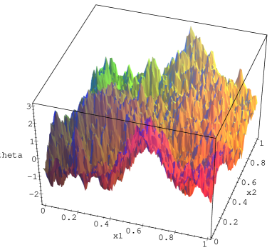
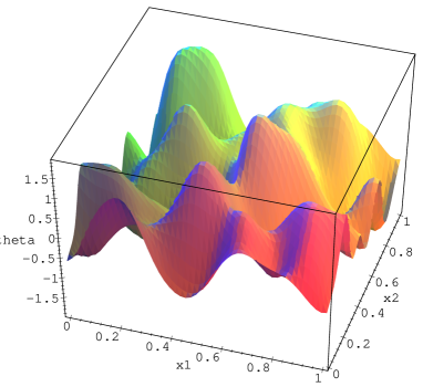
Figure 1: Samples drawn from Gaussian process priors over functions on $[0,1]^{2}$. Left: OU covariance function, $C(x,x^{\prime})=\exp(-||x-x^{\prime}||/l)$. Right: RBF covariance function, $C(x,x^{\prime})=\exp[-||x-x^{\prime}||^{2}/(2l^{2})]$. The length scale $l=0.1$ determines in both cases over what distance the functions vary significantly. Note the difference in roughness of the two functions; this is related to the behaviour of the covariance functions for $x\to x^{\prime}$.

How does inference with Gaussian processes work? We only give a brief summary here and refer to existing reviews on the subject (see e.g. Williams (1998)) for details. It is simplest to assume that outputs $y$ are generated from the ‘clean’ values of a hypothesis function $\theta(x)$ by adding Gaussian noise of $x$-independent variance $\sigma^{2}$. The joint distribution of a set of $n$ training outputs $\{y_{l}\}$ and the function values $\theta(x)$ is then also Gaussian, with covariances given by

$$\left\langle y_{l}y_{m}\right\rangle = C(x_{l},x_{m})+\sigma^{2}\delta_{lm}=({\mathbf{K}})_{lm}$$

$$\left\langle y_{l}\theta(x)\right\rangle = C(x_{l},x)\ \ =\ \ ({\mathbf{k}}(x))_{l}$$

where we have defined an $n\times n$ matrix ${\mathbf{K}}$ and an $x$-dependent $n$-component vector ${\mathbf{k}}(x)$. The posterior distribution $P(\theta|D)$ is then obtained by simply conditioning on the $\{y_{l}\}$. It is again Gaussian and has mean

$$\hat{\theta}(x,D)\equiv\left\langle\theta(x)\right\rangle_{\theta|D}={\mathbf{k}}(x)^{\mathrm{T}}{\mathbf{K}}^{-1}{\mathbf{y}}$$ (1)

and variance

$$\epsilon(x,D)\equiv\left\langle(\theta(x)-\hat{\theta}(x))^{2}\right\rangle_{\theta|D}=C(x,x)-{\mathbf{k}}(x)^{\mathrm{T}}{\mathbf{K}}^{-1}{\mathbf{k}}(x).$$ (2)

Eqs. (1,2) solve the inference problem for Gaussian process: They provide us directly with the predictive distribution $P(\theta(x)|x,D)$. The posterior variance, eq. (2), in fact also gives us the expected generalization error (or Bayes error) at $x$. Why? If the teacher is $\theta^{*}$, the squared deviation between our mean prediction and the teacher output is $(\hat{\theta}(x)-\theta^{*}(x))^{2}$; averaging this over the posterior distribution of teachers $P(\theta^{*}|D)$ just gives (2). The underlying assumption is that our assumed Gaussian process prior is the true one from which teachers are actually generated (and that we are using the correct noise model). Otherwise, the expected generalization error is larger and given by a more complicated expression Williams and Vivarelli (2000). In line with most other work on the subject, we only consider the ‘correct prior’ case in the following. Averaging the generalization error at $x$ over the distribution of inputs gives then

$$\epsilon(D)=\left\langle\epsilon(x,D)\right\rangle_{x}=\left\langle C(x,x)-{\mathbf{k}}(x)^{\mathrm{T}}{\mathbf{K}}^{-1}{\mathbf{k}}(x)\right\rangle_{x}$$ (3)

This form of the generalization error, which is well known Michelli and Wahba (1981); Opper (1997); Williams (1998); Williams and Vivarelli (2000), still depends on the training inputs; the fact that the training outputs have dropped out already is a signature of the fact that Gaussian processes are linear predictors (compare (1)). Averaging over data sets yields the quantity we are after,

$$\epsilon=\left\langle\epsilon(D)\right\rangle_{D}.$$ (4)

This average expected generalization error (we will drop the ‘average expected’ in the following) only depends on the number of training examples $n$; the function $\epsilon(n)$ is called the learning curve. Its exact calculation is difficult because of the joint average in eqs. (3,4) over the training inputs $x_{l}$ and the test input $x$.

Before proceeding with our calculation of the learning curve $\epsilon(n)$, let us try to gain some intuitive insight into its dependence on $n$. Consider a simple example scenario, where inputs $x$ are one-dimensional and drawn randomly from the unit interval $[0,1]$, with uniform probability. For the covariance function we choose an RBF form, $C(x,x^{\prime})=\exp[-|x-x^{\prime}|^{2}/(2l^{2})]$ with $l=0.1$. Here we have taken the prior variance $C(x,x)$ as unity; as seems realistic for most applications we assume the noise level to be much smaller than this, $\sigma^{2}=0.05$. Figure 2 illustrates the $x$-dependence of the generalization error $\epsilon(x,D)$ for a small training set ($n=2$): Each of the examples has made a ‘dent’ in $\epsilon(x,D)$, with a shape that is similar to that of the covariance function. Outside the dents, $\epsilon(x,D)$ still has essentially its prior value, $\epsilon(x,D)=1$; at the centre of each dent it is reduced to a much smaller value, $\epsilon(x,D)\approx\sigma^{2}/(1+\sigma^{2})$ (this approximation holds as long as the different training inputs are sufficiently far away from each other). The generalization error $\epsilon(D)$ is therefore dominated by regions where no training examples have been seen; one has $\epsilon(D)\gg\sigma^{2}$, and the precise value of $\epsilon(D)$ depends only very little on $\sigma^{2}$ (assuming always that $\sigma^{2}\ll 1$). Gradually, as $n$ is increased, the covariance dents will cover the input space, so that $\epsilon(x,D)$ and $\epsilon(D)$ become of order $\sigma^{2}$; this situation is shown on the right of Figure 2. From this point onwards, further training examples essetially have the effect of averaging out noise, eventually making $\epsilon(D)\ll\sigma^{2}$ for large enough $n$. In summary, we expect the learning curve $\epsilon(n)$ to have two regimes: In the initial (small $n$) regime, where $\epsilon(n)\gg\sigma^{2}$, $\epsilon(n)$ is essentially independent of $\sigma^{2}$ and reflects mainly the geometrical distribution of covariance dents across the inputs space. In the asymptotic regime ($n$ large enough such that $\epsilon(n)\ll\sigma^{2}$), on the other hand, the noise level $\sigma^{2}$ is important in controlling the size of $\epsilon(n)$ because learning arises mainly from the averaging out of noise in the training data.

Figure 2: Generalization error $\epsilon(x,D)$ as a function of input position $x\in[0,1]$, for noise level $\sigma^{2}=0.05$, RBF covariance function $C(x,x^{\prime})=\exp[-|x-x^{\prime}|^{2}/(2l^{2})]$ with $l=0.1$, for randomly drawn training sets $D$ of size $n=2$ (left) and $n=100$ (right). To emphasize the difference in scale, the plot on the left actually also includes the results for $n=100$, just visible below the dashed line at $\epsilon(x,D)=\sigma^{2}$.

2 Approximate learning curves

Calculating learning curves for Gaussian processes exactly is a difficult problem because of the joint average in (3,4) over the training inputs $x_{l}$ and the test input $x$. Several workers have therefore derived upper and lower bounds on $\epsilon$ Michelli and Wahba (1981); Plaskota (1990); Opper (1997); Williams and Vivarelli (2000) or studied the large $n$ asymptotics of $\epsilon(n)$ Silverman (1985); Ritter (1996). As we will illustrate below, however, the existing bounds are often far from tight; likewise, asymptotic results can only capture the large $n$ regime defined above and will not necessarily apply for sample sizes $n$ occurring in practice. We therefore now attempt to derive approximations to $\epsilon(n)$ which get closer to the true learning curves than existing bounds, and which are applicable both for small and large $n$.

As a starting point for an approximate calculation of $\epsilon(n)$, we first derive a representation of the generalization error in terms of the eigenvalue decomposition of the covariance function. Mercer’s theorem (see e.g. Wong (1971)) tells us that the covariance function can be decomposed into its eigenvalues $\lambda_{i}$ and eigenfunctions $\phi_{i}(x)$:

$$C(x,x^{\prime})=\sum_{i=1}^{\infty}\lambda_{i}\phi_{i}(x)\phi_{i}(x^{\prime})$$ (5)

This is simply the analogue of the eigenvalue decomposition of a finite symmetric matrix. We assume here that eigenvalues and eigenfunctions are defined relative to the distribution over inputs $x$, i.e.,

$$\left\langle C(x,x^{\prime})\phi_{i}(x^{\prime})\right\rangle_{x^{\prime}}=\lambda_{i}\phi_{i}(x)$$ (6)

The eigenfunctions are then orthogonal with respect to the same distribution, $\left\langle\phi_{i}(x)\phi_{j}(x)\right\rangle_{x}=\delta_{ij}$ (see e.g. Williams and Seeger (2000)). Now write the data-dependent generalization error (3) as

$$\epsilon(D)=\left\langle C(x,x)\right\rangle_{x}-{\rm tr\,}\left\langle{\mathbf{k}}(x){\mathbf{k}}(x)^{\mathrm{T}}\right\rangle_{x}{\mathbf{K}}^{-1}$$

and perform the $x$-average:

$$\left\langle({\mathbf{k}}(x){\mathbf{k}}(x)^{\mathrm{T}})_{lm}\right\rangle_{x}=\sum_{ij}\lambda_{i}\lambda_{j}\phi_{i}(x_{l})\left\langle\phi_{i}(x)\phi_{j}(x)\right\rangle_{x}\phi_{j}(x_{m})=\sum_{i}\lambda_{i}^{2}\phi_{i}(x_{l})\phi_{i}(x_{m}).$$

This suggests introducing the diagonal matrix $({\mathbf{\Lambda}})_{ij}=\lambda_{i}\delta_{ij}$ and the ‘design matrix’ $({\mathbf{\Psi}})_{li}=\phi_{i}(x_{l})$, so that $\left\langle{\mathbf{k}}(x){\mathbf{k}}(x)^{\mathrm{T}}\right\rangle_{x}={\mathbf{\Psi}}{\mathbf{\Lambda}}^{2}{\mathbf{\Psi}}^{\mathrm{T}}$. One then also has

$$\left\langle C(x,x)\right\rangle_{x}={\rm tr\,}{\mathbf{\Lambda}}$$ (7)

and the matrix ${\mathbf{K}}$ is expressed as

$${\mathbf{K}}=\sigma^{2}{\mathbf{I}}+{\mathbf{\Psi}}{\mathbf{\Lambda}}{\mathbf{\Psi}}^{\mathrm{T}}$$

with ${\mathbf{I}}$ being the identity matrix. Collecting these results, we have

$$\epsilon(D)={\rm tr\,}{\mathbf{\Lambda}}-{\rm tr\,}(\sigma^{2}{\mathbf{I}}+{\mathbf{\Psi}}{\mathbf{\Lambda}}{\mathbf{\Psi}}^{\mathrm{T}})^{-1}{\mathbf{\Psi}}{\mathbf{\Lambda}}^{2}{\mathbf{\Psi}}^{\mathrm{T}}$$

This can be simplified using the Woodbury formula to give $\epsilon(n)=\left\langle\epsilon(D)\right\rangle_{D}$ with

$$\epsilon(D)={\rm tr\,}{\mathbf{\Lambda}}({\mathbf{I}}+\sigma^{-2}{\mathbf{\Lambda}}{\mathbf{\Psi}}^{\mathrm{T}}{\mathbf{\Psi}})^{-1}={\rm tr\,}({\mathbf{\Lambda}}^{-1}+\sigma^{-2}{\mathbf{\Psi}}^{\mathrm{T}}{\mathbf{\Psi}})^{-1}$$ (8)

The advantage of this (still exact) representation of the generalization error is that the average over the test input $x$ has already been carried out, and that the remaining dependence on the training data is contained entirely in the matrix ${\mathbf{\Psi}}^{\mathrm{T}}{\mathbf{\Psi}}$. It also includes as a special case the well-known result for linear regression (see e.g. Sollich (1994)); ${\mathbf{\Lambda}}^{-1}$ and ${\mathbf{\Psi}}^{\mathrm{T}}{\mathbf{\Psi}}$ can be interpreted as suitably generalized versions of the weight decay (matrix) and input correlation matrix.

Starting from (8), one can now derive approximate expressions for the learning curve $\epsilon(n)$. The most naive approach is to neglect entirely the fluctuations in ${\mathbf{\Psi}}^{\mathrm{T}}{\mathbf{\Psi}}$ over different data sets and replace it by its average, which is simply $\left\langle({\mathbf{\Psi}}^{\mathrm{T}}{\mathbf{\Psi}})_{ij}\right\rangle_{D}=\sum_{l=1}^{n}\left\langle\phi_{i}(x_{l})\phi_{j}(x_{l})\right\rangle_{D}=n\delta_{ij}$. This leads to

$$\epsilon_{\rm OV}(n)={\rm tr\,}({\mathbf{\Lambda}}^{-1}+\sigma^{-2}n{\mathbf{I}})^{-1}.$$ (9)

While this is not, in general, a good approximation, it was shown by Opper and Vivarelli to be a lower bound (called OV bound below) on the learning curve Opper and Vivarelli (1999). It becomes tight in the large noise limit $\sigma^{2}\to\infty$ at constant $n/\sigma^{2}$: The fluctuations of the elements of the matrix $\sigma^{-2}{\mathbf{\Psi}}^{\mathrm{T}}{\mathbf{\Psi}}$ then become vanishingly small (of order $\sqrt{n}\sigma^{-2}=(n/\sigma^{2})/\sqrt{n}\to 0$) and so replacing ${\mathbf{\Psi}}^{\mathrm{T}}{\mathbf{\Psi}}$ by its average is justified.

To derive better approximations, it is useful to see how the matrix ${\mathcal{G}}=({\mathbf{\Lambda}}^{-1}+\sigma^{-2}{\mathbf{\Psi}}^{\mathrm{T}}{\mathbf{\Psi}})^{-1}$ changes when a new example is added to the training set. This change can be expressed as

$${\mathcal{G}}(n\!+\!1)-{\mathcal{G}}(n) = \left[{\mathcal{G}}^{-1}(n)+\sigma^{-2}\mbox{\boldmath$\psi$}\mbox{\boldmath$\psi$}^{\mathrm{T}}\right]^{-1}-{\mathcal{G}}(n)$$ (10)

$$= -\,\frac{{\mathcal{G}}(n)\mbox{\boldmath$\psi$}\mbox{\boldmath$\psi$}^{\mathrm{T}}{\mathcal{G}}(n)}{\sigma^{2}+\mbox{\boldmath$\psi$}^{\mathrm{T}}{\mathcal{G}}(n)\mbox{\boldmath$\psi$}}$$

in terms of the vector $\psi$ with elements $(\mbox{\boldmath$\psi$})_{i}=\phi_{i}(x_{n+1})$. To get exact learning curves, one would have to average this update formula over both the new training input $x_{n+1}$ and all previous ones. This is difficult, but progress can be made by neglecting correlations of numerator and denominator in (10), averaging them separately instead. Also treating $n$ as a continuous variable, this yields the approximation

$$\frac{\partial{\mathbf{G}}(n)}{\partial n}=-\,\frac{\left\langle{\mathcal{G}}^{2}(n)\right\rangle}{\sigma^{2}+{\rm tr\,}{\mathbf{G}}(n)}$$ (11)

where we have introduced the notation ${\mathbf{G}}=\left\langle{\mathcal{G}}\right\rangle$. If we also neglect fluctuations in ${\mathcal{G}}$, approximating $\left\langle{\mathcal{G}}^{2}\right\rangle={\mathbf{G}}^{2}$, this equation can easily be solved and yields ${\mathbf{G}}^{-1}(n)={\mathbf{\Lambda}}^{-1}+\sigma^{-2}n^{\prime}{\mathbf{I}}$ and so

$$\epsilon_{\rm UC}(n)={\rm tr\,}({\mathbf{\Lambda}}^{-1}+\sigma^{-2}n^{\prime}{\mathbf{I}})^{-1}$$ (12)

with $n^{\prime}$ determined by the self-consistency equation

$$n^{\prime}+{\rm tr\,}\ln({\mathbf{I}}+\sigma^{-2}n^{\prime}{\mathbf{\Lambda}})=n.$$

By comparison with (9), $n^{\prime}$ can be thought of as an ‘effective number of training examples’. The subscript UC in (12) stands for Upper Continuous (i.e., treating $n$ as continuous) approximation. A better approximation with a lower value is obtained by retaining fluctuations in ${\mathcal{G}}$. As in the case of the linear perceptron Sollich (1994), this can be achieved by introducing an auxiliary offset parameter $v$ into the definition of

$${\mathcal{G}}^{-1}=v{\mathbf{I}}+{\mathbf{\Lambda}}^{-1}+\sigma^{-2}{\mathbf{\Psi}}^{\mathrm{T}}{\mathbf{\Psi}}.$$ (13)

One can then write

$$-{\rm tr\,}\left\langle{\mathcal{G}}^{2}\right\rangle=\frac{\partial}{\partial v}{\rm tr\,}\left\langle{\mathcal{G}}\right\rangle=\partial\epsilon/\partial v$$ (14)

and obtains from (11) the partial differential equation

$$\frac{\partial\epsilon}{\partial n}-\frac{1}{\sigma^{2}+\epsilon}\frac{\partial\epsilon}{\partial v}=0$$ (15)

This can be solved for $\epsilon(n,v)$ using the methods of characteristic curves (see App. A). Resetting the auxiliary parameter $v$ to zero yields the Lower Continuous approximation to the learning curve, which is given by the self-consistency equation

$$\epsilon_{\rm LC}(n)={\rm tr\,}\left({\mathbf{\Lambda}}^{-1}+\frac{n}{\sigma^{2}+\epsilon_{\rm LC}}{\mathbf{I}}\right)^{-1}.$$ (16)

It is easy to show that $\epsilon_{\rm LC}\leq\epsilon_{\rm UC}$. One can also check that both approximations converge to the exact result (9) in the large noise limit (as defined above). Encouragingly, we see that the LC approximation reflects our intuition about the difference between the initial and asymptotic regimes of the learning curve: For $\epsilon\gg\sigma^{2}$, we can simplify (16) to

$$\epsilon_{\rm LC}(n)={\rm tr\,}\left({\mathbf{\Lambda}}^{-1}+\frac{n}{\epsilon_{\rm LC}}{\mathbf{I}}\right)^{-1}$$

where as expected the noise level $\sigma^{2}$ has dropped out. In the opposite limit $\epsilon\ll\sigma^{2}$, on the other hand, we have

$$\epsilon_{\rm LC}(n)={\rm tr\,}\left({\mathbf{\Lambda}}^{-1}+\frac{n}{\sigma^{2}}{\mathbf{I}}\right)^{-1}$$ (17)

which—again as expected—retains the noise level $\sigma^{2}$ as an important parameter. Eq. (17) also shows that $\epsilon_{\rm LC}$ approaches the OV lower bound (from above) for sufficiently large $n$.

We conclude this section with a brief qualitative discussion of the expected $n$-dependence of $\epsilon_{\rm LC}$ (which below will turn out to be the more accurate of our two approximations). Obviously this $n$-dependence depends on the spectrum of eigenvalues $\lambda_{i}$; below we always assume that these are arranged in decreasing order. Consider then first the asymptotic regime $\epsilon\ll\sigma^{2}$, where $\epsilon_{\rm LC}$ and $\epsilon_{\rm OV}$ become identical. One then shows easily that for eigenvalues decaying as a power-law, $\lambda_{i}\sim i^{-r}$, the asymptotic learning curve scales as $\epsilon_{\rm LC}\sim(n/\sigma^{2})^{-(r-1)/r}$; this is in agreement with known exact results Silverman (1985); Ritter (1996). In the initial regime $\epsilon\gg\sigma^{2}$, on the other hand, one can take $\sigma^{2}\to 0$ and finds then a faster decay of the generalization error, $\epsilon_{\rm LC}\sim n^{-(r-1)}$. We are not aware of exact results pertaining to this regime, except for the OU case in $d=1$ which has $r=2$ and for which thus $\epsilon_{\rm LC}\sim n^{-1}$, in agreement with an exact calculation (Manfred Opper, private communication).

3 Comparisons with bounds and numerical simulations

We now compare the LC and UC approximations with existing bounds, and with the ‘true’ learning curves as obtained by numerical simulations. A lower bound on the generalization error was given by Michelli and Wahba Michelli and Wahba (1981) as

$$\epsilon(n)\geq\epsilon_{\rm MW}(n)=\sum_{i=n+1}^{\infty}\lambda_{i}$$ (18)

This bound is derived for the noiseless case by allowing ‘generalized observations’ (projections of $\theta^{*}(x)$ along the first $n$ eigenfunctions of $C(x,x^{\prime})$), and so is unlikely to be tight for the case of ‘real’ observations at discrete input points. Given that the bound is derived from the $\sigma^{2}\to 0$ limit, it can only be useful in the initial (small $n$, $\epsilon\gg\sigma^{2}$) regime of the learning curve. There, it confirms the conclusion of our intuitive discussion above that the learning curve has a lower limit below which it will not drop even for $\sigma^{2}\to 0$.

Plaskota Plaskota (1990) generalized the MW approach to the noisy case and obtained the following improved lower bound:

$$\epsilon(n)\geq\epsilon_{\rm Pl}(n)=\min_{\{\eta_{i}\}}\sum_{i=1}^{n}\frac{\lambda_{i}\sigma^{2}}{\eta_{i}+\sigma^{2}}+\sum_{i=n+1}^{\infty}\lambda_{i}$$ (19)

where the minimum is over all non-negative $\eta_{1},\ldots,\eta_{n}$ obeying $\sum_{i=1}^{n}\eta_{i}$ $=$ $S$ $\equiv$ $\sum_{l=1}^{n}C(x_{l},x_{l})$. Plaskota only derived this bound for covariance functions for which the prior variance $C(x,x)$ is independent of $x$. We call these ‘uniform’ covariance functions; due to the general identity $\left\langle C(x,x)\right\rangle_{x}={\rm tr\,}{\mathbf{\Lambda}}$, they obey $C(x,x)={\rm tr\,}{\mathbf{\Lambda}}$ (and hence $S=n\,{\rm tr\,}{\mathbf{\Lambda}}$). We recap Plaskota’s proof in App. B and also show there that it extends to general covariance functions in the form stated above. The Plaskota bound is close to the MW bound in the small $n$ regime (equivalent to $\sigma^{2}\to 0$); for larger $n$ it becomes substantially larger. It therefore has the potential to be useful for both small and large $n$. Note that, in contrast to all other bounds discussed in this paper, the MW and Plaskota bounds are in fact ‘single data set’ (worst case) bounds: They apply to $\epsilon(D)$ for any data set $D$ of the given size $n$, rather than just to the average $\epsilon(n)=\left\langle\epsilon(D)\right\rangle$.

Opper used information theoretic methods to obtain a different lower bound Opper (1997), but we will not consider this because the more recent OV bound (9) is always tighter. Note that the OV bound incorrectly suggest that $\epsilon$ decreases to zero for $\sigma^{2}\to 0$ at fixed $n$. It therefore becomes void for small $n$ (where $\epsilon\gg\sigma^{2}$) and is expected to be of use only in the asymptotic regime of large $n$.

There is also an Upper bound due to Opper Opper (1997),

$$\tilde{\epsilon}(n)\leq\epsilon_{\rm UO}(n)=(\sigma^{-2}n)^{-1}\,{\rm tr\,}\ln({\mathbf{I}}+\sigma^{-2}n{\mathbf{\Lambda}})+{\rm tr\,}({\mathbf{\Lambda}}^{-1}+\sigma^{-2}n{\mathbf{I}})^{-1}$$ (20)

Here $\tilde{\epsilon}$ is a modified version of $\epsilon$ which (in the rescaled version that we are using) becomes identical to $\epsilon$ in the limit of small generalization errors ($\epsilon\ll\sigma^{2}$), but never gets larger that $2\sigma^{2}$; for small $n$ in particular, $\epsilon(n)$ can therefore actually be much larger than $\tilde{\epsilon}(n)$ and its bound (20). For this reason, and because in our simulations we never get very far into the asymptotic regime $\epsilon\ll\sigma^{2}$, we do not display the UO bound in the graphs below.

The UO bound is complemented by an upper bound due to Williams and Vivarelli Williams and Vivarelli (2000), which never decays below values around $\sigma^{2}$ and is therefore mainly useful in the initial regime $\epsilon\gg\sigma^{2}$. It applies for one-dimensional inputs $x$ and stationary covariance functions—for which $C(x,x^{\prime})=C_{s}(x-x^{\prime})$ is a function of $x-x^{\prime}$ alone—and reads:

$$\epsilon(n)\leq\epsilon_{\rm WV}(n)=C_{s}(0)-\frac{1}{C_{s}(0)+\sigma^{2}}\int_{0}^{\infty}\!da\,f_{n}(a)\,C_{s}^{2}(a)$$ (21)

with

$$f_{n}(a)=2(1-a)^{n}\Theta(1-a)+2(n-1)(1-2a)^{n}\Theta(1-2a)$$ (22)

and where the Heaviside step functions $\Theta$ (defined as $\Theta(z)=1$ for $z>0$ and $=0$ otherwise) in the two terms imply that only values of $a$ up to 1 and $1/2$, respectively, contribute to the integral in (21). The function $f_{n}(a)$ is a normalized distribution over $a$ which for $n\to\infty$ becomes peaked around $a=0$, implying that the asymptotic value of the bound is $\epsilon_{\rm WV}(n\to\infty)=C_{s}(0)\sigma^{2}/[C_{s}(0)+\sigma^{2}]$ $\approx$ $\sigma^{2}$ for $\sigma^{2}\ll C_{s}(0)$. The derivation of the bound is based on the insight that $\epsilon(x,D)$ always decreases as more examples are added; it can therefore be upper bounded for any given $x$ by the smallest $\epsilon(x,D^{\prime})$ that would result from training on any data set $D^{\prime}$ comprising only a single example from the original training set $D$. The idea can be generalized to using the smallest $\epsilon(x,D^{\prime})$ obtainable from any two of the training examples, but this does not significantly improve the bound Williams and Vivarelli (2000).

As stated above in (21,22), the WV bound applies only to the case of a uniform input distributions over the unit interval $[0,1]$. However, it is relatively straightforward to extend the approach to general (one-dimensional) input distributions $P(x)$; only the data set average becomes technically a little more complicated. We omit the details and only quote the result: Eq. (21) remains valid if the expression (22) for $f_{n}(a)$ is generalized to

$$f_{n}(a) = n\left\langle P(x-a)[1-Q(x)]^{n-1}+P(x+a)[Q(x)]^{n-1}\right\rangle_{x}$$ (23)

$${}+{}n(n-1)\left\langle\Theta(x^{\prime}-x-2a)[P(x+a)+P(x^{\prime}-a)][1+Q(x)-Q(x^{\prime})]^{n-2}\right\rangle_{x,x^{\prime}}$$

where $Q(z)=\int_{-\infty}^{z}\!dx\ P(x)$ is the cumulative distribution function. In the simpler scenario considered by Williams and Vivarelli this can be shown to reduce to (22), while in the most general case the numerical evaluation of the bound requires a triple integral (over $x$, $x^{\prime}$ and $a$).

Finally, there is one more upper bound, due to Trecate, Williams and Opper Trecate et al. (1999); based on the generalization error achieved by a ‘suboptimal’ Gaussian regressor, they showed

$$\epsilon(n)\leq\epsilon_{\rm TWO}(n)={\rm tr\,}{\mathbf{\Lambda}}-n\sum_{i}\frac{\lambda_{i}}{c_{i}}$$

where

$$c_{i}=(n-1)\lambda_{i}+\sigma^{2}+\left\langle C(x,x)\phi_{i}^{2}(x)\right\rangle_{x}.$$ (24)

For a uniform covariance function, the average in $c_{i}$ becomes ${\rm tr\,}{\mathbf{\Lambda}}\left\langle\phi_{i}^{2}(x)\right\rangle_{x}={\rm tr\,}{\mathbf{\Lambda}}$ and the bound simplifies to

$$\epsilon_{\rm TWO}(n)=\sum_{i}\lambda_{i}\,\frac{{\rm tr\,}{\mathbf{\Lambda}}+\sigma^{2}-\lambda_{i}}{{\rm tr\,}{\mathbf{\Lambda}}+\sigma^{2}+(n-1)\lambda_{i}}$$

We now compare the quality of these bounds and our approximations with numerical simulations of learning curves. All the theoretical expressions require knowledge of the eigenvalue spectrum of the covariance function, so we focus on situations where this is known analytically. We consider three scenarios: For the first two, we assume that inputs $x$ are drawn from the $d$-dimensional unit hypercube $[0,1]^{d}$, and that the input density is uniform. As covariance functions we use the RBF function $C(x,x^{\prime})=\exp[-||x-x^{\prime}||^{2}/(2l^{2})]$ and the OU function $C(x,x^{\prime})=\exp(-||x-x^{\prime}||/l)$, to have the extreme cases of smooth and rough functions to be learned; both contain a tunable length scale $l$. To be precise, we use slightly modified versions of the RBF and OU covariance functions (using what physicists call ‘periodic boundary conditions’) which make the eigenvalue calculations analytically tractable; the details are explained in App. C. In the third scenario we explore the effect of a non-uniform input distribution by considering inputs $x$ drawn from a $d$-dimensional (zero mean) isotropic Gaussian distribution $P(x)\propto\exp[-||x||^{2}/(2\sigma_{x}^{2})]$, for an RBF covariance function. Details of the eigenvalue spectrum for this case can also be found in App. C. Note that in all three cases, the covariance function is uniform, i.e. has a constant variance $C(x,x)$; we have fixed this to unity without loss of generality. This leaves three variable parameters: the input space dimension $d$, the noise level $\sigma^{2}$ and the length scale $l$. As explained above we generically expect the prior variance to be significantly larger than the noise on the training data, so we only consider values of $\sigma^{2}<1$. The length scale $l$ should also obey $l<1$; otherwise the covariance functions $C(x,x^{\prime})$ would be almost constant across the input space, corresponding to a trivial GP prior of essentially $x$-independent functions. We in fact choose the length scale $l$ for each $d$ in such a way as to get a reasonable decay of the learning curve within the range of $n=0\ldots 300$ that can be conveniently simulated numerically. To see why this is necessary, note that each covariance ‘dent’ covers a fraction of order $l^{d}$ of the input space, so that the number of examples $n$ needed to see a significant reduction in generalization error $\epsilon$ will scale as $(1/l)^{d}$. This quickly becomes very large as $d$ increases unless $l$ is increased simultaneously. (The effect of larger $l$ leading to a faster decay of the learning curve was also observed in Williams and Vivarelli (2000).)

In the following figures, we show the lower bounds (Plaskota, OV), the non-asymptotic upper bounds (TWO and, for $d=1$ with uniform input distribution, WV), and our approximations (LC and UC). The true learning curve as obtained from numerical simulations is also shown. For the numerical simulations, we built up training sets by randomly drawing training inputs from the specified input distribution. For each new training input, the matrix inverse ${\mathbf{K}}^{-1}$ has to be recalculated. By partitioning the matrix into its elements corresponding to the old and new inputs, this inversion can be performed with ${{\mathcal{O}}}(n^{2})$ operations (see e.g. Press et al. (1992)), as opposed to ${{\mathcal{O}}}(n^{3})$ if the inverse is calculated from scratch every time. With ${\mathbf{K}}^{-1}$ known, the generalization error $\epsilon(D)$ was then calculated from (3), with the average over $x$ estimated by an average over randomly sampled test inputs. This process was repeated up to our chosen $n_{\rm max}=300$; the results for $\epsilon(D)$ were then averaged over a number of training set realizations to obtain the learning curve $\epsilon(n)$. In all the graphs shown, the size of the error bars on the simulated learning curve is of the order of the visible fluctuations in the curve.

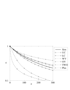
Figure 3: Learning curve for a GP with OU covariance function and inputs uniformly drawn from $x\in[0,1]^{d}$, at noise level $\sigma^{2}=0.05$. Left: $d=1$, length scale $l=0.01$. Right: $d=2$, $l=0.1$.

In Figure 3 we show the results for an OU covariance function with inputs from $[0,1]^{d}$, for $d=1$ (left) and $d=2$ (right). One observes that the lower bounds (Plaskota and OV) are rather loose in both cases. The TWO upper bound is also far from tight; the WV upper bound is better where it can be defined (for $d=1$). Our approximations, LC and UC, are closer to the true learning curve than any of the bounds and in fact appear to bracket it.

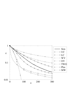
Figure 4: Learning curve for a GP with RBF covariance function and inputs uniformly drawn from $x\in[0,1]^{d}$, at noise level $\sigma^{2}=0.05$; dimension $d=1$, length scale $l=0.01$. We also show the MW bound here to show how it is first close to the Plaskota bound but then “misses” the change in behaviour where the generalization error crosses over into the asymptotic regime ($\epsilon\ll\sigma^{2}$).

Similar comments apply to Figure 4, which displays the results for an RBF covariance function with inputs from $[0,1]$. Because functions from an RBF prior are much smoother than those from an OU prior, they are easier to learn and the generalization error $\epsilon$ shows a more rapid decrease with $n$. This makes visible, within the range of $n$ shown, the anticipated change in behaviour as $\epsilon$ crosses over from the initial ($\epsilon\gg\sigma^{2}$) to the asymptotic ($\epsilon\ll\sigma^{2}$) regime. The LC approximation and, to a less quantitative extent, the Plaskota bound both capture this change. By contrast, the OV bound (as expected from its general properties discussed above) only shows the right qualitative behaviour in the asymptotic regime.

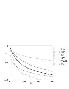
Figure 5: Learning curve for a GP with RBF covariance function and inputs uniformly drawn from $x\in[0,1]^{d}$, for dimension $d=4$ and length scale $l=0.3$. Left: noise level $\sigma^{2}=0.05$. Right: $\sigma^{2}=0.001$. Note that, for lower $\sigma^{2}$, the OV bound becomes looser as expected (it approaches zero for $\sigma^{2}\to 0$).

Figure 5 shows corresponding results in higher dimension ($d=4$), at two different noise levels $\sigma^{2}$. One observes in particular that the OV lower bound becomes looser as $\sigma^{2}$ decreases; this is as expected since for $\sigma^{2}\to 0$ the bound actually becomes void ($\epsilon_{\rm OV}\to 0$). The Plaskota bound also appears to get looser for lower $\sigma^{2}$, though not as dramatically. (Note that the kinks in the Plaskota curve are not an artifact: For larger $d$ the multiplicities of the different eigenvalues can be quite large; the value of $\epsilon_{\rm Pl}$ can become dominated by one such block of degenerate eigenvalues, and kinks occur where the dominant block changes.) The TWO upper bound, finally, is only weakly affected by the value of $\sigma^{2}$ and quite loose throughout.

Figure 6: Learning curve for a GP with RBF covariance function (length scale $l=0.01$) and inputs drawn from a Gaussian distribution in $d=1$ dimension; noise level $\sigma^{2}=0.05$. Note that the LC approximation provides less of a good representation of the overall shape of the learning curve here than for the previous examples with uniform input distributions. The curve labelled WV shows our generalized version of the Williams-Vivarelli bound (see eq. (23)).

Figure 7: Learning curve for a GP with RBF covariance function (length scale $l=0.3$) and inputs drawn from a Gaussian distribution in $d=4$ dimensions. Left: noise level $\sigma^{2}=0.05$. Right: $\sigma^{2}=0.001$. The OV lower bound is very loose for this smaller noise level. Note that, in contrast to all previous examples, there is a range of $n$ here where the true learning curve lies below the LC approximation.

All results shown so far pertain to uniform input distributions (over $[0,1]^{d}$). We now move to the last of our three scenarios, a GP with an RBF covariance function and inputs drawn from a Gaussian distribution (see App. C for details). In Figure 6 we see that in $d=1$ the (generalized) WV bound is still reasonably tight, while the LC approximation now provides less of a good representation of the overall shape of the learning curve than for the case of uniform input distributions. However, as in all previous examples, the LC and UC approximations still bracket the true learning curve (and come closer to it than the bounds). One is thus lead to speculate whether the approximations we have derived are actually bounds. Figure 7 shows this not to be the case, however: In $d=4$, the true learning curve drops visibly below the LC approximation in the small $n$ regime, and so the latter cannot be a lower bound. The low noise case ($\sigma^{2}=0.001$) shown here illustrates once more that the OV lower bound ceases to be useful for small noise levels.

In summary, of the approximations which we have derived, the LC approximation performs best. While we know on theoretical grounds that it will be accurate for large noise levels $\sigma^{2}$, the examples shown above demonstrate that it produces predictions close to the true learning curves even for the more realistic case of low noise levels (compared to the prior variance). As a general trend, agreement appears to be better for the case of uniform input distributions.

It is interesting at this stage to make a connection to the recent work of Malzahn and Opper Malzahn and Opper (2001). They devised an elegant way of approaching the learning curve problem from the point of view of statistical physics, calculating the relevant partition function (which is an average over data sets) using a so-called Gaussian variational approximation. The result they find for the Bayes error is identical to the LC approximation under the condition that $\epsilon(x)=\left\langle\epsilon(x,D)\right\rangle_{D}$, the $x$-dependent generalization error averaged over all data sets, is independent of $x$. Otherwise, they find a result of the same functional form, $\epsilon(n)={\rm tr\,}({\mathbf{\Lambda}}^{-1}+\eta{\mathbf{I}})^{-1}$, but the self-consistency equation for $\eta$ is more complicated than the simple relation $\eta=n/(\epsilon+\sigma^{2})$ obtained from the LC approximation (16). The LC approximation would thus be expected to perform less well for such “non-uniform” scenarios. This agrees qualitatively with our above findings: For the scenario with a Gaussian input distribution, the LC approximation is of poorer quality than for the cases with uniform input distributions over $[0,1]^{d}$.

4 Improving the approximations

In the previous section we saw that in our test scenarios the LC approximation (16) generally provides the closest theoretical approximation to the true learning curves. This may appear somewhat surprising, given that we made two rather drastic approximations in deriving (16): We treated the number of training examples $n$ as a continuous variable, and we decoupled the average of the right hand side of (10) into separate averages over numerator and denominator. We now investigate whether the LC prediction for the learning curves can be further improved by removing these approximations.

We begin with the effect of $n$, the number of training examples, taking only discrete (rather than continuous) values. Starting from (10), averaging numerator and denominator separately as before and introducing the auxiliary variable $v$ as in (13,14), we obtain

$$\epsilon(n+1)-\epsilon(n)=\frac{1}{\sigma^{2}+\epsilon}\frac{\partial\epsilon}{\partial v}$$ (25)

instead of (15). It is possible to interpolate between the two equations by writing

$$\frac{1}{\delta}[\epsilon(n+\delta)-\epsilon(n)]=\frac{1}{\sigma^{2}+\epsilon}\frac{\partial\epsilon}{\partial v}$$ (26)

Then $\delta=1$ corresponds to (25), which is the equation we wish to solve (discrete $n$), while in the limit $\delta\to 0$ we retrieve (15). To proceed, we treat $\delta$ as a perturbation parameter and assume that the solution of (26) can be expanded as

$$\epsilon=\epsilon_{0}+\delta\epsilon_{1}+{{\mathcal{O}}}(\delta^{2})$$

where $\epsilon_{0}\equiv\epsilon_{\rm LC}$. Expanding both sides of (26) to first order in $\delta$ yields

$$\frac{\partial\epsilon_{0}}{\partial n}+\delta\frac{\partial\epsilon_{1}}{\partial n}+\frac{1}{2}\delta\frac{\partial^{2}\epsilon_{0}}{\partial n^{2}}+{{\mathcal{O}}}(\delta^{2})=\left(\frac{1}{\sigma^{2}+\epsilon_{0}}-\delta\,\frac{\epsilon_{1}}{(\sigma^{2}+\epsilon_{0})^{2}}\right)\left(\frac{\partial\epsilon_{0}}{\partial v}+\delta\,\frac{\partial\epsilon_{1}}{\partial v}\right)$$

Comparing the coefficients of the ${{\mathcal{O}}}(\delta^{0})$ terms gives us back (15) for $\epsilon_{0}$, while from the ${{\mathcal{O}}}(\delta)$ terms we get

$$\frac{\partial\epsilon_{1}}{\partial n}-\frac{1}{\sigma^{2}+\epsilon_{0}}\frac{\partial\epsilon_{1}}{\partial v}=-\frac{1}{2}\frac{\partial^{2}\epsilon_{0}}{\partial n^{2}}-\frac{\epsilon_{1}}{(\sigma^{2}+\epsilon_{0})^{2}}\frac{\partial\epsilon_{0}}{\partial v}$$ (27)

This can again be solved using characteristics (see App. A), with the result

$$\epsilon_{1}=(\sigma^{2}+\epsilon_{0})\frac{n(a_{2}^{2}-a_{3})}{(1-na_{2})^{2}},\qquad a_{k}=(\sigma^{2}+\epsilon_{0})^{-k}\ {\rm tr\,}\left({\mathbf{\Lambda}}^{-1}+\frac{n}{\sigma^{2}+\epsilon_{0}}{\mathbf{I}}\right)^{-k}$$ (28)

Setting $\delta$ back to $1$ to have the case of discrete $n$ in (26), we then have

$$\epsilon_{\rm LC1}=\epsilon_{0}+\epsilon_{1}\equiv\epsilon_{\rm LC}+\epsilon_{1}$$

as the improved LC approximation that takes into account the effects of discrete $n$ (up to linear order in a perturbation expansion in $\delta$). We see that the correction term (28) is zero at $n=0$ as it must since $\epsilon_{\rm LC}$ gives the exact result $\epsilon={\rm tr\,}{\mathbf{\Lambda}}$ there. It can also be shown that $\epsilon_{1}<0$ for all nonzero $n$. This can be understood as follows: The decrease of $\epsilon(n)$ becomes smaller (in absolute value) as $n$ increases. Comparing (15) and (25), we see that the continuous $n$-approximation effectively averages the decrease term over the range $n\ldots n+1$ rather than evaluating it at $n$ itself; it therefore produces a smaller decrease in $\epsilon(n)$. The true decrease for discrete $n$ is larger, and so one expects the correction $\epsilon_{1}$ to be negative, in agreement with our calculation.

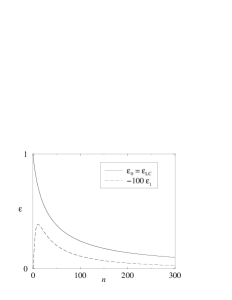
Figure 8: Solid line: LC approximation $\epsilon_{\rm LC}$ for the learning curve of a GP with RBF covariance function and Gaussian inputs. Parameters are as in Figure 7(left): Dimension $d=4$, length scale $l=0.3$, noise level $\sigma^{2}=0.05$. Dashed line: First order correction $\epsilon_{1}$ arising from the discrete nature of the number of training examples $n$. Note that $\epsilon_{1}$ has been multiplied by -100 to make it positive and visible on the scale of the values of $\epsilon_{\rm LC}$.

In Figure 8 we show $\epsilon_{\rm LC}$ and $\epsilon_{1}$ for one of the scenarios considered earlier; the results are typical also of what we find for other cases. The most striking observation is the smallness of $\epsilon_{1}$: Its absolute value is of the order of 1% of $\epsilon_{\rm LC}$ or less, and consequently $\epsilon_{\rm LC}$ and $\epsilon_{\rm LC1}$ are indistinguishable on the scale of the plot. On the one hand, this is encouraging: Given that $\epsilon_{1}$ is already so small, one would expect higher orders in a perturbation expansion in $\delta$ to yield even smaller corrections. Thus $\epsilon_{\rm LC1}$ is likely to be very close to the result that one would find if the discrete nature of $n$ was taken into account exactly. On the other hand, we also conclude that treating $n$ as discrete is not sufficient to turn the LC approximation into a lower bound on the learning curve; in Fig 6, for example, the curve for $\epsilon_{\rm LC1}$ would lie essentially on top of the one for $\epsilon_{\rm LC}$ and so still be significantly above the true learning curve for small $n$.

It is clear at this stage that in order to improve the LC approximation significantly one would have to address the decoupling of the numerator and denominator averages in (10). Generally, if $a$ and $b$ are random variables, one can evaluate the average of their ratio perturbatively as

$$\left\langle\frac{a}{b}\right\rangle=\left\langle\frac{\left\langle a\right\rangle+\Delta a}{\left\langle b\right\rangle+\Delta b}\right\rangle=\frac{\left\langle a\right\rangle}{\left\langle b\right\rangle}+\frac{\left\langle a\right\rangle}{\left\langle b\right\rangle^{3}}\left\langle(\Delta b)^{2}\right\rangle-\frac{1}{\left\langle b\right\rangle^{2}}\left\langle\Delta a\Delta b\right\rangle+\ldots$$

up to second order in the fluctuations. (This idea was used in Sollich (1994) to calculate finite $N$-corrections to the $N\to\infty$ limit of a linear learning problem.) To apply this to the average of the right hand side of (10) over the new training input $x_{n+1}$ and all previous ones, one would set

$$a={\mathcal{G}}(n)\mbox{\boldmath$\psi$}\mbox{\boldmath$\psi$}^{\mathrm{T}}{\mathcal{G}}(n),\qquad b=\sigma^{2}+\mbox{\boldmath$\psi$}^{\mathrm{T}}{\mathcal{G}}(n)\mbox{\boldmath$\psi$}$$

One then sees that averages such as $\left\langle ab\right\rangle$, required in $\left\langle\Delta a\Delta b\right\rangle=\left\langle ab\right\rangle-\left\langle a\right\rangle\left\langle b\right\rangle$, involve fourth-order averages $\left\langle\phi_{i}(x)\phi_{j}(x)\phi_{k}(x)\phi_{l}(x)\right\rangle_{x}$ of the components of $\psi$. In contrast to the second-order averages $\left\langle\phi_{i}(x)\phi_{j}(x)\right\rangle=\delta_{ij}$, such fourth-order statistics of the eigenfunctions do not have a simple, covariance function-independent form. Even if they were known, however, one would end up with averages over the entries of the matrix ${\mathcal{G}}$ which cannot be reduced to $\epsilon={\rm tr\,}\left\langle{\mathcal{G}}\right\rangle$ (e.g. by derivatives with respect to auxiliary parameters). Separate equations for the change of these averages with $n$ would then be required, generating new averages and eventually an infinite hierarchy which cannot be closed. We thus conclude that a perturbative approach is of little use in improving the LC approximation beyond the decoupling of averages. The approach of Malzahn and Opper (2001) thus looks more hopeful as far as the derivation of systematic corrections to the approximation is concerned.

5 How good can bounds and approximations be?

In this final section we ask whether there are limits of principle on the quality of theoretical predictions (either bounds or approximations) for GP learning curves. Of course this question is meaningless unless we specify what information the theoretical curves are allowed to exploit. Guided by the insight that all predictions discussed above depend (at least for uniform covariance functions) on the eigenvalues of the covariance function only (and of course the noise level $\sigma^{2}$), we ask: How tight can bounds and approximations be if they use only this eigenvalue spectrum as input?

To answer this question, it is useful to have a simple scenario with an arbitrary eigenvalue spectrum for which learning curves can be calculated exactly. Consider the case where the input space consists of $N$ discrete points $x^{\alpha}$; the input distribution is arbitrary, $P(x^{\alpha})=p_{\alpha}$ with $\sum_{\alpha}p_{\alpha}=1$. Take the covariance function to be degenerate in the sense that there are no correlations between different points: $C(x^{\alpha},x^{\beta})=c_{\alpha}\delta_{\alpha\beta}$. The eigenvalue equation (6) then becomes simply

$$\sum_{\beta}C(x^{\alpha},x^{\beta})\phi(x^{\beta})p_{\beta}=c_{\alpha}p_{\alpha}\phi(x^{\alpha})=\lambda\phi(x^{\alpha})$$

so that the $N$ different eigenvalues are $\lambda_{\alpha}=c_{\alpha}p_{\alpha}$. The eigenfunctions are $\phi_{\alpha}(x^{\beta})=p_{\alpha}^{-1/2}\delta_{\alpha\beta}$, where the prefactor follows from the normalization condition $\sum_{\gamma}p_{\gamma}\phi_{\alpha}(x^{\gamma})\phi_{\beta}(x^{\gamma})=\delta_{\alpha\beta}$. Note that by choosing the $c_{\alpha}$ and $p_{\alpha}$ appropriately, the $\lambda_{\alpha}$ can be adjusted to any desired value in this setup. The same still holds even if we require the covariance function to be uniform, i.e., $c_{\alpha}$ to be independent of $\alpha$.

A set of $n$ training inputs is, in this scenario, fully characterized by how often it contains each of the possible inputs $x^{\alpha}$; we call these numbers $n_{\alpha}$. The generalization error is easy to work out from (8), using

$$({\mathbf{\Psi}}^{\mathrm{T}}{\mathbf{\Psi}})_{\alpha\beta}=\sum_{\gamma}n_{\gamma}\phi_{\alpha}(x^{\gamma})\phi_{\beta}(x^{\gamma})=(n_{\alpha}/p_{\alpha})\delta_{\alpha\beta}.$$

This shows that ${\mathbf{\Psi}}^{\mathrm{T}}{\mathbf{\Psi}}$ is a diagonal matrix, and thus from (8)

$$\epsilon(D)={\rm tr\,}({\mathbf{\Lambda}}^{-1}+\sigma^{-2}{\mathbf{\Psi}}^{\mathrm{T}}{\mathbf{\Psi}})^{-1}=\sum_{\alpha}\left(\lambda_{\alpha}^{-1}+\sigma^{-2}n_{\alpha}/p_{\alpha}\right)^{-1}=\sum_{\alpha}\lambda_{\alpha}\frac{\sigma^{2}}{\sigma^{2}+n_{\alpha}\lambda_{\alpha}/p_{\alpha}}$$ (29)

This has the expected form: The contribution of each eigenvalue is reduced according to the ratio of the noise level $\sigma^{2}$ and the signal $n_{\alpha}\lambda_{\alpha}/p_{\alpha}=n_{\alpha}c_{\alpha}$ received at the corresponding input point. To average this over all training sets of size $n$, one notices that $n_{\alpha}$ has a binomial distribution, so that

$$\epsilon(n)=\sum_{\alpha}\lambda_{\alpha}\sum_{n_{\alpha}=0}^{n}\left(\!\!\begin{array}[]{c}n\\ n_{\alpha}\end{array}\!\!\right)p_{\alpha}^{n_{\alpha}}(1-p_{\alpha})^{n-n_{\alpha}}\frac{\sigma^{2}}{\sigma^{2}+n_{\alpha}\lambda_{\alpha}/p_{\alpha}}$$

Writing $(\sigma^{2}+n_{\alpha}\lambda_{\alpha}/p_{\alpha})^{-1}=\sigma^{-2}\int_{0}^{1}\!dr\ r^{n_{\alpha}\lambda_{\alpha}/p_{\alpha}\sigma^{2}}$, we can perform the sum over $n_{\alpha}$ and obtain

$$\epsilon(n)=\int_{0}^{1}\!dr\ \sum_{\alpha}\lambda_{\alpha}\left(1-p_{\alpha}+p_{\alpha}r^{\lambda_{\alpha}/p_{\alpha}\sigma^{2}}\right)^{n}$$ (30)

as the final result; the integral over $r$ can easily be performed numerically for given set of eigenvalues $\lambda_{\alpha}$ and input probabilities $p_{\alpha}$. Note that, having done the calculation for a finite number $N$ of discrete inputs points (and therefore of eigenvalues), we can now also take $N$ to infinity and therefore analyse scenarios (such as the ones studied in Sec. 3) with an infinite number of nonzero eigenvalues.

A simple limiting case will now tell us about the quality of eigenvalue-dependent upper bounds on learning curves. Assume that one of the $p_{\alpha}$ is close to $1$, whereas all the other ones are close to $0$. From (30), one then sees that only the contribution from the eigenvalue $\lambda_{\alpha}$ with $p_{\alpha}\approx 1$ is reduced as $n$ increases while all other ones remain unaffected, so that

$$\epsilon(n)\approx{\rm tr\,}{\mathbf{\Lambda}}-\lambda_{\alpha}+\frac{\lambda_{\alpha}\sigma^{2}}{\sigma^{2}+n\lambda_{\alpha}}={\rm tr\,}{\mathbf{\Lambda}}-\frac{n\lambda_{\alpha}^{2}}{\sigma^{2}+n\lambda_{\alpha}}\geq{\rm tr\,}{\mathbf{\Lambda}}-\lambda_{\alpha}$$ (31)

If $\lambda_{\alpha}\ll{\rm tr\,}{\mathbf{\Lambda}}$, then we can make the reduction in generalization error arbitrarily small. It thus follows that there is no non-trivial upper bound on learning curves that takes only the eigenvalue spectrum of the covariance function as input. [Accordingly, the two non-asymptotic upper bounds (WV and TWO) discussed in Sec. 3 both contain other information, via the weighted averages of $C_{s}^{2}(x)=C^{2}(0,x)$ in (21) and the average of $C(x,x)\phi_{i}^{2}(x)$ in (24).] In particular, this implies that our UC approximation cannot be an upper bound (even though the results for all scenarios investigated above suggested that it might be). Furthermore, our result shows that lower bounds on the generalization error (e.g. the OV or Plaskota bounds) can be arbitrarily loose. A similar observation holds for upper bounds on the (data set-averaged) training error $\epsilon_{\rm t}$: Opper and Vivarelli showed Opper and Vivarelli (1999) that their $\epsilon_{\rm OV}$ actually also provides an upper bound for this quantity (so that the two errors ‘sandwich’ the bound, $\epsilon_{\rm t}\leq\epsilon_{\rm OV}\leq\epsilon$). In the present case it is easy to calculate $\epsilon_{\rm t}$ explicitly; we omit details and just quote the result

$$\epsilon_{\rm t}\approx\frac{\lambda_{\alpha}\sigma^{2}}{\sigma^{2}+n\lambda_{\alpha}}\leq\lambda_{\alpha}$$

By taking $\lambda_{\alpha}\ll{\rm tr\,}{\mathbf{\Lambda}}$, one then sees that the upper bound $\epsilon_{\rm OV}$ can be made arbitrarily loose for any fixed $n$ (and that the ratio of training and generalization error can be made arbitrarily small).

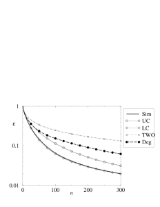
Figure 9: Learning curve for a GP with RBF covariance function and inputs uniformly drawn from $x\in[0,1]^{d}$. Parameters are as in Figure 5(left): Dimension $d=4$, length scale $l=0.3$ and noise level $\sigma^{2}=0.05$. The curves Sim (true learning curve, from numerical simulations), UC, LC and TWO are also as in Figure 5(left). The curve labelled “Deg” shows the exact learning curve for the degenerate scenario (outputs for different inputs are uncorrelated) with exactly the same spectrum of eigenvalues $\lambda_{i}$ of the covariance function (and uniform prior variance $C(x,x)$). The curves Sim and Deg differ significantly, showing that learning curves cannot be predicted reliably based on eigenvalues alone.

One may object that the above limit of most of the $p_{\alpha}$ tending to zero is unrealistic because it implies that the corresponding prior variances $c_{\alpha}=\lambda_{\alpha}/p_{\alpha}$ would become very large. Let us therefore now restrict the prior variance to be uniform, $c_{\alpha}=c$. It then follows that $\lambda_{\alpha}=c/p_{\alpha}$ and hence $p_{\alpha}=\lambda_{\alpha}/{\rm tr\,}{\mathbf{\Lambda}}$. With this assumption, only the $\lambda_{\alpha}$ and $\sigma^{2}$ remain as parameters affecting the learning curve (30). The results for an eigenvalue spectrum from one of the situations covered in Sec. 3 are shown in Figure 9. The main conclusion to be drawn is that the learning curves for the present scenario are quite different from the ones we found earlier, even though the eigenvalue spectra and noise levels are, by construction, precisely identical. This demonstrates that theoretical predictions for learning curves which only take into account the eigenvalue spectrum of a covariance function cannot universally match the true learning curves with a high degree of accuracy; the quality of approximation will vary depending on details of the covariance function and input distribution that are not encoded in the spectrum. Note that Figure 9 also provides a concrete example for the fact that the UC approximation is not in general an upper bound on the true learning curve; in fact, it here underestimates the true $\epsilon(n)$ quite significantly.

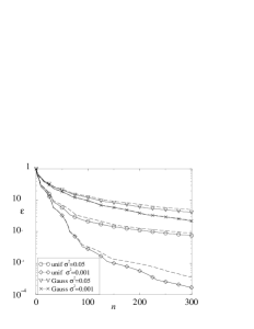
Figure 10: Comparison of the Plaskota bound (solid lines) and the lowest generalization error achievable for single data sets of size $n$ within the degenerate scenario (dashed lines). The eigenvalue spectra used to construct the curves are those for an RBF covariance function with length scale $l=0.3$, in $d=4$ dimensions, and for the input distributions (uniform over $[0,1]^{d}$, or Gaussian) shown in the legend; the noise level $\sigma^{2}$ is also given there. Note that for a given $n$, the curves become closer for lower $\sigma^{2}$; this is as expected since for $\sigma^{2}\to 0$ the Plaskota bound can be saturated for a specific data set (see text).

We can also use the present scenario to assess whether, as a bound on the generalization error resulting from a single training set, the Plaskota bound (19) could be significantly improved. We focus on the case of uniform covariance functions, where (29) becomes

$$\epsilon(D)=\sum_{\alpha}\lambda_{\alpha}\frac{\sigma^{2}}{\sigma^{2}+n_{\alpha}{\rm tr\,}{\mathbf{\Lambda}}}$$ (32)

For any assignment of the $n_{\alpha}$ there is at least one training set of size $n=\sum_{\alpha}n_{\alpha}$ for which the generalization error is given by (32). Minimizing numerically over the $n_{\alpha}$ for each given $n$, we find the curves shown in Figure 10, where the Plaskota bounds for the same eigenvalue spectra are also shown. The curves are quite close to each other, implying that the Plaskota bound cannot be significantly tightened as a single data set bound (assuming, as throughout, that the improved bound would again only be based on the covariance function’s eigenvalue spectrum). In the limit $\sigma^{2}\to 0$, the bound—which then reduces to the MW bound  (18)—cannot be tightened at all, as setting $n_{\alpha}=1$ for $\alpha=1\ldots n$ and $n_{\alpha}=0$ for $\alpha\geq n+1$ in (32) shows.

Within the simple degenerate scenario introduced in this section, we finally comment briefly on a universal relation recently proposed by Malzahn and Opper Malzahn and Opper (2001). They suggest considering an empirical estimate of the (Bayes) generalization error, which is obtained by replacing the average over all inputs $x$ by one over the $n$ training inputs $x_{i}$:

$$\epsilon_{\rm emp}(D)=\frac{1}{n}\sum_{i=1}^{n}\epsilon(x_{i},D)$$

Within the approximations of their calculation, the data set average of this quantity is then universally linked to a modified version of the true generalization error:

$$\left\langle\epsilon_{\rm emp}(D)\right\rangle_{D}=\left\langle\frac{\epsilon(x)}{\sigma^{2}+\epsilon(x)}\right\rangle_{x}$$ (33)

Note that the average over data sets is on the ‘inside’ of the fraction on the right hand side, through the definition of $\epsilon(x)=\left\langle\epsilon(x,D)\right\rangle_{D}$. Within our degenerate scenario, we can calculate both sides of (33) explicitly, but find no obvious relation between the two sides. However, if we move the data set average on the right hand side to the outside, we do (after a brief calculation, the details of which we omit) find a simple result:

$$\left\langle\epsilon_{\rm emp}(D_{n+1})\right\rangle_{D_{n+1}}=\left\langle\left\langle\frac{\epsilon(x,D_{n})}{\sigma^{2}+\epsilon(x,D_{n})}\right\rangle_{\!\!x}\,\right\rangle_{\!\!D_{n}}$$ (34)

As indicated by the subscripts, the left hand side of this relation is to be evaluated for data sets of size $n+1$ rather than $n$. The result (34) is remarkable in that it holds for any eigenvalue spectrum and any input distribution (within the degenerate scenario considered here). We take this as a hopeful sign that some universal link between true and empirical generalization errors, along the lines derived by Malzahn and Opper (2001) within their approximation, may indeed exist.

6 Conclusion

In summary, we have derived an exact representation of the average generalization $\epsilon$ error of Gaussian processes used for regression, in terms of the eigenvalue decomposition of the covariance function. Starting from this, we obtained two different approximations (LC and UC) to the learning curve $\epsilon(n)$. Both become exact in the large noise limit; in practice, one generically expects the opposite case ($\sigma^{2}/C(x,x)\ll 1$), but comparison with simulation results shows that even in this regime the new approximations perform well.

The LC approximation in particular represents the overall shape of the learning curves very well, both for ‘rough’ (OU) and ‘smooth’ (RBF) Gaussian priors, and for small as well as for large numbers of training examples $n$. It is not perfect, but does generally get substantially closer to the true learning curves than existing bounds (two of which, due to Plaskota and to Williams and Vivarelli, we generalized to a wider range of scenarios). For situations with non-uniform input distributions the predictions of the LC approximation tend to be less accurate, and we linked this observation to recent work by Malzahn and Opper Malzahn and Opper (2001) on the effects of non-uniformity across input space. Their result, which reduces to the LC approximation for sufficiently uniform scenarios, may in other cases provide better approximations, but this has to be traded off against the higher computational cost that would be involved in actually evaluating the predictions.

We then discussed how the LC approximation could be improved. The effects of discrete $n$ can be incorporated to leading order, but were seen to be relatively minor; on the other hand, the second approximation involved in the derivation (decoupling of averages) appears difficult to improve on within our framework.

Finally, we investigated a simple “degenerate” Gaussian process learning scenario, where the outputs corresponding to different inputs are uncorrelated. This provided us with a means of assessing whether there are limits on the quality of approximations and bounds that take into account only the eigenvalue spectrum of the covariance function. We found indeed that such limits exist: There can be no nontrivial upper bound on the learning curve of this form, and approximations are necessarily of limited quality because different covariance functions with the same eigenvalue spectrum can produce rather different learning curves. We also found that as a bound on the generalization error for single data sets (rather than its average over data sets) the Plaskota bound is close to being tight. Whether a tight lower bound on the average learning curve exists remains an open question; one plausible candidate worth investigating would be the average generalization error of our degenerate scenario, minimized over all possible input distributions for a fixed eigenvalue spectrum.

There are a number of open problems. One is whether a sub-class of GP learning scenarios can be defined for which the covariance function’s eigenvalue spectrum is sufficient to predict the learning curves accurately. Alternatively, one could ask what (minimal) extra information beyond the eigenvalue spectrum needs to be taken into account to arrive at accurate learning curves for all possible GP regression problems. Finally, one may wonder whether the eigenvalue decomposition we have chosen, which explicitly depends on the input distribution, is really the optimal one. On the one hand, recent work (see e.g. Williams and Seeger (2000)) appears to answer this question in the affirmative. On the other hand, the variability of learning curves among GP covariance functions with the same eigenvalue spectrum suggests that the eigenvalues alone do not provide sufficient information for accurate predictions. One may therefore speculate that eigendecompositions with respect to other input distributions (e.g., maximum entropy ones) might not suffer from this problem. We leave these challenges for future work.

Acknowledgements: We would like to thank Chris Williams, Manfred Opper and Dörte Malzahn for stimulating discussions, and the Royal Society for financial support through a Dorothy Hodgkin Research Fellowship.

Appendix A Solving for the LC approximation

In this appendix we describe how to solve eqns. (15,27) for the LC approximation and its first order correction, using the method of characteristic curves. The method applies to partial differential equations of the form $a\,\partial f/\partial x+b\,\partial f/\partial y=c$, where $f=f(x,y)$ and $a,b,c$ can be arbitrary functions of $x,y,f$. Viewing the solution as a surface in $x,y,f$-space, one can then show John (1978) that if the point $(x_{0},y_{0},f_{0})$ belongs to the solution surface then so does the entire characteristic curve $(x(t),y(t),f(t))$ defined by

$$\frac{dx}{dt}=a,\qquad\frac{dy}{dt}=b,\qquad\frac{df}{dt}=c,\qquad(x(0),y(0),f(0))=(x_{0},y_{0},f_{0})$$

The solution surface can then be recovered by combining an appropriate one-dimensional family of characteristic curves.

Denote the generalization error predicted by the LC approximation as $\epsilon_{0}(n,v)$, with $v$ the auxiliary parameter introduced in (13,14). It is the solution of the equation (15)

$$\frac{\partial\epsilon_{0}}{\partial n}-\frac{1}{\sigma^{2}+\epsilon_{0}}\frac{\partial\epsilon_{0}}{\partial v}=0$$

subject to the initial conditions $\epsilon_{0}(n=0,v)={\rm tr\,}({\mathbf{\Lambda}}^{-1}+v{\mathbf{I}})^{-1}$. These give us a family of solution points which the characteristic curves have to pass through, namely $(n(0)=0,v(0)=v_{0},\epsilon_{0}(0)={\rm tr\,}({\mathbf{\Lambda}}^{-1}+v_{0}{\mathbf{I}})^{-1})$. The equations for the characteristic curves are

$$\frac{dn}{dt}=1,\qquad\frac{dv}{dt}=-\frac{1}{\sigma^{2}+\epsilon_{0}},\qquad\frac{d\epsilon_{0}}{dt}=0$$

and can be integrated to give

$$n=n(0)+t=t,\qquad v=v(0)-\frac{t}{\sigma^{2}+\epsilon_{0}}=v_{0}-\frac{t}{\sigma^{2}+\epsilon_{0}},\qquad\epsilon_{0}=\epsilon_{0}(0)={\rm tr\,}({\mathbf{\Lambda}}^{-1}+v_{0}{\mathbf{I}})^{-1}$$ (35)

Eliminating $t$ (the curve parameter) and $v_{0}$ (which parameterizes the family of initial points) gives the required solution $\epsilon_{0}={\rm tr\,}\{{\mathbf{\Lambda}}^{-1}+[v+n/(\sigma^{2}+\epsilon_{0})]{\mathbf{I}}\}^{-1}$. The LC approximation (16) is obtained by setting $v=0$.

For the first order correction $\epsilon_{1}$, we have to solve the equation (27)

$$\frac{\partial\epsilon_{1}}{\partial n}-\frac{1}{\sigma^{2}+\epsilon_{0}}\frac{\partial\epsilon_{1}}{\partial v}=-\frac{1}{2}\frac{\partial^{2}\epsilon_{0}}{\partial n^{2}}-\frac{\epsilon_{1}}{(\sigma^{2}+\epsilon_{0})^{2}}\frac{\partial\epsilon_{0}}{\partial v}$$

with the initial condition (explained in the main text) $\epsilon_{1}(n=0,v)=0$. Hence a suitable family of initial solution points is $(n(0)=0,v(0)=v_{0},\epsilon_{1}(0)=0)$. The characteristic curves must obey

$$\frac{dn}{dt}=0,\qquad\frac{dv}{dt}=-\frac{1}{\sigma^{2}+\epsilon_{0}},\qquad\frac{d\epsilon_{1}}{dt}=-\frac{1}{2}\frac{\partial^{2}\epsilon_{0}}{\partial n^{2}}-\frac{\epsilon_{1}}{(\sigma^{2}+\epsilon_{0})^{2}}\frac{\partial\epsilon_{0}}{\partial v}$$

The solutions for the $n(t)$ and $v(t)$-dependence are therefore the same as before, and as a result $\epsilon_{0}$ is again constant along the characteristic curves. For the derivatives of $\epsilon_{0}$ that appear, one finds after some algebra

$$\frac{\partial\epsilon_{0}}{\partial v}=-(\sigma^{2}+\epsilon_{0})^{2}\frac{a_{2}}{1-na_{2}},\qquad\frac{\partial^{2}\epsilon_{0}}{\partial n^{2}}=-2(\sigma^{2}+\epsilon_{0})\frac{a_{2}^{2}-a_{3}}{(1-na_{2})^{3}}$$

Here we have used the definitions from (28); because both $a_{2}$ and $a_{3}$ only depend on $n$ and $v$ in the combination $v+n/(\sigma^{2}+\epsilon_{0})$, they are also constant along the characteristic curves. Using also that $n=t$ from (35), the equation for $\epsilon_{1}$ becomes

$$\frac{d\epsilon_{1}}{dt}=(\sigma^{2}+\epsilon_{0})\frac{a_{2}^{2}-a_{3}}{(1-ta_{2})^{3}}+\epsilon_{1}\frac{a_{2}}{1-ta_{2}}$$

This linear differential equation is easily integrated; using the initial condition $\epsilon_{1}(0)=0$ one finds

$$\epsilon_{1}=(\sigma^{2}+\epsilon_{0})\frac{t(a_{2}^{2}-a_{3})}{(1-ta_{2})^{2}}$$

Eliminating $t$ again via $t=n$ finally gives the solution (28).

Appendix B The Plaskota bound and its extension

To summarize the proof of Plaskota’s lower bound on learning curves Plaskota (1990) and generalize it to non-uniform covariance functions, we find it most convenient to work with a discrete space of inputs $x^{\alpha}$, $\alpha=1\ldots N$, with input probabilities $P(x^{\alpha})=p_{\alpha}$. (The case where inputs can vary continuously can be approximated arbitrarily well by such a scenario, either by discretizing the input space on a sufficiently fine grid or by taking the $x^{\alpha}$ as a large number $N$ of samples from the input distribution and setting $p_{\alpha}=1/N$.) A function $\theta$ on these inputs can then be thought of as a vector $\theta$ with elements $\theta(x^{\alpha})$; similarly, the covariance function $C(x^{\alpha},x^{\beta})\equiv C_{\alpha\beta}$ becomes an $N\times N$ matrix ${\mathbf{C}}=\left\langle\mbox{\boldmath$\theta$}\mbox{\boldmath$\theta$}^{\mathrm{T}}\right\rangle$. The eigenvalue equation (6) and the corresponding normalization condition then read

$$\sum_{\beta}C_{\alpha\beta}p_{\beta}\phi_{i}(x^{\beta})=\lambda_{i}\phi_{i}(x^{\alpha}),\qquad\sum_{\alpha}\phi_{i}(x^{\alpha})\phi_{j}(x^{\alpha})p_{\alpha}=\delta_{ij}$$

We can write these in a more compact form: If we set ${\mathbf{\Lambda}}=\mbox{diag}(\lambda_{1}\ldots\lambda_{N})$ and ${\mathbf{P}}=\mbox{diag}(p_{1}\ldots p_{N})$, denote $\mbox{\boldmath$\phi$}_{i}$ the vector with entries $\phi_{i}(x^{\alpha})$ and ${\mathbf{\Phi}}$ the $N\times N$ matrix whose columns are the $\mbox{\boldmath$\phi$}_{i}$, we have

$${\mathbf{C}}{\mathbf{P}}{\mathbf{\Phi}}={\mathbf{\Phi}}{\mathbf{\Lambda}},\qquad{\mathbf{\Phi}}^{\mathrm{T}}{\mathbf{P}}{\mathbf{\Phi}}={\mathbf{I}}$$

and hence

$${\mathbf{C}}={\mathbf{\Phi}}{\mathbf{\Lambda}}{\mathbf{\Phi}}^{\mathrm{T}}$$

One can also write this in the form of a more conventional matrix diagonalization:

$${\mathbf{P}}^{1/2}{\mathbf{C}}{\mathbf{P}}^{1/2}=({\mathbf{P}}^{1/2}{\mathbf{\Phi}}){\mathbf{\Lambda}}({\mathbf{P}}^{1/2}{\mathbf{\Phi}})^{\mathrm{T}},\qquad({\mathbf{P}}^{1/2}{\mathbf{\Phi}})^{\mathrm{T}}({\mathbf{P}}^{1/2}{\mathbf{\Phi}})={\mathbf{I}}$$

It follows that the $\lambda_{i}$ are the eigenvalues of the matrix ${\mathbf{P}}^{1/2}{\mathbf{C}}{\mathbf{P}}^{1/2}$ and that

$$\left\langle C(x,x)\right\rangle_{x}\equiv{\rm tr\,}{\mathbf{P}}{\mathbf{C}}={\rm tr\,}{\mathbf{P}}^{1/2}{\mathbf{C}}{\mathbf{P}}^{1/2}={\rm tr\,}{\mathbf{\Lambda}}$$ (36)

in agreement with (7).

Plaskota now considers the case of generalized training sets consisting of $n$ generalized observations $y_{l}={\mathbf{L}}_{l}^{\mathrm{T}}\mbox{\boldmath$\theta$}+\eta_{l}$. Each $y_{l}$ is a linear combinations of the values of the function $\theta(x)$, with coefficients specified by the vector ${\mathbf{L}}_{l}$, corrupted by additive Gaussian noise $\eta_{l}$ which as before we take to be of variance $\sigma^{2}$. The conventional scenario, where each training point contains a (corrupted) observation of $\theta(x)$ at a single point $x=x^{\alpha(l)}$, corresponds to ${\mathbf{L}}_{l}={\mathbf{e}}_{\alpha(l)}$. Here we denote ${\mathbf{e}}_{\alpha}$ the $\alpha$-th unit vector (with the $\alpha$-th component equal to one and all others zero) and write the $l$-th training input as $x^{\alpha(l)}$, with $\alpha(l)\in\{1\ldots N\}$.

After the observation of the $y_{l}$, we will have some posterior covariances $\left\langle\Delta\theta(x^{\alpha})\Delta\theta(x^{\beta})\right\rangle$. Collecting these into an $N\times N$ matrix ${\mathbf{V}}$ one can write them explicitly as

$${\mathbf{V}}={\mathbf{C}}-{\mathbf{C}}{\mathbf{L}}({\mathbf{L}}^{\mathrm{T}}{\mathbf{C}}{\mathbf{L}}+\sigma^{2}{\mathbf{I}})^{-1}{\mathbf{L}}^{\mathrm{T}}{\mathbf{C}}=({\mathbf{C}}^{-1}+\sigma^{-2}{\mathbf{L}}{\mathbf{L}}^{\mathrm{T}})^{-1}$$ (37)

where ${\mathbf{L}}$ is an $N\times n$ matrix whose columns are the ${\mathbf{L}}_{l}$. The first version of this result can be seen as a generalization of (2); the second version is the corresponding generalization of (8) in a different guise. It then follows that the generalization error is given by

$$\epsilon(D)=\sum_{\alpha}p_{\alpha}\left\langle(\Delta\theta(x^{\alpha}))^{2}\right\rangle={\rm tr\,}{\mathbf{P}}{\mathbf{V}}={\rm tr\,}{\mathbf{P}}{\mathbf{C}}-{\rm tr\,}[{\mathbf{L}}^{\mathrm{T}}{\mathbf{C}}{\mathbf{P}}{\mathbf{C}}{\mathbf{L}}({\mathbf{M}}+\sigma^{2}{\mathbf{I}})^{-1}]$$ (38)

where we have defined the $n\times n$ matrix ${\mathbf{M}}={\mathbf{L}}^{\mathrm{T}}{\mathbf{C}}{\mathbf{L}}$. Its trace (which will become important shortly) is ${\rm tr\,}{\mathbf{M}}=\sum_{l}{\mathbf{L}}_{l}{\mathbf{C}}{\mathbf{L}}_{l}$; for a conventional training set with training inputs $x^{\alpha(l)}$ this becomes ${\rm tr\,}{\mathbf{M}}=\sum_{l}{\mathbf{e}}_{\alpha(l)}^{\mathrm{T}}{\mathbf{C}}{\mathbf{e}}_{\alpha(l)}=\sum_{l}C(x^{\alpha(l)},x^{\alpha(l)})$.

So far everything is exact. The idea behind Plaskota’s bound is now as follows: For any given conventional training set with $n$ training inputs, minimize $\epsilon(D)$ over all generalized training sets of size $n$ which have the same value of ${\rm tr\,}{\mathbf{M}}$. The result then clearly gives a lower bound on $\epsilon(D)$ for the given training set.

To carry out this minimization, one can proceed as follows. The matrix ${\mathbf{M}}$ is symmetric and can be diagonalized, so that ${\mathbf{M}}={\mathbf{O}}\mbox{\boldmath$\eta$}{\mathbf{O}}^{\mathrm{T}}$ where ${\mathbf{O}}$ is an orthogonal $n\times n$ matrix and $\eta$ is a diagonal matrix whose entries $\eta_{i}$ are the eigenvalues of ${\mathbf{M}}$. Since ${\mathbf{M}}$ is positive semi-definite, the $\eta_{i}$ are non-negative; we also assume them to be ordered in descending order, $\eta_{1}\geq\ldots\geq\eta_{N}$. It then follows that $({\mathbf{M}}+\sigma^{2}{\mathbf{I}})^{-1}={\mathbf{O}}(\mbox{\boldmath$\eta$}+\sigma^{2}{\mathbf{I}})^{-1}{\mathbf{O}}^{\mathrm{T}}$, so that

$$\epsilon(D)={\rm tr\,}{\mathbf{\Lambda}}-{\rm tr\,}[{\mathbf{O}}^{\mathrm{T}}{\mathbf{L}}^{\mathrm{T}}{\mathbf{C}}{\mathbf{P}}{\mathbf{C}}{\mathbf{L}}{\mathbf{O}}(\mbox{\boldmath$\eta$}+\sigma^{2}{\mathbf{I}})^{-1}]$$

where we have also used that ${\rm tr\,}{\mathbf{P}}{\mathbf{C}}={\rm tr\,}{\mathbf{\Lambda}}$ from (36). Now, if we define the $N\times n$ matrix ${\mathbf{Q}}={\mathbf{C}}^{1/2}{\mathbf{L}}{\mathbf{O}}\mbox{\boldmath$\eta$}^{-1/2}$ and write ${\mathbf{\tilde{C}}}={\mathbf{C}}^{1/2}{\mathbf{P}}{\mathbf{C}}^{1/2}$, then $\mbox{\boldmath$\eta$}^{1/2}{\mathbf{Q}}^{\mathrm{T}}{\mathbf{\tilde{C}}}{\mathbf{Q}}\mbox{\boldmath$\eta$}^{1/2}={\mathbf{O}}^{\mathrm{T}}{\mathbf{L}}^{\mathrm{T}}{\mathbf{C}}{\mathbf{P}}{\mathbf{C}}{\mathbf{L}}{\mathbf{O}}$ and so

$$\epsilon(D)={\rm tr\,}{\mathbf{\Lambda}}-{\rm tr\,}[{\mathbf{Q}}^{\mathrm{T}}{\mathbf{\tilde{C}}}{\mathbf{Q}}\mbox{\boldmath$\eta$}(\mbox{\boldmath$\eta$}+\sigma^{2}{\mathbf{I}})^{-1}]={\rm tr\,}{\mathbf{\Lambda}}-\sum_{i=1}^{n}({\mathbf{Q}}^{\mathrm{T}}{\mathbf{\tilde{C}}}{\mathbf{Q}})_{ii}\frac{\eta_{i}}{\eta_{i}+\sigma^{2}}$$ (39)

To minimize $\epsilon(D)$, we need to make the sum over $i$ maximal. If we write the $n$ columns of ${\mathbf{Q}}$ as vectors ${\mathbf{Q}}_{i}$ then $({\mathbf{Q}}^{\mathrm{T}}{\mathbf{\tilde{C}}}{\mathbf{Q}})_{ii}={\mathbf{Q}}_{i}^{\mathrm{T}}{\mathbf{\tilde{C}}}{\mathbf{Q}}_{i}$; also, from the definition of ${\mathbf{Q}}$ we have ${\mathbf{Q}}^{\mathrm{T}}{\mathbf{Q}}={\mathbf{I}}$, implying that the ${\mathbf{Q}}_{i}$ are orthonormal. Now it is easy to see that ${\mathbf{\tilde{C}}}={\mathbf{C}}^{1/2}{\mathbf{P}}{\mathbf{C}}^{1/2}$ has the same eigenvalues as ${\mathbf{P}}^{1/2}{\mathbf{C}}{\mathbf{P}}^{1/2}$, namely, the $\lambda_{i}$. Assuming these to be ordered in a descending sequence, the largest value that ${\mathbf{Q}}_{i}^{\mathrm{T}}{\mathbf{\tilde{C}}}{\mathbf{Q}}_{i}$ can take is therefore $\lambda_{1}$. Because of the orthonormality of the ${\mathbf{Q}}_{i}$, one has similarly that $\sum_{i\leq k}{\mathbf{Q}}_{i}^{\mathrm{T}}{\mathbf{\tilde{C}}}{\mathbf{Q}}_{i}\leq\sum_{i\leq k}\lambda_{i}$ for all $k\leq n$. Since the terms $\eta_{i}/(\eta_{i}+\sigma^{2})$ form a descending sequence (due to our assumed ordering of the $\eta_{i}$), it is then clear that the optimal situation is the one where ${\mathbf{Q}}_{1}^{\mathrm{T}}{\mathbf{\tilde{C}}}{\mathbf{Q}}_{1}$, multiplying the largest value $\eta_{1}/(\eta_{1}+\sigma^{2})$, has the largest possible value $\lambda_{1}$, ${\mathbf{Q}}_{2}^{\mathrm{T}}{\mathbf{\tilde{C}}}{\mathbf{Q}}_{2}$ has the largest possible value subject to this, which is $\lambda_{2}$, and so on. Plaskota indeed proved formally that

$$\epsilon(D)\geq{\rm tr\,}{\mathbf{\Lambda}}-\sum_{i=1}^{n}\frac{\lambda_{i}\eta_{i}}{\eta_{i}+\sigma^{2}}$$

Finally, one can now optimize over the $\eta_{i}$, subject to the constraint that we imposed initially, i.e., that ${\rm tr\,}{\mathbf{M}}=\sum_{i}\eta_{i}$ equals the sum $S=\sum_{l}C(x^{\alpha(l)},x^{\alpha(l)})$. This gives the final Plaskota bound

$$\epsilon(D)\geq{\rm tr\,}{\mathbf{\Lambda}}-\max_{\{\eta_{i}\}}\sum_{i=1}^{n}\frac{\lambda_{i}\eta_{i}}{\eta_{i}+\sigma^{2}}=\min_{\{\eta_{i}\}}\left(\sum_{i=1}^{n}\frac{\lambda_{i}\sigma^{2}}{\eta_{i}+\sigma^{2}}\right)+\sum_{i\geq n+1}\lambda_{i}$$ (40)

as given in (19). Plaskota also proved this bound to be realizable by an appropriate choice of the generalized observations ${\mathbf{L}}_{l}$. His original derivation only applied to uniform covariance functions, but the above proof sketch shows that this restriction is not in fact necessary.

To evaluate the Plaskota bound in practice it is desirable to have a more explicit expression for the minimum over the $\eta_{i}$. Introducing a Lagrange multiplier $\alpha$ for the constraint $\sum_{i}\eta_{i}=S$, one finds by differentiation of (40) that each positive $\eta_{i}$ must satisfy

$$-\frac{\lambda_{i}\sigma^{2}}{(\eta_{i}+\sigma^{2})^{2}}+\alpha=0$$ (41)

while for the vanishing $\eta_{i}$ the quantity on the left hand side has to be positive, i.e., $\lambda_{i}\leq\alpha\sigma^{2}$. Due to the ordering of the $\lambda_{i}$, one sees from this that at the minimum the first $k$ of the $\eta_{i}$ will be nonzero and the rest will be zero, with $k\leq n$ a number to be determined. Assume we know $k$. Then from (41) the nonzero $\eta_{i}$ are given by

$$\eta_{i}=\left(\frac{\lambda_{i}\sigma^{2}}{\alpha}\right)^{1/2}-\sigma^{2}$$

Using that $\sum_{i\leq k}\eta_{i}=S$, one then finds $\alpha^{-1/2}=(S+k\sigma^{2})/(\sigma\sum_{j\leq k}\lambda_{j}^{1/2})$ and hence

$$\eta_{i}=\lambda_{i}^{1/2}\frac{S+k\sigma^{2}}{\sum_{j\leq k}\lambda_{j}^{1/2}}-\sigma^{2}$$ (42)

In order for the value of $k$ that we assumed to be the correct one, this expression needs to be positive for $i=1\ldots k$, while for $i=k+1\ldots n$ it must be zero or negative (as follows from $\lambda_{i}\leq\alpha\sigma^{2}$). Due to the ordering of the $\lambda_{i}$, it is sufficient to check whether (42) gives $\eta_{k}>0$ and $\eta_{k+1}\leq 0$. The $k$ that satisfies these conditions gives the minimum in (40); using (42), the bound can then be simplified to

$$\epsilon(D)\geq\frac{\sigma^{2}}{S+k\sigma^{2}}\left({\sum_{i\leq k}\lambda_{i}^{1/2}}\right)^{2}+\sum_{i\geq k+1}\lambda_{i}$$

In the example scenarios for which we evaluated the bound, we found that $k=n$ in the vast majority of cases. A sensible numerical procedure is therefore to check first whether for $k=n$ equation (42) gives $\eta_{n}>0$. If yes, then $k=n$ gives the required optimum; if no, then $k$ should be decreased until the conditions $\eta_{k}>0$ and $\eta_{k+1}\leq 0$ are met.

Appendix C Eigenvalue spectra for the example scenarios

We explain first how the covariance functions with periodic boundary conditions for $x\in[0,1]^{d}$ are constructed. Consider first the case $d=1$. The periodic RBF covariance function is defined as

$$C(x,x^{\prime})=\sum_{r=-\infty}^{\infty}c(x-x^{\prime}-r)$$ (43)

where $c(x-x^{\prime})=\exp[-|x-x^{\prime}|^{2}/(2l^{2})]$ is the original covariance function; for the periodic OU case we use instead $c(x-x^{\prime})=\exp(-|x-x^{\prime}|/l)$. One sees that for sufficiently small $l$ ($l\ll 1$), only the $r=0$ term makes a significant contribution, except when $x$ and $x^{\prime}$ are within $\approx l$ of opposite ends of the input space (so that either $x-x^{\prime}+1$ or $x-x^{\prime}-1$ are of order $l$). We therefore expect the periodic covariance functions and the conventional non-periodic ones to yield very similar learning curves, as long as the length scale of the covariance function is smaller than the size of the input domain.

The advantage of having a periodic covariance function is that its eigenfunctions are simple Fourier waves and the eigenvalues can be calculated by Fourier transformation. This can be seen as follows. For the assumed uniform input distribution on $[0,1]$, the defining equation for an eigenfunction $\phi(x)$ with eigenvalue $\lambda$ is, from (6)

$$\left\langle C(x,x^{\prime})\phi(x^{\prime})\right\rangle_{x^{\prime}}=\int_{0}^{1}\!dx^{\prime}\ C(x,x^{\prime})\phi(x^{\prime})=\lambda\phi(x).$$

Inserting (43) and assuming that $\phi(x)$ is continued periodically outside the interval $[0,1]$, this becomes

$$\sum_{r=-\infty}^{\infty}\int_{0}^{1}\!dx^{\prime}\ c(x-x^{\prime}-r)\phi(x^{\prime})=\sum_{r=-\infty}^{\infty}\int_{r}^{r+1}\!dx^{\prime}\ c(x-x^{\prime})\phi(x^{\prime}-r)=\int_{-\infty}^{\infty}\!dx^{\prime}\ c(x-x^{\prime})\phi(x^{\prime})=\lambda\phi(x)$$

It is well known that the solutions of this eigenfunction equation are Fourier waves $\phi_{q}(x)=e^{2\pi iqx}$ for integer (positive or negative) $q$, with corresponding eigenvalues

$$\lambda_{q}=\int_{-\infty}^{\infty}\!dx\ c(x)e^{-2\pi iqx}$$

The eigenvalues $\lambda_{q}$ are real since $c(x)=c(-x)$ (this follows from the requirement that the covariance function $C(x,x^{\prime})$ must be symmetric). The eigenfunctions for $q\neq 0$ are complex in the form given but can be made explicitly real by linearly transforming the pair $\phi_{q}(x)$ and $\phi_{-q}(x)$ into $(1/\sqrt{2})\cos(2\pi qx)$ and $(1/\sqrt{2})\sin(2\pi qx)$.

All of the above generalizes immediately to higher input dimension $d$. One defines

$$C(x,x^{\prime})=\sum_{r}c(x-x^{\prime}-r)$$

where $r$ now runs over all $d$-dimensional vectors with integer components; the argument $x-x^{\prime}-r$ of $c(\cdot)$ is now a $d$-dimensional real vector. The eigenvalues of this periodic covariance function are then given by

$$\lambda_{q}=\int\!dx\ c(x)e^{-2\pi iq\cdot x}$$

They are indexed by $d$-dimensional integer vectors $q$; the integration is over all real-valued $d$-dimensional vectors $x$, and $q\cdot x$ is the conventional dot product between vectors. Explicitly, one derives that for the periodic RBF covariance function

$$\lambda_{q}=(2\pi)^{d/2}l^{d}e^{-(2\pi l)^{2}||q||^{2}/2}$$

For the periodic OU covariance function, on the other hand, one has

$$\lambda_{q}=\kappa_{d}l^{d}[1+(2\pi l)^{2}||q||^{2}]^{-(d+1)/2}$$ (44)

with $\kappa_{d}=2$, $2\pi$, $8\pi$ for $d=1,2,3$, respectively; for general $d$, $\kappa_{d}=\pi^{(d-1)/2}2^{d}\Gamma((d+1)/2)$ where $\Gamma(z)=(z-1)!$ is the Gamma function.

All the bounds and approximations in principle require traces over the whole eigenvalue spectrum, corresponding to sums over an infinite number of terms. Numerically, we perform the sums over all eigenvalues up to some suitably large maximal value $q_{\rm max}$ of $||q||$. The remaining small eigenvalue tail of the spectrum is then treated by approximating $||q||$ as a continuous variable $\tilde{q}$ and integrating over it from ${q}_{\rm max}$ to infinity, with the appropriate weighting for the number of vectors $q$ in a shell $\tilde{q}\leq||q||\leq\tilde{q}+d\tilde{q}$. To check that this procedure gave accurate results, we always verified that the numerically calculated ${\rm tr\,}{\mathbf{\Lambda}}$ agreed with the known value of $C(x,x)$.

The third scenario we consider is that of a conventional RBF kernel $C(x,x^{\prime})=\exp[-||x-x^{\prime}||^{2}/(2l^{2})]$ with a nonuniform input distribution which we assume to be an isotropic zero mean Gaussian, $P(x)$ $\propto$ $\exp[-||x||^{2}/(2\sigma_{x}^{2})]$. The eigenfunctions and eigenvalues are worked out in Zhu et al. (1998) for the case $d=1$; the eigenvalues are labelled by a non-negative integer $q$ and given by

$$\lambda_{q}=(1-\beta)\beta^{q}$$

where

$$\beta^{-1}=1+r/2+\sqrt{r^{2}/4+r},\qquad r=l^{2}/\sigma_{x}^{2}.$$

As expected, only the ratio $r$ of the length scales $l$ and $\sigma_{x}$ enters since the overall scale of the inputs is immaterial. (To avoid this trivial invariance we fixed $\sigma^{2}_{x}=1/12$; this specific value gives the same variance for each component of $x$ as for the uniform distribution over $[0,1]^{d}$ used in the other scenarios.) For $d>1$, this result generalizes immediately because both the covariance function and the input distribution factorize over the different input components Opper and Vivarelli (1999); Williams and Seeger (2001). The eigenvalues are therefore just products of the eigenvalues for each component, and indexed by a $d$-dimensional vector $q$ of non-negative integers:

$$\lambda_{q}=(1-\beta)^{d}\beta^{s},\qquad s=\sum_{i=1}^{d}q_{i}$$ (45)

One sees that the eigenvalues will come in blocks: All vectors $q$ with the same $s=\sum_{i}q_{i}$ give the same $\lambda_{q}$. Numerically, we therefore only have to store the different eigenvalues and their multiplicities, which can be shown to be $(d+s-1)!/[s!(d-1)!]$. With this trick so many eigenvalues can be treated by direct summation that a separate treatment of the neglected eigenvalues (via an integral, as above) is unnecessary.

References

- Barber and Williams (1997) D Barber and C K I Williams. Gaussian processes for Bayesian classification via hybrid Monte Carlo. In M C Mozer, M I Jordan, and T Petsche, editors, Advances in Neural Information Processing Systems NIPS 9, pages 340–346, Cambridge, MA, 1997. MIT Press.
- Goldberg et al. (1998) P W Goldberg, C K I Williams, and C M Bishop. Regression with input-dependent noise: A Gaussian process treatment. In M I Jordan, M J Kearns, and S A Solla, editors, Advances in Neural Information Processing Systems 10, pages 493–499, Cambridge, MA, 1998. MIT Press.
- John (1978) F John. Partial Differential Equations. Springer, New York, 3rd edition, 1978.
- MacKay (1992) D J C MacKay. A practical Bayesian framework for backpropagation networks. Neural Computation, 4:448–472, 1992.
- Malzahn and Opper (2001) D Malzahn and M Opper. Learning curves for Gaussian processes regression: A framework for good approximations. In T K Leen, T G Dietterich, and V Tresp, editors, Advances in Neural Information Processing Systems 13, pages 273–279. MIT Press, 2001.
- Michelli and Wahba (1981) C A Michelli and G Wahba. Design problems for optimal surface interpolation. In Z Ziegler, editor, Approximation theory and applications, pages 329–348. Academic Press, 1981.
- Neal (1993) R M Neal. Probabilistic inference using Markov chain Monte Carlo methods. Technical Report CRG-TR-93-1, University of Toronto, 1993.
- Opper (1997) M Opper. Regression with Gaussian processes: Average case performance. In I K Kwok-Yee, M Wong, I King, and Dit-Yun Yeung, editors, Theoretical Aspects of Neural Computation: A Multidisciplinary Perspective, pages 17–23. Springer, 1997.
- Opper and Vivarelli (1999) M Opper and F Vivarelli. General bounds on bayes errors for regression with Gaussian processes. In M Kearns, S A Solla, and D Cohn, editors, Advances in Neural Information Processing Systems 11, pages 302–308, Cambridge, MA, 1999. MIT Press.
- Plaskota (1990) L Plaskota. On the average case complexity of linear problems with noisy information. Journal of Complexity, 6:199–230, 1990.
- Press et al. (1992) W H Press, S A Teukolsky, W T Vetterling, and B P Flannery. Numerical Recipes in C (2nd ed.). Cambridge University Press, Cambridge, 1992.
- Ritter (1996) K Ritter. Almost optimal differentiation using noisy data. Journal of Approximation Theory, 86(3):293–309, 1996.
- Silverman (1985) B W Silverman. Some aspects of the spline smoothing approach to non-parametric regression curve fitting. Journal of the Royal Statistical Society Series B, 47(1):1–52, 1985.
- Sollich (1994) P Sollich. Finite-size effects in learning and generalization in linear perceptrons. Journal of Physics A, 27:7771–7784, 1994.
- Sollich (1999a) P Sollich. Learning curves for Gaussian processes. In M S Kearns, S A Solla, and D A Cohn, editors, Advances in Neural Information Processing Systems 11, pages 344–350, Cambridge, MA, 1999b. MIT Press.
- Sollich (1999b) P Sollich. Approximate learning curves for Gaussian processes. In ICANN99 – Ninth International Conference on Artificial Neural Networks, pages 437–442, London, 1999a. The Institution of Electrical Engineers.
- Trecate et al. (1999) G F Trecate, C K I Williams, and M Opper. Finite-dimensional approximation of Gaussian processes. In M Kearns, S A Solla, and D Cohn, editors, Advances in Neural Information Processing Systems 11, pages 218–224, Cambridge, MA, 1999. MIT Press.
- Williams (1997) C K I Williams. Computing with infinite networks. In M C Mozer, M I Jordan, and T Petsche, editors, Advances in Neural Information Processing Systems 9, pages 295–301, Cambridge, MA, 1997. MIT Press.
- Williams (1998) C K I Williams. Prediction with Gaussian processes: From linear regression to linear prediction and beyond. In M I Jordan, editor, Learning and Inference in Graphical Models, pages 599–621. Kluwer Academic, 1998.
- Williams and Rasmussen (1996) C K I Williams and C E Rasmussen. Gaussian processes for regression. In D S Touretzky, M C Mozer, and M E Hasselmo, editors, Advances in Neural Information Processing Systems 8, pages 514–520, Cambridge, MA, 1996. MIT Press.
- Williams and Seeger (2000) C K I Williams and M Seeger. The effect of the input density distribution on kernel-based classifiers. In Proceedings of the Seventeenth International Conference on Machine Learning. Morgan Kaufmann, 2000.
- Williams and Seeger (2001) C K I Williams and M Seeger. Using the Nyström method to speed up kernel machines. In T K Leen, T G Dietterich, and V Tresp, editors, Advances in Neural Information Processing Systems 13, pages 682–688. MIT Press, 2001.
- Williams and Vivarelli (2000) C K I Williams and F Vivarelli. Upper and lower bounds on the learning curve for Gaussian processes. Mach. Learn., 40(1):77–102, 2000.
- Wong (1971) E Wong. Stochastic Processes in Information and Dynamical Systems. McGraw-Hill, New York, 1971.
- Zhu et al. (1998) H Zhu, C K I Williams, R J Rohwer, and M Morciniec. Gaussian regression and optimal finite dimensional linear models. In C M Bishop, editor, Neural Networks and Machine Learning. Springer, 1998.