Zeroes of the Jones polynomial

Abstract

We study the distribution of zeroes of the Jones polynomial $V_{K}(t)$ for a knot $K$. We have computed numerically the roots of the Jones polynomial for all prime knots with $N\leq 10$ crossings, and found the zeroes scattered about the unit circle $|t|=1$ with the average distance to the circle approaching a nonzero value as $N$ increases. For torus knots of the type $(m,n)$ we show that all zeroes lie on the unit circle with a uniform density in the limit of either $m$ or $n\to\infty$, a fact confirmed by our numerical findings. We have also elucidated the relation connecting the Jones polynomial with the Potts model, and used this relation to derive the Jones polynomial for a repeating chain knot with $3n$ crossings for general $n$. It is found that zeroes of its Jones polynomial lie on three closed curves centered about the points $1,i$ and $-i$. In addition, there are two isolated zeroes located one each near the points $t_{\pm}=e^{\pm 2\pi i/3}$ at a distance of the order of $3^{-(n+2)/2}$. Closed-form expressions are deduced for the closed curves in the limit of $n\to\infty$.

1 Introduction

A powerful tool often used in the study of lattice models in statistical mechanics is the consideration of zeroes of the partition function. Since partition functions of lattice models are usually of the form of polynomials, and polynomials are completely determined by their roots, a study of its zero distribution often leads to insights to physical properties otherwise difficult to see. For the ferromagnetic Ising model, for example, one has the remarkable Yang-Lee circle theorem [1, 2] in the complex magnetic plane which rules out the existence of phase transitions in a nonzero field. Similarly, zeroes of the Ising partition function in the complex temperature plane leads to Fisher circles [3], a consideration yielding information on the nature of the transition.

As the occurrence of polynomials is also common in mathematics, it is natural to inquire whether useful information can be gained by studying zeroes of these mathematical entities. An example of such a consideration is the restricted $d$-dimensional partition of an integer [4]. While the partition generating function, which is always of the form of a polynomial, is known for $d=2,3$ [5], the $d\geq 4$ analysis has remained a well-known intractable problem in number theory for over one century [4]. By studying the zeroes of the generating function for $d=4$, however, some regularity in the distribution has been found [6], thus giving rise to the hope that there may indeed be some truth lurking behind the scene [7].

In this Letter we consider zeroes of the Jones polynomial, the algebraic invariant for knots and links [8]. It is well-known that the Jones polynomial is related to the Potts model [8] and that it is given by the Potts partition function with a special parametrization [9, 10]. Now the Potts model has been analyzed extensively by evaluating its partition function zeroes (see, for example, [11, 12, 13] for zeroes of the Potts partition function in the complex temperature plane and [14, 15] for zeroes of the related chromatic polynomial). It is therefore of interest to extend the zero consideration to the Jones polynomial, an approach which does not appear to have been taken previously.

The organization of this paper is as follows. In Sec. 2 we outline the connection between the Jones polynomial and the Potts model, and write down an explicit relation connecting the Jones polynomial to a Potts partition function, which does not appear to have been given previously. In Sec. 3 we present numerical results for the zeroes of the Jones polynomial for prime knots with 10 or less crossings. In Sec. 4 we consider the $(m,n)$ torus knot, and show in particular that all zeroes lie on the unit circle with a uniform density in the limit of either $m$ or $n\to\infty$. Using the Potts model formulation given in Sec. 2, we derive in Sec. 5 the Jones polynomial for a repeating chain knot having $3n$ crossings for general $n$, and show that, in the limit of $n\to\infty$, its zeroes are located at two isolated points and on three closed curves along which the Jones polynomial is nonanalytic. The exact location of the closed curves are determined.

2 The Jones polynomial and the Potts model

In this section we describe the connection of the Jones polynomial with the Potts model, and write down the explicit relation connecting the two, a result we use in Sec. 5.

The partition function of a $q$-state Potts model [16] with spins residing at sites of a graph $G$ and interactions $K_{ij}$ along the edge connecting sites $i$ and $j$ is given by the summation

$$Z(q;\{e^{K_{ij}}\})=\sum_{\sigma_{i}=1}^{q}\prod_{<i,j>}B(\sigma_{i},\sigma_{j}).$$ (1)

Here, $\sigma_{i}=1,2,\cdots,q$ denotes the spin state of the site $i$, the product is taken over all edges of $G$, and the Boltzmann factor is

$$B(\sigma_{i},\sigma_{j})=1+(e^{K_{ij}}-1)\delta_{\rm Kr}(\sigma_{i},\sigma_{j}).$$ (2)

Clearly, the partition function is a multinomial in $q$ and $e^{K_{ij}}$.

In physics one is mostly interested in the evaluation of the partition function (1) for large lattices $G$, and focuses on the nature of its singularity associated with phase transitions. But the Potts partition function plays equally important roles in mathematics where the emphasis is on finite planar graphs $G$. It is well-known that the Potts partition function is completely equivalent to the Tutte polynomial [17] arising in graph theory. By taking $e^{K_{ij}}=0$, for example, the partition function $Z(q,\{0\})$ gives the chromatic polynomial for the number of $q$-colorings of $G$ [18]. The Potts model is also related to the Jones polynomial in the knot theory via the thread of the Temperley-Lieb algebra [9, 19]. The exact relation connecting the Jones polynomial to a Potts partition function is given below.

Let $V_{K}(t)$ be the Jones polynomial of an oriented knot with a planar projection $K$. There are two kinds of line crossings, $+$ and $-$, in $K$, and let $n_{+}$ and $n_{-}$ be the respective numbers of crossings. Shade alternate faces of $K$ (there are two ways to do this), and the shading of faces yields two kinds of line crossings determined solely by the relative positioning of the shaded faces with respect to the topology of the line crossing, without regarding to the line orientation. Specifically, the crossing is $+$ ($-$) if the shaded area appears on the left (right) when traversing on an “overpass” at the crossing [21, 10].

Place a Potts spin in each of the shaded faces and let the spins interact along edges drawn over the line crossings. The interaction is $K_{+}$ ($K_{-}$) if the crossing is $+$ ($-$) as determined by the face shading. Let the number of $K_{\pm}$ interactions be $m_{\pm}$, and let $Z(q;e^{K_{+}},e^{K_{-}})$ be the Potts partition function. Then, we have the following exact equivalence

$$V_{K}(t)=q^{-(M+1)/2}(-t)^{-N}t^{(3n_{+}+m_{+})/2}Z(q;e^{K_{+}},e^{K_{-}})$$ (3)

where $M$ is the total number of Potts spins, $N=n_{+}+n_{-}=m_{+}+m_{-}$ is the number of crossings in $K$, and

$$q=t+2+t^{-1},\hskip 28.45274pte^{K_{+}}=-t^{-1},\hskip 28.45274pte^{K_{-}}=-t.$$ (4)

If one chooses to shade the other set of faces of $G$, the topology consideration then interchanges $K_{+}\leftrightarrow K_{-}$, and hence $m_{+}\leftrightarrow m_{-}$, resulting in a Potts model on a dual graph. One then establishes, by the use of a duality relation of the Potts partition function [20], that this leads to the same Jones polynomial (3) with an extra sign $(-1)^{N}$.

3 Prime knots

We first study the zeroes for prime knots with specific numbers of crossings.

It has been shown by Jones [21] that the Jones polynomial $V_{K}(t)$ for a knot $K$ assumes the general form

$$V_{K}(t)=1-(1-t)(1-t^{3})W_{K}(t)$$ (5)

where $W_{K}(t)$ is some Laurent polynomial. Using the explicit expression of $W_{K}(t)$ tabulated by Jones, we have computed the zeroes of $V_{K}(t)$ for all prime knots with $N\leq 10$ crossings. The results for $N=7,8,9,10$ are shown in Fig. 1. (Results for $N\leq 6$ are not included since there are only 7 knots in this category whose statistical importance is insignificant.) It is found that the roots are scattered about the unit circle $|t|=1$, with a nonzero fraction $F$ of the roots residing on the real axis. As a quantitative measurement of the distribution, we have computed the average distances of the zeroes from the unit circle for each $N$, and obtained the results shown in Table 1. Here, $d_{1}$ is the average distance from the unit circle for all roots, real and complex, and $d_{2}$ is the average distance for complex roots only. In both cases, the average distance appears to settle at $d_{1}\sim 0.22,d_{2}\sim 0.17$ as $N$ increases.

$N$	# of knots	# of roots	F	$d_{1}$	$d_{2}$
7	7	54	0.22	0.2610	0.1708
8	21	160	0.11	0.2061	0.1684
9	49	440	0.15	0.2277	0.1704
10	166	1,585	0.14	0.2179	0.1729

Table 1. Average distance of zeroes from the unit circle for prime knots.

The two points $t_{\pm}=e^{\pm 2\pi i/3}$ on the unit circle appear to be special since there is an apparent clustering of zeroes in the neighborhoods. This fact can be understood as follows. ¿From (5) we have $V_{K}(t_{\pm})=1$ for all $K$ and $N$ finite. Consider next whether one has a solution at $V_{K}(t_{\pm}+\Delta)=0$ for some small $|\Delta|$. To the leading order of $|\Delta|$, (5) yields

$$|\Delta|\sim{1\over{3\sqrt{3}|W_{K}(t_{\pm})|}},$$ (6)

if $W_{K}$ is slow-varying in $t$ near $t_{\pm}$. In practice, one finds $|W_{K}(t_{\pm})|$ always of the order of 1 or larger (except that it vanishes identically for the knots $7_{2},8_{1},9_{5},10_{3},10_{20},10_{34}$, and $10_{135}$). It follows that we have $|\Delta|\sim 0.1$ consistent with the assumption of a small $|\Delta|$. Indeed, the existence of this solution for each knot is verified numerically. As each Jones polynomial contributes one root near $t_{+}$ (and $t_{-}$), the roots then appear to cluster near $t_{\pm}$ as shown.

Figure 1: Distribution of zeroes for prime knots with $N=7,8,9,10$ crossings.

4 Torus knots

A torus knot of type $(m,n)$ is the closure of an $m$-line braid with $n$-step permutations, when $m$ and $n$ are relative primes [21]. For the $(m,n)$ torus knot the Jones polynomial is [21]

$$V_{K}(t)={{t^{(m-1)(n-1)/2}}\over{(1-t^{2})}}\Big{(}1-t^{m+1}-t^{n+1}+t^{m+n}\Big{)},$$ (7)

which is symmetric in $m$ and $n$. Setting the numerator equal to zero and rearranging, we obtain

$$t^{n}={1\over t}\Bigg{(}{{1-t^{m+1}}\over{1-t^{m}}}\Bigg{)},$$ (8)

which yields, after taking the $n$-th root,

$$t_{\alpha}=\Bigg{|}{1\over t}\Bigg{(}{{1-t^{m+1}}\over{1-t^{m}}}\Bigg{)}\Bigg{|}^{1/n}\omega^{\alpha},\hskip 28.45274pt\alpha=1,2,...,n,$$ (9)

where $\omega=e^{2\pi i/n}$. Taking the limit of $n\to\infty$, this leads to $t_{\alpha}\to\omega^{\alpha}$ for all $m$, indicating that all roots are distributed uniformly on the unit circle $|t|=1$, a fact valid for any $m$. Numerical solutions of (8) for finite $(m,n)$ which borne out this fact are shown in Fig. 2.

Figure 2: Distribution of zeroes for the torus knot.

5 A repeating chain knot

In this section we consider the Jones polynomial for a repeating chain knot $K$ with $3n$ crossings as shown in Fig. 3(a). This repeating knot is a special case of a general repeating tangles whose Jones polynomial has been evaluated by Kauffman and Wu [22]. Here, using the Potts model formulation described in Sec. 2, we give an independent derivation of the Jones polynomial for the knot. Note that the knot is the trefoil when $n=1$.

First we shade alternate faces of $K$ as in Fig. 3(b) to yield an unoriented knot diagram with crossing signs shown. Clearly, we have

$$n_{+}=2n-2,\hskip 14.22636ptn_{-}=n+2$$

$$m_{+}=0,\hskip 36.98866ptm_{-}=3n,$$ (10)

and the Potts spins interact with a uniform interaction $K_{-}$. The resulting Potts model lattice is shown in Fig. 3(c) which has $M=2n+1$ sites.

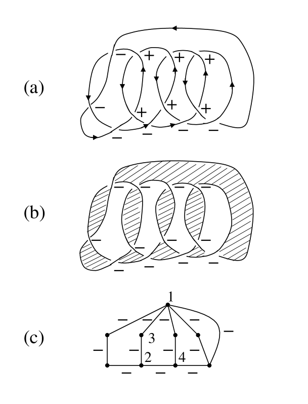
Figure 3: (a) A repeating chain knot with $3n$ crossings for $n=4$. Signs of crossings are those associated with oriented knots. (b) A shading of alternate faces. Signs of crossings are those determined by the topology of the shading relative to the crossings (see text). (c) The resulting Potts model lattice for the face shading in (b). Labellings 1, 2, 3, 4 are those given in (12).

To evaluate the partition function $Z_{n}(q;e^{K_{-}})$ for this Potts model, we define

$$F_{m}(\sigma_{1},\sigma_{2})=a_{m}+b_{m}\delta_{\rm Kr}(\sigma_{1},\sigma_{2}),\hskip 28.45274ptm=0,1,2,...$$ (11)

and the recursion relation

$$F_{m+1}(\sigma_{1},\sigma_{2}) = \Big{[}\sum_{\sigma_{3}=1}^{q}B(\sigma_{1},\sigma_{3})B(\sigma_{3},\sigma_{2})\Big{]}\cdot\Big{[}\sum_{\sigma_{4}=1}^{q}B(\sigma_{2},\sigma_{4})F_{m}(\sigma_{4},\sigma_{1})\Big{]}$$ (12)

$$\hskip 85.35826pt\hskip 28.45274ptm=0,1,2,...$$

obtained from a perusal of Fig. 3(c), with the initial condition $(a_{0},b_{0})=(0,1)$. The Potts partition function is then given by

$$Z(q;e^{K_{-}})=\sum_{\sigma_{1}=1}^{q}\sum_{\sigma_{2}=1}^{q}F_{n}(\sigma_{1},\sigma_{2})=q(qa_{n}+b_{n})$$ (13)

It therefore remains to compute $a_{n}$ and $b_{n}$.

To compute $a_{n}$ and $b_{n}$, we rewrite the recursion relation (12) as

$$\pmatrix{a_{m+1}\cr b_{m+1}}=\pmatrix{T_{11}&T_{12}\cr T_{21}&T_{22}\cr}\pmatrix{a_{m}\cr b_{m}},\hskip 28.45274ptm=0,1,2,...$$ (14)

where

$$T_{11} = (q-2+2e^{K_{-}})(q-1+e^{K_{-}})$$

$$T_{12} = q-2+2e^{K_{-}})$$

$$T_{21} = (e^{K_{-}}-1)^{2}(q-1+e^{K_{-}})$$

$$T_{12} = e^{K_{-}}(1-e^{K_{-}})^{2}-(1-e^{K_{-}})(q-2+2e^{K_{-}}).$$ (15)

Let $\lambda_{1}$ and $\lambda_{2}$ be the eigenvalues of the $2\times 2$ matrix in (14). After some straightforward manipulation, we arrive at the expression

$$\pmatrix{a_{n}\cr b_{n}\cr}={1\over{\lambda_{1}-\lambda_{2}}}\pmatrix{a_{0}(\lambda_{1}^{n+1}-\lambda_{2}^{n+1})+(b_{0}T_{12}-a_{0}T_{22})(\lambda_{1}^{n}-\lambda_{2}^{n})\cr b_{0}(\lambda_{1}^{n+1}-\lambda_{2}^{n+1})+(a_{0}T_{21}-b_{0}T_{11})(\lambda_{1}^{n}-\lambda_{2}^{n})}$$ (16)

Now we substitute with $(a_{0},b_{0})=(0,1),q=t+2+t^{-1}$ and $e^{K_{-}}=-t$, and obtain the eigenvalues

$$\lambda_{1} = -t^{-1}(1+t)^{2}$$

$$\lambda_{2} = t^{-2}(1+t)^{2}(1-t+t^{2}-t^{3}).$$ (17)

This leads to the partition function

$$Z(q;e^{K_{-}})={{(1+t^{-1})^{2n}}\over{1+t^{2}-t^{3}}}\Big{[}(-t)^{n+2}+(1-t^{3})(1-t+t^{2}-t^{3})^{n}\Big{]}$$ (18)

Substituting (18) into (3) with $M=2n+1,N=3n$ and making use of (10), we obtain the Jones polynomial

$$V_{K}(t)={{t^{-(n+3)}}\over{1+t^{2}-t^{3}}}\Big{[}t^{n+2}-(t^{3}-1)(t-1)^{n}(t^{2}+1)^{n}\Big{]},\hskip 14.22636ptn=1,2,...$$ (19)

The zeroes of $V_{K}(t)$ are now the roots of the equation

$$t^{n+2}-(t^{3}-1)(t-1)^{n}(t^{2}+1)^{n}=0$$ (20)

minus the three roots of $1+t^{2}-t^{3}=0$.

We have evaluated the roots of (20) in the complex $t$ plane numerically for $n\leq 23$, and present the results for typical values of $n$ in Fig. 4, and for all $n\leq 23$ in Fig. 5(a). It is seen that the zeroes generally fall on three closed curves centered about the points $1$, $i$ and $-i$. In addition, there are two isolated zeroes located near $t_{+}$ and $t_{-}$ and approaching $t_{\pm}$ as $n\to\infty$.

Figure 4: Distribution of zeroes for the repeating chain knot for fixed $n$.

To determine the loci of the closed curves, we solve $t^{n}$ from (20) and obtain, after taking the $n$-th root,

$${{(t-1)(t^{2}+1)}\over t}=\Bigg{|}{{t^{2}}\over{t^{3}-1}}\Bigg{|}^{1/n}\omega^{\alpha},\hskip 28.45274pt\alpha=1,2,...,n.$$ (21)

Thus, in the limit of $n\to\infty$ and $t^{3}\not=1$, the zeroes are distributed continuously on the three loci which are the roots of the cubic equation

$$(t-1)(t^{2}+1)=t\ e^{i\theta},\hskip 28.45274pt0\leq\theta<2\pi.$$ (22)

The loci (22) coincides with the crossover of the two eigenvalues, namely,

$$\big{|}\lambda_{1}\big{|}=\big{|}\lambda_{2}\big{|}$$ (23)

so that the Jones polynomial is nonanalytic at (22). The three loci are plotted in Fig. 5(b).

Figure 5: (a) Distribution of zeroes for the repeating chain knot for $n\leq 23$. (b) Distribution of zeroes for the repeating chain knot of in the limit of $n\to\infty$. The three loci are given by (22).

In the neighborhood of $t_{\pm}$, we have $t^{3}\sim 1$ and write $t=t_{\pm}+\Delta$ for some small $|\Delta|$. Then, to the leading order of $|\Delta|$ (21) reads

$$\pm\sqrt{3}i=|3\Delta|^{-1/n}\ t\ \omega_{n}^{\alpha}.$$ (24)

Taking the absolute value of both sides, (24) has a solution

$$|\Delta|\sim 3^{-(n+2)/2}$$ (25)

consistent with the assumption of $|\Delta|$ being small. This leads to an additional isolated root near $t_{+}$ (and $t_{-}$) at a distance of the order of $3^{-(n+2)/2}$, a fact borne out by our numerical results. The two isolated roots approach the points $t_{\pm}$ on the unit circle as $n$ increases, and merges onto the unit circle in the limit of $n\to\infty$. The average distance of the roots on the loci to the unit circle is $0.2651$.

6 Summary and discussions

We have investigated the distribution of zeroes of the Jones polynomial for all prime knots with $N\leq 10$ crossings, the torus knot, and a repeating chain knot of $n$ sections for general $n$. It is intriguing to note that the zero distribution for prime knots shown in Fig. 1 resembles that of a Julia set. It would be of interest to further clarify the possibility of this connection.

We have also given the explicit relation which connects the Jones polynomial to an associated Potts model, and used it to evaluate the Jones polynomial of the repeating chain knot. While the examples considered here are limited in scope, it is hoped that further studies along this line can lead to further revelation of the analytic properties of the Jones polynomial.

Note added: After the completion of this work we have learned that X.-S. Lin has studied zeroes of several Jones polynomials [23]. His findings on the torus knot are in agreement with ours. We have also been informed by R. Shrock that zeroes of the Jones polynomial for certain repeating chain of alternate knots have been studied via its connection with the Tutte polynomial [24].

References

- [1] C. N. Yang and T. D. Lee, Statistical theory of equations of states and phase transitions I. Theory of condensation, Phys. Rev. 87, 404-409 (1952).
- [2] T. D. Lee and C.N. Yang, Statistical theory of equations of state and phase transitions. II. Lattice gas and Ising model, Phys. Rev. 87, 410-419 (1952).
- [3] M. E. Fisher, The Nature of Critical Points, in Lecture Notes in Theoretical Physics, vol. 7c, edited by W. E. Brittin, (University of Colorado Press, Boulder, 1965), pp. 1-159.
- [4] G. E. Andrews, The theory of Partitions, in Encyclopedia of Mathematics and Its Applications, Ed. G.-C. Rota, Addison-Wesley (1976) Chaps. 3 and 11.
- [5] P. A. MacMahon, Combinatory Analysis, Vol 2, Cambridge University Press, London; Reprinted by Chelsea, New York (1960).
- [6] H. Y. Huang and F. Y. Wu, The infinite-state Potts model and solid partitions of an integer, Int. J. Mod. Phys. B 11, 121-126 (1997).
- [7] G. E. Andrews, Math. Rev. 98c, 11145 (1998).
- [8] V. F. R. Jones, A polynomial invariant for links via von Neumann algebras, Bull. Amer. Math. Soc. 129, 103-112 (1985).
- [9] V. F. R. Jones, On knot invariants related to some statistical mechanical models, Pacific J. Math. 137, 311-334 (1989).
- [10] F. Y. Wu, Knot theory and statistical mechanics, Rev. Mod. Phys. 64, 1099-1131 (1992).
- [11] J. M. Maillard and R. Rammal, Some analytical consequences of the inversion relation for the Potts model, J. Phys A 16, 353-367 (1983).
- [12] C. N. Chen, C. K. Hu, and F. Y. Wu, Partition function zeroes of the square lattice Potts model, Phys. Rev. Lett. 76, 169-172 (1996).
- [13] R. Shrock, Exact Potts model partition functions on ladder graphs, Physica A 283, 388-440 (2000), and references contained therein.
- [14] R. J. Baxter, Chromatic polynomials of large triangular lattices, J. Phys. A 20, 5241-5261 (1987).
- [15] R. Shrock and S. H. Tsai, Ground-state degeneracy of Potts antiferromagnets on two-dimensional lattices: Approach using infinite cyclic strip graphs, Phys. Rev. E 60, 3512-3515 (1999), and references contained there in.
- [16] R. B. Potts, Some generalized order-disorder transformations, Proc. Camb. Philos. Soc. 48, 106-109 (1952).
- [17] W. T. Tutte, A contribution to the theory of chromatic polynomials, Can. J. Math. 6, 80-91 (1954).
- [18] G. D. Birkhoff, A determinant formula for the number of ways of coloring of a map, Ann. Math. 14, 42-46 (1912).
- [19] H. N. V. Temperley and E. H. Leib, Relations between the percolation ad colouring problem and other graph-theoretical problems associated with regular planar lattices: some exact results for the percolation problem, Proc. Roy. Soc. London A 332, 251-280 (1071).
- [20] F. Y. Wu and Y. K. Wang, Duality transformation in a many-component spin model, J. Math. Phys. 17, 439-440 (1976).
- [21] V. F. R. Jones, Hecke algebra representation of braid groups and link polynomials, Ann. Math. 126 335-388 (1987).
- [22] L. H. Kauffman and F. Y. Wu, unpublished.
- [23] X. S. Lin and O. Dasbach, private communication.
- [24] S. C. Chang and R. Shrock, Zeroes of Jones polymials for families of knots and links, arXiv: math-ph/0103043.