Non-Gaussian equilibrium in a long-range Hamiltonian system
Abstract
We study the dynamics of a system of N classical
spins with infinite-range interaction.
We show that, if the thermodynamic limit is taken before the
infinite-time limit, the system does not relax to the
Boltzmann-Gibbs equilibrium,
but exhibits different equilibrium properties,
characterized by stable non-Gaussian velocity distributions,
Lévy walks and dynamical correlation in phase-space.
PACS numbers: 05.50.+q, 05.70.Fh, 64.60.Fr
Though not always clearly stated, standard equilibrium thermodynamics [1, 2, 3] is valid only for sufficiently short-range interactions. This is not the case, for example, for gravitational or unscreened Coulombian fields, or for systems with long-range microscopic memory and fractal structures in phase space. The increasing experimental evidence of dynamics and thermodynamics anomalies in turbulent plasmas [4] and fluids [5, 6, 7] , astrophysical systems [8, 9, 10, 11, 12], nuclei [13, 14] and atomic clusters[15], granular media[16], glasses[17, 18] and complex systems[19, 20] found in the last years, provide further motivation for a generalization of thermodynamics.
In this paper we consider a simple model of classical spins with infinite range interactions[21, 22, 23, 24], and we show that, if the thermodynamic limit is performed before the infinite time limit, the system does not relax to the Boltzmann-Gibbs (BG) equilibrium, but exhibits different equilibrium properties characterized by non-Gaussian velocity distributions, Lévy walks and dynamical correlation in phase-space, and the validity of the zeroth principle of thermodynamics. Our results show some consistency with the predictions of a generalized non-extensive thermodynamics recently proposed[25, 26]. The Hamiltonian Mean Field (HMF) model describes a system of N planar classical spins interacting through an infinite-range potential[21]. The Hamiltonian can be written as:
| (1) |
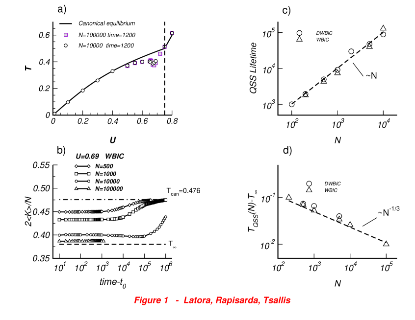
where is the angle and the conjugate variable representing the angular momentum (or the rotational velocity since unit mass is assumed). The interaction is the same as in the ferromagnetic X-Y model [2], though the summation is extended to all couples of spins and not restricted to first neighbors. Following tradition, the coupling constant in the potential is divided by N. This makes H only formally extensive ( when )[25, 26, 27, 28], since the energy remains non-additive, i.e. the system cannot be trivially divided in two independent sub-systems. The canonical analytical solution of the model predicts a second-order phase transition from a low-energy ferromagnetic phase with magnetization (M is the modulus of , where , to a high-energy one where the spins are homogeneously oriented on the unit circle and . The caloric curve, i.e. the dependence of the energy density on the temperature , is given by and shown in Fig.1(a). The critical point is at energy density corresponding to a critical temperature [21]. The dynamical behavior of HMF can be investigated in the microcanonical ensemble by starting the system with water bag initial conditions (WBIC), i.e. for all () and velocities uniformly distributed, and integrating numerically the equations of motion [22]. As shown in Fig.1(a), microcanonical simulations are in general in good agreement with the canonical ensemble, except for a region below , where it has also been found a dynamics characterized by Lévy walks, anomalous diffusion [23] and a negative specific heat[24]. Ensemble inequivalence and negative specific heat have also been found in self-gravitating systems [8], nuclei and atomic clusters [13, 14, 15], though in the present model such anomalies emerge as dynamical features [29, 30]. In order to understand better this disagreement we focus on a particular energy value, namely , and we follow the time evolution of temperature, magnetization, and velocity distributions.
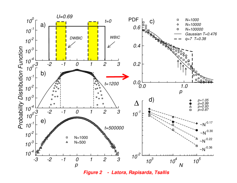
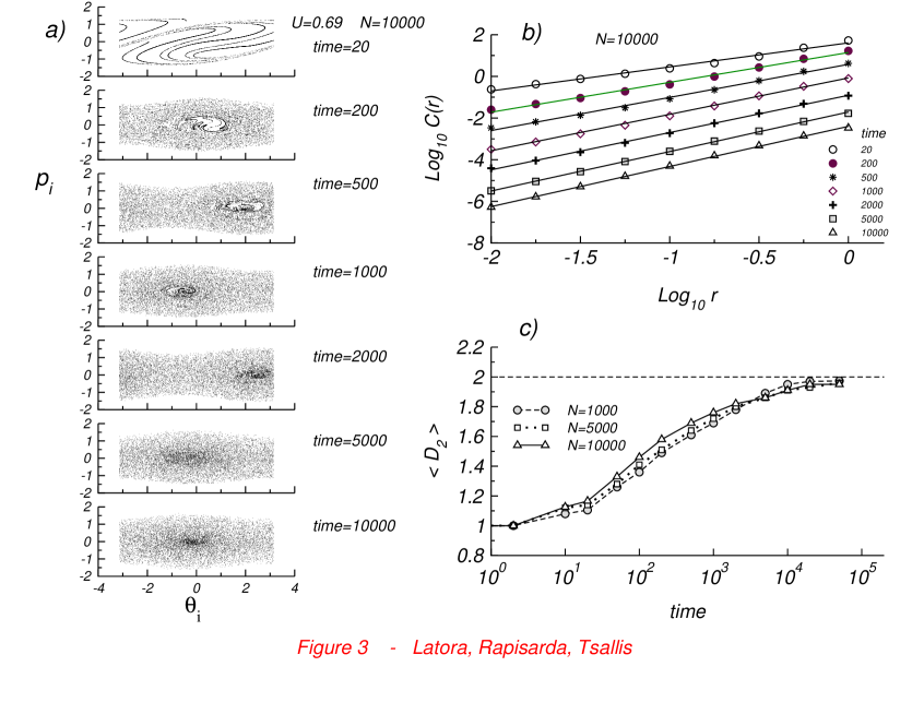
In Fig.1(b) we report the time evolution of , a quantity that, evaluated at equilibrium, is expected to coincide with the temperature ( denotes time averages). The system is started with WBIC and rapidly reaches a metastable or quasi-stationary state (QSS) which does not coincide with the canonical prediction. In fact, after a short transient time, shows a plateau corresponding to a N-dependent temperature (and ) lower than the canonical temperature. This metastable state needs a long time to relax to the canonical equilibrium state with temperature and magnetization . The duration of the plateau increases with the size of the system: in particular we have checked that the lifetime of QSS has a linear dependence on N, see Fig.1(c). Therefore the two limits and do not commute and if the thermodynamic limit is performed before the infinite time limit, the system does not relax to the BG equilibrium. This has been conjectured to be an ubiquitous feature in non-extensive systems[25], but it has also been found for spin glasses[17]. When N increases tends to , a value obtained analytically as the metastable prolongation (at energies below ) of the high-energy solution (). We have also found that and , see Fig. 1(d). At the same time we have checked that increasing the size, the largest Lyapunov exponent for the QSS tends to zero. In this sense mixing is negligible and one expects anomalies in the relaxation process [31]. The fact that converges to a nonzero value of temperature for means that, when N is macroscopically large, systems can share the same temperature, though this equilibrium is not the familiar one. All this amounts to say that the zeroth principle of thermodynamics is stronger than what one might think through BG statistical mechanics, since it is true even when the system is not at the usual BG equilibrium. We have checked the robustness of the above results by changing the level of accuracy of the numerical integration and by adding small perturbations. We also verified that the QSS has a finite basin of attraction, by adopting different initial conditions, as for example double water bag (DWBIC). In Fig.2 we focus on the velocity probability distribution functions (pdfs). The initial velocity pdfs (WBIC or DWBIC) , reported in Fig. 2(a) , quickly acquire and maintain during the entire duration of the metastable state a non-Gaussian shape , see Figs.2(b) and 2(c). The velocity pdf of the QSS is wider than a Gaussian for small velocities, but shows a faster decrease for . The enhancement for velocities around is consistent with the anomalous diffusion and the Lévy walks (with average velocity ) observed in the QSS regime [23]. The following rapid decrease for is due to conservation of total energy . The stability of the QSS velocity pdf can be explained by the fact that, for , and thus the force on the spins tends to zero with N, being . Of course, for finite N, we have always a small random force, which makes the system eventually evolve into the usual Maxwell-Boltzmann distribution after some time. We show this for small systems (N=500,1000) at time t=500000 in Fig.2(e). When this happens, Lévy walks disappear and anomalous diffusion leaves place to Brownian diffusion[23] . A possible frame to reproduce the non-Gaussian pdf in Fig.2 (b) could be the non-extensive statistical mechanics recently proposed[25, 26] with the entropic index . This formalism provides, for the canonical ensemble, a q-dependent power-law distribution in the variables , . This distribution has to be integrated over all and all but one in order to obtain the one-momentum pdf, , to be compared with the numerical one, , obtained by considering, within the present molecular dynamical frame, increasingly large N-sized subsystems of an increasingly large M-system. Within the numerical limit, we expect to go from the microcanonical ensemble to the canonical one (the cut-off is then expected to gradually disappear as indeed occurs in the usual short-range Hamiltonians), thus justifying the comparison between and . The enormous complexity of this procedure made us to turn instead onto a naive, but tractable, comparison, namely that of our present numerical results with the following one-free-particle pdf [25] , which recovers the Maxwell-Boltzmann distribution for . This formula has been recently used to describe successfully turbulent Couette-Taylor flow [5] and non-Gaussian pdfs related to anomalous diffusion of Hydra cells in cellular aggregates [19]. In our case, the best fit is obtained by a curve with , as shown in Figs. 2 (b) and 2 (c). The agreement between numerical results and theoretical curve improves with the size of the system. A finite-size scaling confirming the validity of the fit is reported in panel (d), where , the difference between the numerical results and the theoretical curve for , is shown to go to zero as a power of N (for four values of p). Since , the theoretical curve does not have a finite integral and therefore it needs to be truncated with a sharp cut-off to make the total probability equal to one. It is however clear that, the fitting value is only an effective non-extensive entropic index. Similar non-Gaussian pdfs have also been found in turbulence and granular matter experiments [5, 16], though this is the first evidence in a Hamiltonian system. In Fig.3 we verify, through the calculation of the fractal dimension [32], that a dynamical correlation emerges in the -space before the final arrival to a quasi-uniform distribution. During intermediate times some filamentary structures appear, a similar feature has recently been found also in self-gravitating systems[11], which might be closely related to the plateaux observed in Fig.1(b). We learn from the curves in Fig.3(c) that, since they do not sensibly depend on N, the possible connection does not concern the entire -space, but perhaps only the small sticky regions between the ”chaotic sea” and the quasi-orbits[33].
Metastable states are ubiquitous in nature. Their full understanding is, however, far from trivial. They basically correspond to local, instead of global, minima of the relevant thermodynamic energy. The two types of minima are separated by activation barriers which, at the thermodynamic limit, can be low, high or infinite, all of them presumably occurring in nature. The last case yields of course to quite drastic consequences. Moreover, the local minimum can either make the system to live in a smooth part of the a priori accessible phase space, or it can force it to live in a geometrically more complex (e.g., multifractal) part of the phase space. The richness of such situation is what makes interesting the study of glasses, nuclei, atomic clusters, self-gravitating and other complex systems. It is natural to expect for such systems that the infinite size and infinite time limits are not interchangeable. What has emerged quite clearly here is that thermodynamically large systems with long-range interactions belong to this very rich class. We have verified that the usual attributes of thermal equilibrium: zeroth principle at finite temperatures, robustness associated with a finite basin of attraction in the space of the initial conditions, stable distribution of velocities, are satisfied, but they systematically differ from what BG statistical mechanics has make familiar to us along the last 130 years. Our findings indicate some consistency with the predictions of non-extensive statistical mechanics [25], though a firm and unambiguous connection remains a challenge for future studies. In particular we believe all these features not to be exclusive of the present HMF model. Similar scenarios are expected for systems with say two-body interactions decaying like for , where is equal, for classical systems, to the space dimension [27, 28].
We thank M. Antoni, F. Baldovin, M. Baranger, E.P. Borges, E.G.D. Cohen, X. Campi, H. Krivine, M. Mézard, S. Ruffo and A. Torcini for stimulating discussions.
E-mail: vito.latora@ct.infn.it
E-mail: andrea.rapisarda@ct.infn.it
E-mail: tsallis@cbpf.br
REFERENCES
- [1] R.K. Pathria, Statistical Mechanics , Butterworth Heinemann (1996).
- [2] H.E. Stanley, Introduction to Phase Transitions and Critical Phenomena, Oxford University Press, New York (1971).
- [3] P.T. Landsberg, Thermodynamics and Statistical Mechanics , Dover (1991).
- [4] B.M. Boghosian, Phys. Rev. E 53 (1996) 4754.
- [5] C. Beck, G.S. Lewis and H.L. Swinney , Phys. Rev. E 63 (2001) 035303(R). See also C. Beck, Physica A 295 (2001) 195 and [cond-mat/0105374].
- [6] T.H.Solomon, E.R. Weeks and H.L. Swinney, Phys. Rev. Lett. 71 (1993) 3975.
- [7] M.F. Shlesinger, G.M. Zaslavsky and U. Frisch Eds., Lévy flights and related topics, Springer-Verlag Berlin (1995).
- [8] D. Lynden-Bell , Physica A 263 (1999) 293.
- [9] F. Sylos Labini, M. Montuori and L. Pietronero, Phys. Rep. 293 61 (1998) 61.
- [10] L. Milanovic, H.A.Posch and W. Thirring, Phys. Rev. E 57 (1998) 2763.
- [11] H. Koyama and T. Konishi, Phys. Lett. A 279 (2001) 226.
- [12] A. Torcini and M. Antoni, Phys. Rev. E 59 (1999) 2746.
- [13] D.H.E Gross, Microcanonical thermodynamics: Phase transitions in Small systems, 66 Lectures Notes in Physics, World scientific, Singapore (2001) and refs. therein.
- [14] M. D’Agostino et al., Phys. Lett. B 473 (2000) 219.
- [15] M. Schmidt, R. Kusche, T. Hippler, J. Donges and W. Kronmueller, Phys. Rev. Lett. 86 (2001) 1191.
- [16] A. Kudrolli and J. Henry, Phys. Rev. E 62 (2000) R1489; Y-H. Taguchi and H. Takayasu, Europhys. Lett. 30 (1995) 499.
- [17] G. Parisi, Physica A 280 (2000) 115.
- [18] P.G. Benedetti and F.H. Stillinger, Nature 410 (2001) 259.
- [19] A. Upaddhyaya, J.P. Rieu, J.A. Glazier and Y. Sawada, Physica A 293 (2001) 549.
- [20] G.M. Viswanathan , V. Afanasyev , S.V. Buldyrev, E.J. Murphy and H.E. Stanley, Nature 393 (1996) 413.
- [21] M. Antoni and S.Ruffo, Phys. Rev. E 52 (1995) 2361.
- [22] V. Latora , A. Rapisarda and S. Ruffo, Phys. Rev. Lett. 80 (1998) 692; Physica D 280 (1999) 81 and Progr. Theor. Phys. Suppl. 139 (2000) 204.
- [23] V. Latora, A. Rapisarda and S. Ruffo, Phys. Rev. Lett. 83 (1999) 2104 and Physica A 280 (2000) 81.
- [24] V. Latora and A. Rapisarda, Nucl. Phys. A 681 (2001) 331c.
- [25] C. Tsallis, J. Stat. Phys. 52, (1988) 479; for an updated review see: C. Tsallis, Nonextensive Statistical Mechanics and Thermodynamics , Lecture Notes in Physics, eds. S. Abe and Y. Okamoto, Springer, Berlin, (2001).
- [26] J.A.S. Lima, R. Silva and A.R. Plastino, Phys. Rev. Lett. 86 (2001) 2938.
- [27] C. Anteneodo and C. Tsallis , Phys. Rev. Lett. 80 (1998) 5313; F. Tamarit and C. Anteneodo, Phys. Rev. Lett. 84 (2000) 208.
- [28] A. Campa, A. Giansanti and D. Moroni, Phys. Rev. E 62 (2000) 303 and Chaos Solitons and Fractals (2001) in press [cond-mat/0007422].
- [29] M. Antoni, H. Hinrichsen and S. Ruffo, Chaos Solitons and Fractals (2001) in press [cond-mat/9810048].
- [30] V. Latora and A. Rapisarda, Chaos Solitons and Fractals (2001) in press [cond-mat/0006112].
- [31] N.S. Krylov, Nature 153 (1944) 709.
- [32] P. Grassberger and I. Procaccia, Phys. Rev. Lett. 50 (1983) 346.
- [33] M.F. Shlesinger, G.M. Zaslavsky and J. Klafter, Nature 363 (1993) 31.