Reorientation phase transitions in thin magnetic films: a review of the classical vector spin model within the mean field approach

Abstract

The ground state and the finite temperature phase diagrams with respect to magnetic configurations are studied systematically for thin magnetic films in terms of a classical Heisenberg model including magnetic dipole-dipole interaction and uniaxial anisotropy. Simple relations are derived for the occurrence of the various phase boundaries between the different regions of the magnetic orientations. In particular, the range of the first and second order reorientation phase transitions are determined for bi- and trilayers.

1 Introduction

Recent developments of thin film technologies enable the control of the growth of ultrathin magnetic films deposited on nonmagnetic substrates. Due to their challenging application as high-storage magnetic recording media, much attention Gradmann (1986), Allenspach et al. (1990), Pappas et al. (1990, 1992), Allenspach (1994), Li et al. (1994), Berger and Hopster (1996), Garreau et al. (1996), Farle et al. (1997), Gubiotti et al. (1997) has been devoted to the novel properties of these new structures. From a technological point of view, the study of the magnetic phase transitions, in particular, of reorientations of the magnetisation is playing a major role. As compared to bulk systems, the presence of surfaces and interfaces leads to an enhancement of the magneto-crystalline anisotropy due to spin–orbit coupling. The magneto-crystalline anisotropy often prefers a magnetisation perpendicular to the surface, while the magnetic dipole–dipole interaction and the entropy at finite temperatures favor an in–plane magnetisation. Consequently, as observed in many Fe or Co based ultrathin films Gradmann (1986), Allenspach et al. (1990), Pappas et al. (1990, 1992), Allenspach (1994), Li et al. (1994), Berger and Hopster (1996), Garreau et al. (1996), a reorientation from out–of–plane to an in–plane direction of the magnetisation occurs by increasing both the thickness of the film or the temperature. Relativistic first principles calculations using the local spin density approximation (LSDA) turned out to be sufficiently accurate to reproduce the critical thickness of the reorientation Szunyogh et al. (1995, 1997b), Zabloudil et al. (1998).

In the case of thin Ni films deposited on a Cu(001) surface, an opposite behavior was revealed: the magnetisation was found to be in-plane for less than 7 Ni monolayers, however, it became perpendicular to the surface beyond this thickness. Below the switching thickness near 0 K, even an increase of the temperature induces a similar reversed reorientation Farle et al. (1997), Gubiotti et al. (1997). The main origin of the above reorientation was attributed to a strain induced anisotropy of the inner layers preferring a perpendicular magnetisation Hjortstam et al. (1997), Uiberacker et al. (1999).

Subsequent to the pioneering works of Mills (1989), who predicted the existence of a canted non-collinear ground state for a semi–infinite ferromagnetic system, and that of Pescia and Pokrovsky (1990) who, by using a renormalization group treatment of a continuum vector field model, for the first time described the temperature induced (normal) reorientation phase transition, a considerable amount of theoretical attempts, mostly by means of different statistical spin models, was suggested in order to explain the above findings for the thickness and temperature driven reorientation transitions. In some attempts, classical vector spin models were used within the mean field approximation Taylor and Györffy (1993), Hucht and Usadel (1996, 1997, 1999a, 1999b, 2000), Jensen and Bennemann (1998), Hu et al. (1999) or in terms of Monte Carlo simulations Taylor and Györffy (1993), Serena et al. (1993), Chui (1995), Hucht et al. (1995), Hucht and Usadel (1996), MacIsaac et al. (1996). A quantum–spin description of reorientation transitions has also been provided in terms of spin–wave theory Bruno (1991), mean field theory Moschel and Usadel (1994, 1995), many–body Green function techniques Fröbrich et al. (2000a, b), Jensen et al. (2000), and by using Schwinger bosonization Timm and Jensen (2000). Although, the mean field theory is not expected to give a sufficiently accurate description of low–dimensional systems, it turned out, that it is a successful tool to study spin reorientation transitions and yields qualitatively correct predictions Moschel and Usadel (1994, 1995), Hucht and Usadel (1997, 1999a, 1999b, 2000), Jensen and Bennemann (1998), Hu et al. (1999). It also should be noted that an itinerant electron Hubbard model revealed the sensitivity of reorientation transitions with respect to electron correlation effects Herrmann et al. (1998).

For layered systems, the following simple model Hamiltonian can be used to study reorientation transitions, see e.g. Taylor and Györffy (1993),

$$H= -{1\over 2}\sum_{(p,i),(q,j)}^{NN}\!\!J\>\mathbf{s}_{pi}\cdot\mathbf{s}_{qj}-\sum_{p,i}\lambda_{p}(s_{pi}^{z})^{2}$$ (1)

$$+{1\over 2}\sum_{(p,i)\neq(q,j)}\!\!\omega\left[{\mathbf{s}_{pi}\cdot\mathbf{s}_{qj}\over r_{pi,qj}^{3}}-3{(\mathbf{s}_{pi}\cdot\mathbf{r}_{pi,qj})(\mathbf{s}_{qj}\cdot\mathbf{r}_{pi,qj})\over r_{pi,qj}^{5}}\right]\;,$$

where $\mathbf{s}_{pi}$ ($\mid\!\mathbf{s}_{pi}\!\mid=1)$ is a classical vector spin at lattice position $i$ in layer $p$ and $\mathbf{r}_{pi,qj}$ is a vector pointing from site $(p,i)$ to site $(q,j)$ measured in units of the two–dimensional (2D) lattice constant of the system, $a$. Although our previous calculations of the Heisenberg exchange parameters in thin Fe, Co and Ni films on Cu(001) showed some layer–dependence Szunyogh and Udvardi (1998, 1999), in the first term of Eq. (1) we only consider a uniform nearest neighbor (NN) coupling parameter $J$ throughout the film. Similarly, as we neglect the well–known surface/interface induced enhancement of the spin–moments, we use a single parameter $\omega=\mu_{0}\mu^{2}/4\pi a^{3}$ (with $\mu_{0}$ the magnetic permeability and $\mu$ an average magnitude of the spin–moments), characterizing the magnetic dipole-dipole interaction strength in the third term of Eq. (1). As revealed also by first principles calculations – see Weinberger and Szunyogh (2000) and references therein – , the uniaxial magneto–crystalline anisotropy depends very sensitively on the type of the surface/interface, the layer–wise resolution of which can vary from system to system. Therefore, the corresponding parameters, $\lambda_{p}$, in the second term of Eq. (1) remain layer dependent: the variety of these anisotropy parameters leads to rich magnetic phase diagrams covering the experimentally detected features mentioned above. For example, in a previous study Udvardi et al. (1998) we pointed out that, even in the absence of a fourth order anisotropy term, for a very asymmetric distribution of $\lambda_{p}$ with respect to the layers, the Heisenberg model in Eq. (1) can yield a canted (non-collinear) ground state. This feature cannot be obtained within a phenomenological single domain picture.

As what follows, we first investigate the possible ground states of the Hamiltonian, E q. (1). Then we perform a systematic mean field study of the different kind of temperature induced reorientation transitions, devoting special attention to the case of bi– and trilayers. Specifically, we define general conditions for the reversed reorientation. Most authors in the past focused on proving the existence of different reorientations and detected only some parts of the phase diagram, where first and second order phase transitions occurred. In here, we describe the full range of uniaxial anisotropies ($\lambda_{p}$), for which first or second order reorientation phase transitions can exist. Finally, we attempt to summarize the results and impacts of a mean field approach.

2 Ground state

Confining ourselves to spin–states in which the spins are parallel in a given layer, but their orientations may differ from layer to layer, i.e.

$$\mathbf{s}_{pi}=\mathbf{s}_{p}=\left(\sin(\theta_{p})\cos(\phi_{p}),\sin(\theta_{p})\sin(\phi_{p}),\cos(\theta_{p})\right)\quad,$$ (2)

where $\theta_{p}$ and $\phi_{p}$ are the usual azimuthal and polar angles with the $z$ axis normal to the planes, the energy of $N$ layers per 2D unit cell can be written as

$$E_{N}(\theta_{1},\theta_{2},\dots,\theta_{N};\phi_{1},\phi_{2},\dots,\phi_{N})=-{1\over 2}\sum_{p,q=1}^{N}(Jn_{pq}-A_{pq}\omega)\cos{(\theta_{p})}\cos{(\theta_{q})}$$ (3)

$$-{1\over 2}\sum_{p,q=1}^{N}(Jn_{pq}+{1\over 2}A_{pq}\omega)\sin{(\theta_{p})}\sin{(\theta_{q})}\cos(\phi_{p}-\phi_{q})-\sum_{p=1}^{N}\lambda_{p}\cos^{2}{(\theta_{p})}\quad,$$

with $n_{pq}$ being the number of nearest neighbors in layer $q$ of a site in layer $p$, and $A_{pq}$ the magnetic dipole–dipole coupling constants, see Appendix in Szunyogh et al. (1995),

$${\sum_{j}}^{\prime}\frac{1}{r_{p0,qj}^{3}}\left(I-3{\mathbf{r}_{p0,qj}\otimes\mathbf{r}_{p0,qj}\over r_{p0,qj}^{2}}\right)=A_{pq}\times\left(\begin{array}[]{ccc}-{1\over 2}&0&\;0\\ 0&-{1\over 2}&\;0\\ 0&0&\;1\\ \end{array}\right)\quad,$$ (4)

which is valid for square and hexagonal 2D lattices, such as the (100) and (111) surfaces of cubic systems. ($I$ the three dimensional unit matrix, while $\otimes$ stands for the tensorial product of two vectors.) For three–dimensional (3D) translational invariant underlying parent lattices Weinberger (1997), $A_{pq}$ depends only on $|p-q|$, i.e. the distance between layers $p$ and $q$. In table 1 we summarize these constants for the first few layers of the most common cubic structures. As the magnetic dipole–dipole interaction is clearly dominated by the positive first (and second) layer couplings, for ferromagnetic systems ($J>0$), a minimum of the energy in Eq. (3) corresponds to the case when all polar angles, $\phi_{p}$, are identical. Therefore, the $\phi$–dependence in Eq. (3) disappears and the expression,

$$E_{N}(\theta_{1},\theta_{2},\dots,\theta_{N})= -{1\over 2}\sum_{p,q=1}^{N}(Jn_{pq}-A_{pq}\omega)\cos{(\theta_{p})}\cos{(\theta_{q})}$$ (5)

$$-{1\over 2}\sum_{p,q=1}^{N}(Jn_{pq}+{1\over 2}A_{pq}\omega)\sin{(\theta_{p})}\sin{(\theta_{q})}-\sum_{p=1}^{N}\lambda_{p}\cos^{2}{(\theta_{p})}\quad,$$

has to be minimized with respect to the $\theta_{p}$. The corresponding Euler–Lagrange equations are then

$${\partial E_{N}(\theta_{1},\theta_{2},\dots,\theta_{N})\over\partial\theta_{p}}= \ \ \,\sum_{q=1}^{N}(Jn_{pq}-A_{pq}\omega)\sin{(\theta_{p})}\cos{(\theta_{q})}$$ (6)

$$-\sum_{q=1}^{N}(Jn_{pq}+{1\over 2}A_{pq}\omega)\cos{(\theta_{p})}\sin{(\theta_{q})}$$

$$+2\lambda_{p}\sin{(\theta_{p})}\cos{(\theta_{p})}=0\;.$$

Obviously, a uniform in–plane ($\{\theta_{p}=\pi/2\}$) and a normal–to–plane ($\{\theta_{p}=0\}$) orientation satisfy Eq. (6). The energies of these two particular spin–states coincide, if

$$\sum_{p=1}^{N}{\lambda_{p}\over\omega}={3\over 4}\sum_{p,q=1}^{N}A_{pq}\;,$$ (7)

which defines an $(N\!-\!1)$–dimensional hyper–plane in the $N$–dimensional space of parameters $\{{\lambda_{p}/\omega}\}$. If the magnetisation changes continuously across this plane, in its vicinity there should exist solutions with canted magnetisation. Moreover, the saddle points of the energy functional in Eq. (5),

$$det\left|{\partial E_{N}\over\partial\theta_{p}\partial\theta_{q}}\right|_{\{\theta_{p}=0,{\pi\over 2}\}}=0\;,$$ (8)

define the boundaries of the canted zone,

$$det\left|\left[\sum_{r=1}^{N}\left({J\over\omega}n_{pr}+{1\over 2}A_{pr}\right)-2{{\lambda_{p}}\over{\omega}}\right]\delta_{pq}-\left({J\over\omega}n_{pq}-A_{pq}\right)\right|=0\;,$$ (9)

and

$$det\left|\left[\sum_{r=1}^{N}\left({J\over\omega}n_{pr}-A_{pr}\right)+2{{\lambda_{p}}\over{\omega}}\right]\delta_{pq}-\left({J\over\omega}n_{pq}+{1\over 2}A_{pq}\right)\right|=0\;,$$ (10)

for the uniform in–plane and normal–to–plane magnetisations, respectively. For a bilayer we derived explicit expressions of Eqs. (9) and (10), see Udvardi et al. (1998).

In order to study the canted region, instead of solving the Euler–Lagrange equations, Eq. (6), directly, we fixed a configuration $\theta_{1}^{\star},\theta_{2}^{\star}\dots\theta_{N}^{\star}$ and determined $\lambda_{1},\lambda_{2}\dots\lambda_{N}$ by demanding that Eq. (6) must be satisfied, i.e.

$$\lambda_{p}={1\over 2}\sum_{q=1}^{N}(Jn_{pq}+{1\over 2}A_{pq}\omega){\sin(\theta_{q}^{\star})\over\sin(\theta_{p}^{\star})}-{1\over 2}\sum_{q=1}^{N}(Jn_{pq}-A_{pq}\omega){\cos(\theta_{q}^{\star})\over\cos(\theta_{p}^{\star})}\;.$$ (11)

Substituting these parameters into Eq. (5), one easily can express the difference of the energies between the corresponding configurations as,

$$E_{N}(\theta_{1}=\theta_{2}=\dots=\theta_{N}=0)-E_{N}(\theta_{1}^{\star},\theta_{2}^{\star},\dots\theta_{N}^{\star})=$$ (12)

$${1\over 2}\sum_{pq}^{N}\left(n_{pq}J-A_{pq}\omega\right)\left[{\cos{(\theta_{p}^{\star})}\over\cos{(\theta_{q}^{\star})}}+{\cos{(\theta_{q}^{\star})}\over\cos{(\theta_{p}^{\star})}}-2\right],$$

and

$$E_{N}(\theta_{1}=\theta_{2}=\dots=\theta_{N}={\pi\over 2})-E_{N}(\theta_{1}^{\star},\theta_{2}^{\star},\dots\theta_{N}^{\star})=$$ (13)

$${1\over 2}\sum_{p,q}^{N}\left(n_{pq}J+{1\over 2}A_{pq}\omega\right)\left[{\sin{(\theta_{p}^{*})}\over\sin{(\theta_{q}^{*})}}+{\sin{(\theta_{q}^{*})}\over\sin{(\theta_{p}^{*})}}-2\right]\;.$$

Note that the position of the minimum $\{\theta_{p}^{\star}\}$ as well as the minimum energy $E_{N}(\{\theta_{p}^{\star}\})$ are functions of the parameters $J$, $\omega$, and $\{\lambda_{p}\}$. Obviously, whenever the parameters fall into the region between the two hyper–planes defined by Eqs. (9) and (10), the energy of non–collinear states is always below or equal to the energy of the collinear in-plane or normal–to–plane solutions.

We showed that for a bilayer, $\lambda_{1}=\lambda_{2}=3(A_{11}+A_{12})\omega/4$ implies a collinear ground state spin configuration Udvardi et al. (1998). This state is, however, continuously degenerate, i.e. the energy is independent of the orientation of the magnetisation. Such a critical point in the phase diagram also exists for multilayers ($N\geq 3$). Namely, from Eqs. (12) and (13) it follows that for $\theta_{1}^{\star}=\theta_{2}^{\star}\dots=\theta_{N}^{\star}=\theta^{\star}$, $E_{N}(\{\theta_{p}^{\star}\})$ is independent of $\theta^{\star}$. In terms of Eq. (11), the corresponding point in the parameter space $\{\lambda_{p}/\omega\}$ is given by

$${\lambda_{p}\over\omega}={3\over 4}\sum_{q=1}^{N}A_{pq}\;.$$ (14)

Evidently, the hyper–planes given by Eq. (9) and Eq. (10) touch the hyper–plane, separating the in–plane and normal–to–plane regions, Eq. (7), at the point defined by Eq. (14). It is worthwhile to mention that this is the only point where canted collinear solutions can exist. This critical point was also found by Hucht and Usadel (1996) for a monolayer, but they did not prove its existence for multilayers.

3 Finite temperature

Introducing the following coupling constants

$$c^{x}_{pq}=n_{pq}J+{1\over 2}\omega A_{pq}\quad{\rm and}\quad c^{z}_{pq}=n_{pq}J-\omega A_{pq}\;,$$ (15)

the molecular field corresponding to the Hamiltonian Eq. (1) at layer $p$ can be written as

$$H^{p}(\theta,\phi)= -\sum_{q=1}^{N}c^{x}_{pq}\left[m^{x}_{p}\sin{(\theta)}\cos{(\phi)}+m^{y}_{p}\sin{(\theta)}\sin{(\phi)}\right]$$ (16)

$$-\sum_{q=1}^{N}c^{z}_{pq}m^{z}_{q}\cos{(\theta)}-\lambda_{p}\cos^{2}{(\theta)}\;,$$

where $m^{\alpha}_{p}=\langle s^{\alpha}_{p}\rangle$ ($\alpha=x,y,z$). Similar to the ground state (see Section II.), due to the in–plane rotational symmetry of the above effective Hamiltonian, the in–plane projections of all the average magnetic moments $\mathbf{m}_{p}$ are aligned. Therefore, by choosing an appropriate coordinate system, $m^{y}_{p}$ can be taken to be zero in Eq. (16). The partition function is then defined by

$$Z=\prod_{p=1}^{N}Z_{p}\;,$$ (17)

$$Z_{p}=2\pi\int\limits_{-{\pi\over 2}}^{\pi\over 2}\exp\left\{\beta\left[b_{p}^{z}\cos(\theta)+\lambda_{p}\cos^{2}(\theta)\right]\right\}J_{0}(-i\beta b_{p}^{x}\sin(\theta))\sin(\theta)d\theta\;,$$ (18)

where

$$b^{x(z)}_{p}=\sum_{q=1}^{N}c^{x(z)}_{pq}m^{x(z)}_{q}\;,$$ (19)

$\beta=1/(k_{B}T)$, $k_{B}$ the Boltzmann–constant and $T$ the temperature. The minimization of the free–energy with respect to the average magnetisations leads to the following set of nonlinear equations

$$m_{p}^{x}={2i\pi\over Z_{p}}\int\limits_{-{\pi\over 2}}^{\pi\over 2}\sin(\theta)\exp\left\{\beta\left[b_{p}^{z}\cos(\theta)+\lambda_{p}\cos^{2}(\theta)\right]\right\}J_{1}(-i\beta b_{p}^{x}\sin(\theta))\sin(\theta)d\theta$$ (20)

and

$$m_{p}^{z}={2\pi\over Z_{p}}\int\limits_{-{\pi\over 2}}^{\pi\over 2}\cos(\theta)\exp\left\{\beta\left[b_{p}^{z}\cos(\theta)+\lambda_{p}\cos^{2}(\theta)\right]\right\}J_{0}(-i\beta b_{p}^{x}\sin(\theta))\sin(\theta)d\theta\;.$$ (21)

In Eqs. (17), (20) and (21), $J_{0}$ and $J_{1}$ denote Bessel functions of zero and first order, respectively Abramowitz and Stegun (1972).

By using a high temperatures expansion, Eqs. (20) and (21) become decoupled (see Appendix). Consequently, the magnetisation can go to zero either via an in–plane or via a normal–to–plane direction at temperatures $T_{x}$ and $T_{z}$, respectively, and the higher one of them can be associated with the Curie temperature $T_{C}$. Clearly, an out–of–plane to in–plane reorientation phase transition can occur only when the ground state magnetisation is out–of–plane and $T_{z}<T_{x}=T_{C}$. In the case of a reversed reorientation transition, the ground state magnetisation has to be in–plane (or canted) and $T_{x}<T_{z}=T_{C}$.

Expanding $T_{x}$ and $T_{z}$ up to first order of the anisotropy parameters $\lambda_{p}$, leads to the following expressions (see Appendix)

$$T_{x} ={1\over{3k_{B}}}\left[n_{11}J+{1\over 2}A_{11}\omega+2\left(n_{12}J+{1\over 2}A_{12}\omega\right)\cos\left({\pi\over N+1}\right)\right]$$ (22)

$$-{4\over{15(N+1)}}\sum_{p=1}^{N}\lambda_{p}\sin^{2}\left({p\pi\over N+1}\right)\;,$$

and

$$T_{z} ={1\over{3k_{B}}}\left[n_{11}J-A_{11}\omega+2\left(n_{12}J-A_{12}\omega\right)\cos\left({\pi\over N+1}\right)\right]$$ (23)

$$+{8\over{15(N+1)}}\sum_{p=1}^{N}\lambda_{p}\sin^{2}\left({p\pi\over N+1}\right)\;.$$

The above expressions imply that, if the anisotropy parameters $\lambda_{p}$ are small, $T_{x}$ is larger than $T_{z}$. As the anisotropy parameters are increasing, the difference between $T_{z}$ and $T_{x}$ decreases. The two temperatures coincide, if the following condition is fulfilled,

$$\sum_{p=1}^{N}\left({\lambda_{p}\over\omega}\right)\sin^{2}\left({p\pi\over N+1}\right)={{5(N+1)}\over 8}\left[A_{11}+2A_{12}\cos\left({\pi\over N+1}\right)\right]\;.$$ (24)

Above the hyper–plane determined by Eq. (24), i.e. for $T_{x}<T_{z}$, the uniaxial anisotropy is large enough to keep the magnetisation normal to the surface as long as the temperature reaches $T_{C}$.

First principles calculations on (Fe,Co,Ni)/Cu(001) overlayers revealed Újfalussy et al. (1996), Szunyogh et al. (1997a), Szunyogh and Udvardi (1998, 1999), Uiberacker et al. (1999), that the uniaxial magnetic anisotropy energy and the magnetic dipole–dipole interaction are two to three orders of magnitude smaller than the exchange coupling. Thus, for physically relevant parameters, the boundaries of the canted ground state fixed by Eqs. (9) and (10) are close to the hyper–plane defined by Eq. (7). Apart form this tiny range of canted ground states, temperature induced out–of–plane to in–plane reorientation can occur in the parameter space $\{\lambda_{p}/\omega\}$ between the two hyper–planes given by Eqs. (7) and (24). It is worthwhile to mention that the positions of these hyper–planes are determined only by the magnetic dipole–dipole constants $A_{pq}$.

An example for an out–of–plane to in–plane reorientation transition in a 5–layer thick film is shown in figure 1. Neglecting the fourth order anisotropy terms, the parameters of the system have been chosen identical to those characteristic to a Co₅/Au(111) overlayer Udvardi et al. (1998). Due to the highly asymmetric distribution of the $\lambda_{p}$ with respect to the layers, the system has a non–collinear canted ground state. As the temperature increases, the magnetisation in each layer turns into the plane of the film. The system keeps its non–collinear configuration up to the reorientation transition temperature ($\sim 0.9J/k_{B}$), above which it is uniformly magnetized in–plane up to the Curie temperature ($\sim 3.8J/k_{B}$).

The temperature induced reversed reorientation transition, found experimentally in Ni_n / Cu(001) films for $n<7$, has successfully been described by Hucht and Usadel (1997), who used a perturbative mean field approach to the model given in Eq. (1). Using the same parameters, we solved the mean field equations (20) and (21) and reproduced the reversed reorientation transition without any perturbative treatment. The results for a 4–layer film are shown in figures 2 and 3. Although the distribution of the anisotropy parameters is asymmetric, the calculation resulted in identical magnetisations in the first and fourth layer as well as in the second and third layer. Moreover, the angles of the magnetisations in the different layers are almost identical: in the whole temperature range the largest deviation is smaller than $6\times 10^{-4}$ rad.

For a bilayer ($N=2$) the hyper-planes (7) and (24) reduce to the lines

$${\lambda_{1}\over\omega}+{\lambda_{2}\over\omega}={3\over 2}\left(A_{11}+A_{12}\right)\quad{\rm and}\quad{\lambda_{1}\over\omega}+{\lambda_{2}\over\omega}={5\over 2}\left(A_{11}+A_{12}\right)\;,$$ (25)

respectively. Apparently, the two lines do not intersect. As a consequence, a reversed reorientation can occur only if the number of layers in the film exceeds two. The same conclusion has been drawn by Hucht and Usadel (1997) using a perturbative treatment of the anisotropy parameters. Nevertheless, it is interesting to note, that the region in the parameter space $\{\lambda_{p}/\omega\}$ of canted ground states, bounded by the lines defined by Eqs. (9) and (10), always overlaps the region, where the magnetisation goes to zero via in–plane orientation. Thus, in this overlapping region an out–of–plane (canted) to in–plane, i.e. reversed reorientation transition can indeed occur. The corresponding parameters, $\omega$ and $\{\lambda_{p}\}$, are, however, most likely beyond the physically relevant regime.

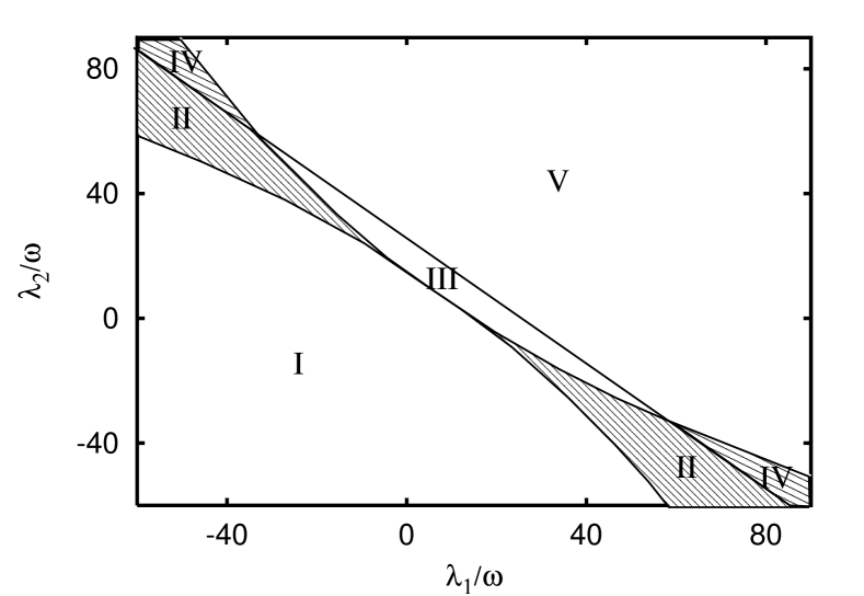
Figure 4: Phase diagram of the magnetic ground states and the reorientation phase transitions for a bilayer. The magnetic dipole–dipole coupling strength $\omega=0.01J$. I: in–plane magnetisation up to $T_{C}$; II: canted ground state with reorientation transition to in–plane orientation; III: normal–to–plane ground state with reorientation transition to in–plane orientation; IV: canted ground state with reversed reorientation transition; V: normal–to–plane magnetisation up to $T_{C}$.

For a bilayer, in figure 4 the different regions of phase transitions in the respective parameter space are shown. In regions I and V there is no temperature driven reorientation transition and the magnetisation remains in–plane and normal–to–plane, respectively, until $T_{C}$ is reached. In the regions II and III, the magnetisation turns into the plane from a canted or a normal–to–plane ground state, respectively. As discussed above, in region IV, a reversed reorientation can occur from a canted ground state to a normal–to–plane direction.

The order of the reorientation transition at finite temperatures has been studied in the literature by mean field and Monte Carlo methods. Most authors concluded Hucht et al. (1995), Hucht and Usadel (1996), MacIsaac et al. (1996) that the reorientation transition in a monolayer is of first order. For a bilayer, within the mean field approach, a relatively small range in the vicinity of $\lambda_{1}=\lambda_{2}$ was found, where the system underwent a first order reorientation transition Hucht and Usadel (1996). In what follows, we establish a simple, general criterion for the order of the reorientation transition. Suppose that the ground state magnetisation is in–plane and its normal–to–plane component appears at the temperature $T_{rz}$. Since near $T_{rz}$ the $z$–component of the magnetisation is small, the exponential function in Eq. (21) can be expanded up to first order in $m^{z}_{p}$, leading to the homogeneous linear equations

$$\sum_{q=1}^{N}C^{z}_{pq}m^{z}_{q}=0\quad,$$ (26)

where

$$C^{z}_{pq}\equiv\delta_{pq}-\beta_{rz}c^{z}_{pq}{\mathcal{Z}}_{p}\quad,$$ (27)

$${\mathcal{Z}}_{p}={2\pi\over Z_{p}}\int\cos^{2}(\theta)\exp\left[\beta_{rz}\lambda_{p}\cos(\theta)^{2}\right]J_{0}(-i\beta_{rz}b_{p}^{x}\sin(\theta))\sin(\theta)d\theta\quad,$$ (28)

and $\beta_{rz}\equiv 1/(k_{B}T_{rz})$. Note, that the $C^{z}_{pq}$ depend only on the in-plane component of the magnetisations $m^{x}_{q}$, which has to satisfy Eq. (20) for the case of $m^{z}_{q}=0$. Eq. (26) has a non-trivial solution only, if the determinant of the matrix $C^{z}=\left\{C^{z}_{pq}\right\}$ is zero. Evidently, this is the condition which determines $T_{rz}$. Similarly, one can easily find the corresponding equation for $T_{rx}$, where the in–plane component of the magnetisation appears in a normal–to–plane spin configuration,

$$\sum_{q=1}^{N}C^{x}_{pq}m^{x}_{q}=0\quad,$$ (29)

with

$$C^{x}_{pq}=\delta_{pq}-\beta_{rx}c^{x}_{pq}{\mathcal{X}}_{p}\quad,$$ (30)

$${\mathcal{X}}_{p}={\pi\over Z_{p}}\int\sin^{3}(\theta)\exp\left[\beta_{rx}\lambda_{p}\cos^{2}(\theta)\right]\left[J_{0}(-i\beta_{rx}b_{p}^{x}\sin(\theta))-J_{2}(-i\beta_{rx}b_{p}^{x}\sin(\theta))\right]d\theta\;,$$ (31)

and $\beta_{rx}\equiv 1/(k_{B}T_{rx})$. It is easy to show, that Eqs. (26) and (29) directly follow from a stability analysis of the mean field free energy in the vicinity, where the corresponding components of the magnetisations vanish.

The mean field equations, Eqs. (20) and (21), always have an in–plane and a normal–to–plane solution with magnetisations $m^{q}_{x}\neq 0$, $m^{q}_{z}=0$ and $m^{q}_{z}\neq 0$, $m^{q}_{x}=0$, respectively. Between $T_{rx}$ and $T_{rz}$, a canted solution can exist with $m^{q}_{x}\neq 0$ and $m^{q}_{z}\neq 0$. Among the above three phases, the physical one belongs to that, which has the lowest free–energy. In figure 5$a$, the free–energy of a system possessing a second order normal–to–plane to in–plane reorientation transition is schematically shown. The ground state magnetisation is perpendicular to the surface of the substrate. At $T_{rx}$ an in–plane component appears in the magnetisation. The normal–to–plane component of the magnetisation vanishes at the temperature $T_{rz}(>T_{rx})$. A similar picture for a first order transition is shown in figure 5b. Obviously, one can conclude that, if $T_{rx}<T_{rz}$, a second order normal–to–plane to in–plane reorientation phase transition occurs, whereas, if $T_{rz}<T_{rx}$, the reorientation transition is of first order. In the case of a reversed reorientation, the relation between $T_{rx}$ and $T_{rz}$ is just the opposite as before: a second order transition occurs, if $T_{rz}<T_{rx}$, while for $T_{rx}<T_{rz}$ the transition is of first order. At the boundary of the regions, where second order and first order phase transitions occur, the two temperatures, $T_{rx}$ and $T_{rz}$, must evidently coincide.

In figure 6, the region of first order reorientations (III F) and that of second order reorientations (III S) are shown in the phase diagram for a bilayer. Note, that figure 6 in fact represents figure 4 on an enlarged scale for the parameters $0<\lambda_{1,2}/\omega<18$. This picture is consistent with the observation of Hucht and Usadel (1996) for the range of the first order reorientation phase transitions, as they performed investigations very close to the critical point only. In that case, by keeping $\lambda_{1}+\lambda_{2}$ fixed, figure 6 implies a very narrow range for the first order transitions.

The phase diagram of the trilayer case ($N=3$) is shown in figure 7. Apparently, the same regimes exist as in the case of a bilayer. The region of first order reorientation transition forms now a ’sack’, touching the plane defined by Eq. (7) at the critical point given by Eq. (14). The sack is covered by the plane separating the area where normal–to–plane to in–plane reorientation occur and the area, where the magnetisation remains normal–to–plane up to the Curie temperature, see Eq. (24). The regime of reversed reorientation transitions, part of the region of second order transitions, is, however, out of the segment of the parameter space depicted in figure 7.

Numerical calculations using different magnetic dipole-dipole coupling strengths $\omega$ (see, in particular, figure 6) yields practically the same boundaries in the $\{\lambda_{p}/\omega\}$ parameter space of the phase diagrams for both the bilayer and trilayer cases. The only exception is the region of the canted ground states, which rapidly opens up with increasing $\omega$. The established universality of the phase boundaries nicely confirms that the reorientation phase transitions, as long as $\omega$ gets comparable to $J$, are a consequence of the competition between the uniaxial anisotropy and the magnetic dipole–dipole interaction.

4 Conclusions

In the present paper we provided a full account of the ground states and of the finite temperature behavior of a ferromagnetic film of finite number of layers, as described by the classical vector spin Hamiltonian, Eq. (1), including exchange coupling interaction, uniaxial magneto–crystalline anisotropies and magnetic dipole–dipole interaction. We derived explicit expressions for the boundaries of the regions related to normal–to–plane, canted and in–plane ground states in the corresponding parameter space. We concluded that within the model, defined by Eq. (1), canted ground states are ultimately connected to non–collinear spin–configurations. In addition – so far established for monolayers only Hucht and Usadel (1996) – for any thickness of the film we proved the existence of a critical point, where the ground state energy of the system is independent from a uniform orientation of the magnetisation.

We also investigated intensively the finite temperature behavior of the system in terms of a mean field theory. By using a high temperature expansion technique, we showed that the Curie temperature of a ferromagnetic film can be calculated by solving an eigenvalue problem, which, for the case of a bulk system and by neglecting anisotropy effects, leads to the well–known expression of $T_{C}$. The main part of the present study has been devoted to the reorientation phase transitions, which play a central role for applications of thin film and multilayer systems as high–storage magnetic recording devices. Both the normal–to–plane to in–plane and the in–plane to normal–to–plane (reversed) temperature induced reorientation transitions have been discussed and the corresponding regions in the parameter space have been explicitly determined. In accordance to previous studies Hucht and Usadel (1997), we showed that, for physically relevant parameters, reversed reorientation can occur only for films containing three or more atomic layers. By investigating the order of reorientation phase transitions, we found well–defined conditions for the first and the second order phase transitions and presented the corresponding regions for bi– and trilayers in the respective parameter spaces.

In conclusion, we have shown that a mean field treatment of a classical vector spin model recovers most of the important phenomena observed in magnetic thin film measurements at finite temperatures. Without any doubt, due to the lack of mean field theories for low–dimensional systems, some of them have to be refined by using more sophisticated methods of statistical physics (see Introduction). In particular, for very thin films (monolayers), the mean field theory predicts a $T_{C}$ much higher than the random phase approximation (RPA). However, by rescaling the temperature, the orientations of the magnetisation become fairly similar in both approaches Fröbrich et al. (2000a, b). As far as the first principles attempts Szunyogh et al. (1995, 1997b), Szunyogh and Udvardi (1998, 1999), Uiberacker et al. (1999), Pajda et al. (2000) are concerned, which are currently able to calculate realistic parameters for a model like Eq. (1), the technique, presented and applied here, provides a simple and quick tool to study the finite temperature behavior of thin magnetic films. As the measurements are performed at finite temperatures, while first principles calculations usually refer to the ground state, such a procedure would improve the predictive power of ab–initio theories. It also should be mentioned, that first attempts to an ab-initio type description of thin magnetic films at finite temperatures, i.e. taking into account the coupling of the itinerant nature of the electrons and the spin degree of freedom, are currently under progress Razee et al (.).

5 Acknowledgements

This paper resulted from a collaboration partially funded by the RTN network on ’Computational Magnetoelectronics’ (Contract No. HPRN-CT-2000-00143) and the Research and Technological Cooperation between Austria and Hungary (OMFB-BMAA, Contract No. A-35/98). Financial support was provided also by the Center of Computational Materials Science (Contract No. GZ 45.451/2-III/B/8a), the Austrian Science Foundation (Contract No. P12146), and the Hungarian National Science Foundation (Contract No. OTKA T030240 and T029813).

Appendix: Derivation of the Curie temperature

In the high temperature limit ($\beta\rightarrow 0$, $\beta b_{p}^{x(z)}\rightarrow 0$) the partition function as given by Eq. (17) can be written up to the first order of the magnetisation as

$$Z_{p}=2\pi\int\limits_{-1}^{1}(1+\beta b_{p}^{z}z)e^{\beta\lambda_{p}z^{2}}dz=2\pi\int\limits_{-1}^{1}e^{\beta\lambda_{p}z^{2}}dz\;.$$ (32)

Similarly, for the magnetisation in Eq. (21) the following approach can be used

$$m_{p}^{z} = {2\pi\over Z_{p}}\int\limits_{-1}^{1}z\left[1+\beta(b_{p}^{z}+H)z\right]e^{\beta\lambda_{p}z^{2}}dz$$ (33)

$$= {1\over\lambda_{p}}(b_{p}^{z}+H)\left(\dfrac{e^{\beta\lambda_{p}}}{\int_{-1}^{1}e^{\beta\lambda_{p}z^{2}}dz}-{1\over 2}\right)\;,$$

where an external magnetic field $H$ has been added to the Hamiltonian in Eq. (16). By substituting the expansion

$${e^{\beta\lambda_{p}}\over\int_{-1}^{1}e^{\beta\lambda_{p}z^{2}}dz}={1\over 2}+{1\over 3}\beta\lambda_{p}+{4\over 45}(\beta\lambda_{p})^{2}+{\mathcal{O}}(\lambda_{p}^{2})\;$$ (34)

into Eq. (33) follows

$$m_{p}^{z}=\beta(b_{p}^{z}+H)\left({1\over 3}+{4\over 45}\beta\lambda_{p}\right)\;.$$ (35)

Requiring non–vanishing magnetisation at zero external field results in the following eigenvalue problem

$$\sum_{q=1}^{N}c_{pq}^{z}\left(1+{4\over 15}\beta\lambda_{p}\right)m_{q}^{z}=3k_{B}Tm_{p}^{z}\;.$$ (36)

Let $T_{z}$ denote the highest value of $T$, for which Eq. (36) is satisfied, i.e. above which no spontaneous normal–to–plane magnetisation can exist. A similar procedure can be applied in order to determine $T_{x}$, that is, the temperature, at which the in–plane magnetisation vanishes. Quite obviously, by neglecting anisotropy effects, for a bulk system the Curie temperature $T_{C}=T_{x}=T_{z}$ is given by the well–known formula

$$T_{C}={{nJ}\over{3k_{B}}}\;,$$ (37)

where $n$ denotes the number of nearest neighbors in the bulk.

With exception of very open surfaces such as the BCC(111) surface (see table 1), the magnetic dipole–dipole coupling constants $A_{pq}$ fall off exponentially with the distance between layer $p$ and layer $q$. Therefore, as an approximation we neglect all $A_{pq}$ for $\mid\!\!p\!-\!q\!\!\mid>1$, which, by recalling the nearest neighbor approximation for the exchange coupling, implies that the matrix formed by the elements $c^{z}_{pq}$ is tridiagonal. The non–vanishing elements are then written as

$$c_{pp}^{z}=n_{11}J-A_{11}\omega\quad{\rm and}\quad c_{p,p-1}^{z}=c_{p-1,p}^{z}=n_{12}J-A_{12}\omega\;.$$ (38)

Setting $\lambda_{p}=0$, the solution of the eigenvalue problem Eq. (36) yields

$$T_{z}^{(0)}={1\over{k_{B}}}\left[n_{11}J-A_{11}\omega+2(n_{12}J-A_{12}\omega)\cos\left({\pi\over N+1}\right)\right]\quad,$$ (39)

with the components of the corresponding normalized eigenvector $u_{p}=\sqrt{2/\left(N+1\right)}$ $\times\sin\left(p\pi/\left(N+1\right)\right)$. Substituting $T_{z}^{(0)}$ into Eq. (36) and using first order perturbation theory with respect to $\lambda_{p}$, one gets Eq. (23) for $T_{z}$. Again, a similar procedure applies for deriving $T_{x}$ in Eq. (22).

structure	$A_{11}$	$A_{12}$	$A_{13}$	$A_{14}$
SC (100)	9.0336	-0.3275	-0.00055	$<$ 10-5
SC (111)	11.0342	5.9676	0.4056	0.0146
BCC (100)	9.0336	4.1764	-0.32746	0.01238
BCC (111)	11.0342	15.8147	5.9676	-4.0662
FCC (100)	9.0336	1.4294	-0.0226	0.00026
FCC (111)	11.0342	0.4056	0.00113	$<$ 10-5

Table 1: Dipole–dipole coupling constants as defined in Eq. (4) for surfaces of cubic structures.

Figure 1: Out–of–plane to in–plane reorientation transition in a 5-layer system ($\lambda_{1}/J=0.26$, $\lambda_{2,\dots,5}=0$, $\omega/J=0.0056$). The $z$– and the $x$–components of the average magnetisation as well as the angles of the magnetisation with respect to the normal of the surface are shown in the upper and the lower panels, respectively.

Figure 2: Normal–to–plane and in–plane components of the layer resolved magnetisation for a film of 4 atomic layers exhibiting a reversed reorientation transition. The parameters, representative to Ni were taken from Hucht and Usadel (1997): $J=1$, $\lambda_{1}/J=-3.5\times 10^{-3}$, $\lambda_{i}/J=1.5\times 10^{-3}\;(i>1)$, $\omega/J=5\times 10^{-5}$. The inset shows the vicinity of the reorientation transition on an enlarged scale.

Figure 3: Variation of the angle of the average magnetisation for the system in Fig. 2.

Figure 5: Schematic picture of the free–energy in the case of a second order (a) and a first order (b) reorientation phase transition. As indicated by arrows, the solid, dashed and dotted lines refer to the in–plane, normal–to–plane and canted mean field solutions, respectively.

Figure 6: Phase diagram of reorientation transitions for a bilayer ($N=2$). Labels I, II, III and V denote the same regions as in figure 4; regime III, however, is partitioned into regions referring to first (III F) and second (III S) order normal reorientation phase transitions. The corresponding boundary lines are shown for different values of the magnetic dipole–dipole interaction strength $\omega$, measured in units of $J$.

Figure 7: Mean–field phase diagram of reorientation transitions for a trilayer ($N=3$). I: in–plane magnetisation up to $T_{C}$, III S: second order normal–to–plane to in–plane reorientation, III F: first order normal–to–plane to in–plane reorientation, V: normal–to–plane magnetisation up to $T_{C}$.

References

- (1)
- Abramowitz and Stegun (1972) Abramowitz, M. and Stegun, I. A. (eds), 1972, Handbook of mathematical functions with formulas, graphs and mathematical tables, Dover, New York.
- Allenspach (1994) Allenspach, R., 1994, J. Magn. Magn. Materials 129, 160.
- Allenspach et al. (1990) Allenspach, R., Stampanoni, M. and Bischof, A., 1990, Phys. Rev. Letters 65, 3344.
- Berger and Hopster (1996) Berger, A. and Hopster, H., 1996, Phys. Rev. Letters 76, 519.
- Bruno (1991) Bruno, P., 1991, Phys. Rev. B 43, 6015.
- Chui (1995) Chui, S. T., 1995, Phys. Rev. Letters 74, 3896.
- Farle et al. (1997) Farle, M., Platow, W., Anisimov, A. N., Poulopoulos, P. and Baberschke, K., 1997, Phys. Rev. B 56, 5100.
- Fröbrich et al. (2000a) Fröbrich, P., Jensen, P. J. and Kuntz, P. J., 2000, Eur. Phys. J. B 13, 477.
- Fröbrich et al. (2000b) Fröbrich, P., Jensen, P. J., Kuntz, P. J. and Ecker, A., 2000, Eur. Phys. J. B 18, 579.
- Garreau et al. (1996) Garreau, G., Beaurepaire, E., Ounadjela, K. and Farle, M., 1996, Phys. Rev. B 53, 1083.
- Gradmann (1986) Gradmann, U., 1986, J. Magn. Magn. Materials 54-57, 733.
- Gubiotti et al. (1997) Gubiotti, G., Carlotti, G., Socino, G., D’Orazio, F., Lucari, F., Bernardini, R. and Crescenzi, M. D., 1997, Phys. Rev. B 56, 11073.
- Herrmann et al. (1998) Herrmann, T., Potthoff, M. and Nolting, W., 1998, Phys. Rev. B 58, 831.
- Hjortstam et al. (1997) Hjortstam, O., Baberschke, K., Wills, J. M., Johansson, B. and Eriksson, O., 1997, Phys. Rev. B 56, R4398.
- Hu et al. (1999) Hu, L., Li, H. and Tao, R., 1999, Phys. Lett. A 254, 361.
- Hucht et al. (1995) Hucht, A., Moschel, A. and Usadel, K. D., 1995, J. Magn. Magn. Materials 148, 32.
- Hucht and Usadel (1996) Hucht, A. and Usadel, K. D., 1996, J. Magn. Magn. Materials 156, 423.
- Hucht and Usadel (1997) Hucht, A. and Usadel, K. D., 1997, Phys. Rev. B 55, 12309.
- Hucht and Usadel (1999a) Hucht, A. and Usadel, K. D., 1999a, J. Magn. Magn. Materials 198-199, 491.
- Hucht and Usadel (1999b) Hucht, A. and Usadel, K. D., 1999b, J. Magn. Magn. Materials 203, 88.
- Hucht and Usadel (2000) Hucht, A. and Usadel, K. D., 2000, Phil. Mag. B 80, 275.
- Jensen and Bennemann (1998) Jensen, P. J. and Bennemann, K. H., 1998, Solid State Commun. 105, 577.
- Jensen et al. (2000) Jensen, P. J., Bennemann, K. H., Baberschke, K., Poulopoulos, P. and Farle, M., 2000, J. Appl. Physics 87, 6692.
- Li et al. (1994) Li, D., Freitag, M., Pearson, J., Qiu, Z. Q. and Bader, S. D., 1994, Phys. Rev. Letters 72, 3112.
- MacIsaac et al. (1996) MacIsaac, A. B., Whitehead, J. P., De’Bell, K. and Poole, P. H., 1996, Phys. Rev. Letters 77, 739.
- Mills (1989) Mills, D. L., 1989, Phys. Rev. B 39, 12306.
- Moschel and Usadel (1994) Moschel, A. and Usadel, K. D., 1994, Phys. Rev. B 49, 12868.
- Moschel and Usadel (1995) Moschel, A. and Usadel, K. D., 1995, Phys. Rev. B 51, 16111.
- Pajda et al. (2000) Pajda, M., Kudrnovský, J., Turek, I., Drchal, V. and Bruno, P., 2000, Phys. Rev. Letters 85, 5424.
- Pappas et al. (1992) Pappas, D. P., Brundle, C. R. and Hopster, H., 1992, Phys. Rev. B 45, 8169.
- Pappas et al. (1990) Pappas, D. P., Kämper, K. P. and Hopster, H., 1990, Phys. Rev. Letters 64, 3179.
- Pescia and Pokrovsky (1990) Pescia, D. and Pokrovsky, V. L., 1990, Phys. Rev. Letters 65, 2599.
- Razee et al (.) Razee, S. S. A., Staunton, J. B., Szunyogh, L., Újfalussy, B. and Györffy, B. L., in preparation.
- Serena et al. (1993) Serena, P. A., Garcia, N. and Levanyuk, A., 1993, Phys. Rev. B 47, 5027.
- Szunyogh and Udvardi (1998) Szunyogh, L. and Udvardi, L., 1998, Phil. Mag. B 78, 617.
- Szunyogh and Udvardi (1999) Szunyogh, L. and Udvardi, L., 1999, J. Magn. Magn. Materials 198-199, 537.
- Szunyogh et al. (1995) Szunyogh, L., Újfalussy, B. and Weinberger, P., 1995, Phys. Rev. B 51, 9552.
- Szunyogh et al. (1997a) Szunyogh, L., Újfalussy, B., Blaas, C., Pustogowa, U., Sommers, C. and Weinberger, P., 1997, Phys. Rev. B 56, 14036.
- Szunyogh et al. (1997b) Szunyogh, L., Újfalussy, B. and Weinberger, P., 1997, Phys. Rev. B 55, 3765.
- Taylor and Györffy (1993) Taylor, M. B. and Györffy, B. L., 1993, J. Phys.: Condensed Matter 5, 4527.
- Timm and Jensen (2000) Timm, C. and Jensen, P. J., 2000, Phys. Rev. B 62, 5634.
- Udvardi et al. (1998) Udvardi, L., Király, R., Szunyogh, L., Denat, F., Taylor, M. B., Györffy, B. L., Újfalussy, B. and Uiberacker, C., 1998, J. Magn. Magn. Materials 183, 283.
- Uiberacker et al. (1999) Uiberacker, C., Zabloudil, J., Weinberger, P., Szunyogh, L. and Sommers, C., 1999, Phys. Rev. Letters 82, 1289.
- Újfalussy et al. (1996) Újfalussy, B., Szunyogh, L. and Weinberger, P., 1996, Phys. Rev. B 54, 9883.
- Weinberger (1997) Weinberger, P., 1997, Phil. Mag. B 75, 509.
- Weinberger and Szunyogh (2000) Weinberger, P. and Szunyogh, L., 2000, Comp. Mat. Sci. 17, 414.
- Zabloudil et al. (1998) Zabloudil, J., Szunyogh, L., Pustogowa, U., Uiberacker, C. and Weinberger, P., 1998, Phys. Rev. B 58, 6316.