[

The Droplet State and the Compressibility Anomaly in Dilute 2D Electron Systems

Abstract

We investigate the space distribution of carrier density and the compressibility of two-dimensional (2D) electron systems by using the local density approximation. The strong correlation is simulated by the local exchange and correlation energies. A slowly varied disorder potential is applied to simulate the disorder effect. We show that the compressibility anomaly observed in 2D systems which accompanies the metal-insulator transition can be attributed to the formation of the droplet state due to disorder effect at low carrier densities.

] The recent discovery[1] of a two-dimensional (2D) metal-insulator transition (MIT) has raised the important question concerning the existence of a metallic phase in 2D systems. In contrast to the scaling theory of localization[2], which predicts that only an insulating phase exists in 2D, there is strong experimental evidence[3] for metallic-like behavior in many 2D samples. This should not be totally surprising because the dominant Coulomb interaction in these systems may invalidate the non-interacting scaling theory. These intriguing experiments generate renewed interests in studying the properties of low-density 2D electron systems, especially in the combined effects of interaction and disorder in such systems[3]. Most experimental work in the past has concentrated on transport measurements. Some recent experimental studies[4, 5] on thermodynamic properties, such as compressibility $\kappa$ in 2D systems, have shed further light on understanding the 2D MIT. It is found[4] that the negative $1/\kappa$ at low densities reaches a minimum value at a certain density $n$, and then increases dramatically with further decreasing $n$. Although this surprising upturn of $1/\kappa$ (compressibility anomaly) was observed much earlier in a pioneering work by Eisenstein et al.[6], this is the first time that the minimum point in $1/\kappa$ is identified as the critical density for the 2D MIT[4]. On the theory side, there are recent efforts[7, 8] in addressing the interplay between interaction and disorder, and their effect in thermodynamic properties.

In this paper we investigate the space distribution of carrier density and the compressibility of 2D electron systems by using the local density approximation. The strong correlation in such systems is simulated by the local exchange and correlation energies. A slowly varied disorder potential is applied to simulate the disorder effect. We find that at low average densities electrons form a droplet state which is a co-existence phase of high and low density regions. We show that the compressibility anomaly observed in 2D systems that accompanies the metal-insulator transition can be attributed to the formation of the droplet state[9].

To investigate the density distribution of a disordered 2D electron system, we use the density functional theory. The total energy functional reads

$$E[{\bf n}]=E_{T}[{\bf n}]+E_{ee}[{\bf n}]+E_{d}[{\bf n}]+E_{x}[{\bf n}]+E_{c}[{\bf n}].$$

Here $E_{T}[{\bf n}]$ is the functional of the kinetic energy, $E_{ee}[{\bf n}]$ is the direct Coulomb energy due to the charge inhomogeneity and $E_{d}({\bf n})$ is the potential energy due to the disorder. The strong correlation effect caused by the electron-electron interaction is included in the final two terms: $E_{x}[{\bf n}]$ is the exchange energy and $E_{c}[{\bf n}]$ is the correlation energy. The ground state density distribution can be obtained by minimizing the total energy functional with respect to the density.

Using the local density approximation, the total exchange and correlation energies are written as

$$E_{x(c)}[{\bf n}]\approx\int d{\bf x}\epsilon^{0}_{x(c)}\left[{\bf n}({\bf x})\right]{\bf n}({\bf x}),$$

where $\epsilon_{x(c)}^{0}(n)$ is the exchange (correlation) energy density for a homogeneous 2D electron system at a given density $n$, which can be determined by quantum Monte-Carlo calculations. In this paper, we use the result from Tanatar and Ceperley [10],

$$\epsilon_{x}^{0}(n) = -\frac{8}{3}\sqrt{\frac{2}{\pi}}\sqrt{n}$$

$$\epsilon_{c}^{0}(n) = a_{0}\frac{1+a_{1}x}{1+a_{1}x+a_{2}x^{2}+a_{3}x^{3}}$$

where $x=1/(\pi n)^{1/4}$. The energy unit is $1Ry^{*}=m^{*}e^{4}/2\varepsilon^{*2}\hbar^{2}$, and the parameters $a_{0}=-0.3568$, $a_{1}=1.13$, $a_{2}=0.9052$, $a_{3}=0.4165$.

The kinetic energy functional can be written as

$$E_{T}[{\bf n}]=\int d{\bf x}\sum_{i}\psi^{\dagger}_{i}({\bf x})\left(-\nabla^{2}\right)\psi_{i}({\bf x}),$$

where the sum is over all occupied quasi-particle energy levels, and ${\bf n}({\bf x})=\sum_{i}|\psi_{i}({\bf x})|^{2}$. To further simplify the calculation, we make an approximation to the kinetic energy so that it can be written in the form of a density functional [11],

$$E_{T}[{\bf n}]\approx\int d{\bf x}\left[\pi{\bf n}({\bf x})^{2}+\frac{1}{4}\frac{|\nabla{\bf n}({\bf x})|^{2}}{{\bf n}({\bf x})}+\cdots\right].$$

The first term provides the local density approximation for the kinetic energy, while the second term includes the effect of the density gradient. The approximation provides enough accuracy for this class of calculations.

The energy functional for the disorder potential $V_{d}({\bf x})$ can be written as

$$E_{d}[{\bf n}]=\int d{\bf x}V_{d}({\bf x}){\bf n}({\bf x})\,.$$

In a real system, a disorder potential may be slowly varying and has correlation between different positions. To simulate the situation, we assume the correlation for the disorder follows the simple behavior,

$$\left\langle V_{d}({\bf x})V_{d}({\bf x}^{\prime})\right\rangle=V_{s}^{2}\exp\left(-\frac{|{\bf x}-{\bf x}^{\prime}|}{\xi}\right)\,,$$

where $V_{s}$ is the amplitude of the potential fluctuation, and $\xi$ is the correlation length of the disorder. $\xi$ is roughly the average size of valleys in a disorder landscape.

In summary, the total energy functional is of the form

$$E[{\bf n}]= \int d{\bf x}\left[\pi{\bf n}({\bf x})^{2}+\frac{1}{4}\frac{|\nabla{\bf n}({\bf x})|^{2}}{{\bf n}({\bf x})}+\int d{\bf x}^{\prime}\frac{n({\bf x}){\bf n}({\bf x}^{\prime})}{|{\bf x}-{\bf x}^{\prime}|}\right.$$

$$\left.+V_{d}({\bf x}){\bf n}({\bf x})+\epsilon_{x}^{0}({\bf n}){\bf n}({\bf x})+\epsilon_{c}^{0}({\bf n}){\bf n}({\bf x})\right]\,.$$

Thus, the local density approximation converts the strong-interacting problem to a single particle problem with a self-consistently determined potential. The density distribution of the ground state can be obtained by minimizing the energy functional under the constraint of a constant total electron number. We introduce the variable $\chi$ with ${\bf n}({\bf x})\equiv N\chi({\bf x})^{2}/\int d{\bf x}^{\prime}\chi({\bf x}^{\prime})^{2}$, where $N$ is the total number of the electrons in the system. The constraint for the constant total electron number is automatically satisfied with the new variable. We can get the minimized energy functional by using steepest descent method with iterations [11],

$$\chi^{m+1}({\bf x})=\chi^{m}({\bf x})-\gamma\frac{\delta E[\chi]}{\delta\chi}\left|{}_{\chi=\chi^{m}({\bf x})}\right.\,,$$

where $\gamma$ is the iteration constant which is chosen so that the interaction is convergent, and

$$\frac{\delta E[\chi]}{\delta\chi}=\frac{2N}{\int d{\bf x}\chi({\bf x})^{2}}\left[-\nabla^{2}+V_{eff}[n]-E_{0}\right]\chi({\bf x}),$$

where

$$V_{eff}[{\bf n}]=2\pi n+V_{d}({\bf x})+\frac{\delta}{\delta{\bf n}}\left[\epsilon_{x}^{0}[{\bf n}]{\bf n}+\epsilon_{c}^{0}[{\bf n}]{\bf n}\right],$$

and

$$E_{0}=\frac{\int d{\bf x}\chi({\bf x})\left[-\nabla^{2}+V_{eff}[{\bf n}]\right]\chi({{\bf x}})}{\int d{\bf x}\chi({\bf x})^{2}}.$$

The calculation is carried out in a $128\times 128$ discrete space. The size of the system is set as $L=256a_{B}^{*}$, where $a_{B}^{*}$ is the effective Bohr’s radius, $a_{B}^{*}=\varepsilon\hbar^{2}/me^{2}$, with $\varepsilon$ being the dielectric constant and $m$ the effective mass of an electron. The periodic boundary condition and the Ewald sum for the Coulomb interaction are applied to minimize the finite size effect. The electron density is adjusted by changing the total electron number $N$. The density distribution and the total energy of the system are calculated for different densities, and the chemical potential is calculated by using the formula,

$$\mu(N)=E(N+1)-E(N)\,.$$

The compressibility of the system can be calculated by

$$\frac{1}{\kappa}=\frac{N^{2}}{S}\frac{\partial\mu}{\partial N}\,,$$

where $S$ is the total area of the system.

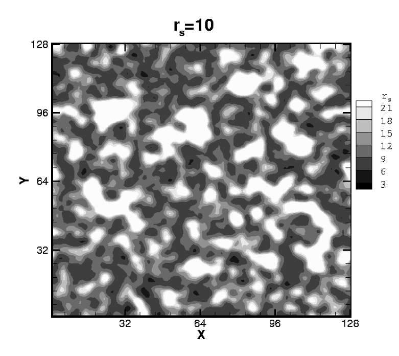
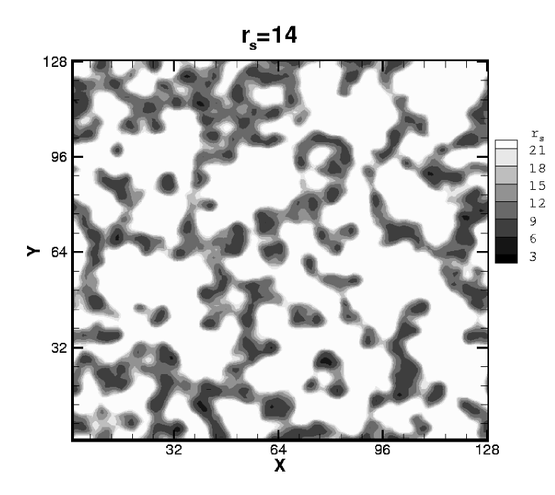
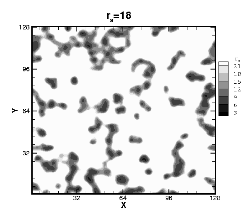
FIG. 1.: The density distributions for the different electron densities. We use the contour plot for the local density parameter $r_{s}=1/\sqrt{\pi n}$. The density of the white area decreases rapidly to zero. We take $V_{s}=0.2Ry^{*}$, $\xi=0.2L$.

Figure 1 shows the density distribution of the system. It can be clearly seen that the electrons form some high density regions, while the density of other regions are essentially zero. Depending on the average density of the system, the high density regions may connect each other together ($r_{s}=10$), or form some isolated regions ($r_{s}=18$). There exists a certain density ($r_{s}=14$) where the high density regions starts to percolate through the system, and form a conducting channel. The calculation clearly demonstrates the idea of our earlier theory [9], i.e., the metal-insulator transition observed in the 2D electron systems is the percolation transition of the electron density.

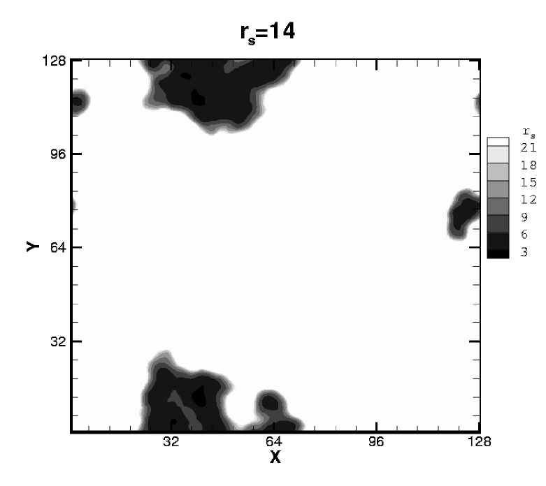
FIG. 2.: The density distribution for the free electron gas on the same disorder landscape as the Fig.1 at density $r_{s}=14$.

The electron-electron interaction is important for the conducting behavior of a dilute electron system in the sense that it makes the density distribution more extended because of the Coulomb repulsion. Figure 2 shows the density distribution for the free electron gas with the same density as in Fig.1(b) by turning off the electron-electron interaction. The system only forms some isolated high density regions at the disorder valleys, while the density distribution of the corresponding interacting system (Fig.1(b)) is quite extensive at the same density. At a given disorder strength, the critical density for the free electron gas is much higher than its interacting counterpart.

FIG. 3.: $\delta\mu/\delta N$ as a function of the electron density. Solid lines are for the uniform electron gas, squares are the data points for the disordered system, and the dashed-lines are the results from the theory discussed in the text. Two kinds of the disorder are used in the calculation: (a) The same disorder landscape as in Figure 1; (b) Off-plane charge impurities with $d=10a_{B}^{*}$, $n_{i}=2.5\times 10^{-3}/a_{B}^{*2}$. The parameters in the dashed-lines: (a) $n_{0}=10^{-3}/a_{B}^{*2}$, $\alpha=1.5$; (b) $n_{0}=0.5\times 10^{-3}/a_{B}^{*2}$, $\alpha=2.3$. $N$ is the total number of the electrons in the simulation box. $N=30$ corresponds to $r_{s}=18$; $N=50$ corresponds to $r_{s}=14$; $N=100$ corresponds to $r_{s}=10$.

Figure 3 shows the compressibility of the systems. To compare with the experiments[4, 6], we calculate $\delta\mu/\delta N$, which is the direct measured quantity in the experiments. It is well known that the compressibility of a uniform electron gas is negative in the low density region due to the effect of the exchange and correlation energies, as shown by the solid line in Fig.3(a). However, when the disorder is present, the behavior changes greatly. In the low density, the electrons tend to occupy the valleys of the disorder landscape, and the local density, instead of the average density, determines the compressibility of the system. On the other hand, at higher densities, all of the valleys are filled, one can expect the compressibility of the system to resume the behavior of a uniform electron gas. We have a non-monotonic behavior for $\delta\mu/\delta N$, as shown by the dots in Fig.3(a), which are in good agreement with the experimental measurement [4, 6]. Comparing with Fig.1, we find that the turning point of the compressibility ($N\approx 50$, $r_{s}\approx 14$) coincides with the percolation threshold of the system. At low densities, the data points in the plot show strong fluctuation, indicating the effect of the local fluctuation of the disorder potential.

The behavior can be understood by a simple theory. Following the definition, the chemical potential $\mu$ is the energy needed to add an electron into the system,

$$\mu(N) = E(N+1)-E(N)$$

$$\approx \varepsilon_{0}\left[n_{eff}(N+1)\right](N+1)-\varepsilon_{0}\left[n_{eff}(N)\right]N$$

$$= \frac{\delta}{\delta N}\left\{\varepsilon_{0}\left[n_{eff}(N)\right]N\right\},$$

where we suppose that the electron energy is determined by the local density of the electrons. $E(N)$ is the total energy of the system, $\varepsilon_{0}(n)$ is the energy per electron for the uniform electron gas, and $n_{eff}$ is effective local density. For the inhomogeneous system as shown in Fig.1, the effective local density can be estimated by $n_{eff}(n)\approx n/f(n)$, where $f(n)$ is the fraction of the high density region. After some algebra, we have

$$\mu(n) = \mu_{0}\left(\frac{n}{f}\right)\left[1-\frac{d\ln f}{d\ln n}\right]+\varepsilon_{0}\left(\frac{n}{f}\right)\frac{d\ln f}{d\ln n},$$

$$\frac{\delta\mu}{\delta n} = \mu_{0}^{\prime}\left(\frac{n}{f}\right)\frac{1}{f}\left[1-\frac{d\ln f}{d\ln n}\right]^{2}-\varepsilon_{0}^{\prime}\left(\frac{n}{f}\right)\left(\frac{n}{f}\right)^{2}\frac{d^{2}f}{dn^{2}}\,,$$

where $\mu_{0}$ is the chemical potential for a uniform electron gas. In the low density limit, $f(n)\rightarrow 0$, the local effective density is greatly different from the average density of the system. As a consequence, the density dependence of the chemical potential, $\delta\mu/\delta n$, changes greatly. In general, supposing $f(n)\sim n^{\alpha}$ in the low density limit, the analysis shows that $\delta\mu/\delta n$ will have a non-monotonic behavior if $\alpha>1$. The behavior of $f(n)$ is determined by the local disorder potential profile. In a 2D system, the infinite harmonic potential has $f(n)\sim n$. So the requirement $\alpha>1$ is equivalent to the condition that the local disorder potential has a weaker confinement effect than the harmonic potential. The condition can be easily satisfied in a typical experimental system. For instance, the coulomb potential has $f(n)\sim n^{4}$. In Fig.3, we use the above equation for $\delta\mu/\delta n$ with the following relation of $f(n)$ to fit the data,

$$f(n)=\frac{1}{1+\left(\frac{n_{0}}{n}\right)^{\alpha}}\,.$$

This form has a correct behavior in the high density limit, $f\rightarrow 1$, and the low density behavior is controlled by $\alpha$. By carefully choosing the values for $\alpha$ and $n_{0}$, we obtain a good agreement with our numerical data as shown in the dashed line in Fig.3(a).

To demonstrate the effect of a different disorder potential, we use off-plane charge impurity potential in calculating Figure 3(b), i.e.,

$$V_{d}({\bf x})=-\sum_{i}\frac{1}{\sqrt{|{\bf x}-{\bf x}_{i}|^{2}+d^{2}}}\,,$$

where $d$ is the distance between the electron and the impurity planes, and the impurities are randomly distributed with a density $n_{i}$. This potential gives a similar density profile as shown in Figure 1. As expected, this form of potential has a larger value of $\alpha$ as given in the figure caption.

To conclude, we have studied the electron space distribution and the compressibility of disordered dilute 2D electron systems by using the local density approximation. Electron distribution confirms the formation of the droplet state that consists of high and low density regions. Our calculated compressibility is in good agreement with the experimentally observed behavior showing unexpected anomaly at low densities. The turning point of the compressibility happens around the percolation threshold. Our theory based on the droplet state provides a good understanding of the compressibility anomaly.

This work is supported by DOE.

REFERENCES

- [1] S. V. Kravchenko, G. V. Kravchenko, J. E. Furneaux, V. M. Pudalov, and M. D’Iorio, Phys. Rev. B50, 8039 (1994); S. V. Kravchenko, W. E. Mason, G. E. Bowker, J. E. Furneaux, V. M. Pudalov, and M. D’Iorio, Phys. Rev. B51, 7038 (1995); S. V. Kravchenko, D. Simonian, M. P. Sarachik, W. Mason, and J. E. Furneaux, Phys. Rev. Lett. 77, 4938 (1996).
- [2] E. Abrahams, P.W. Anderson, D.C. Licciardello, and T.V. Ramakrishnan, Phys. Rev. Lett. 42, 673 (1979).
- [3] For a review, see E. Abrahams, S.V. Kravchenko, and M.P. Sarachik, cond-mat/0006055, and references therein.
- [4] C. Dultz and H.W. Jiang, Phys. Rev. Lett. 84, 4689 (2000).
- [5] S. Ilani, A. Yacoby, D. Mahalu, and H. Shtrikman, Phys. Rev. Lett. 84, 3133 (2000).
- [6] J.P. Eisenstein, L.N. Pfeiffer, and K.W. West, Phys. Rev. Lett. 68, 674 (1992); J.P. Eisenstein, L.N. Pfeiffer, and K.W. West, Phys. Rev. B50, 1760 (1994).
- [7] Q. Si and C.M. Varma, Phys. Rev. Lett. 81, 4951 (1998).
- [8] A.A. Pastor and V. Dobrosavljevic, Phys. Rev. Lett. 83, 4642 (1999).
- [9] S. He and X.C. Xie, Phys. Rev. Lett. 80, 3324 (1998); J. Shi, S. He and X.C. Xie, Phys. Rev. B60, R13950 (1999).
- [10] B. Tanatar and D.M. Ceperley, Phys. Rev. B39, 5005 (1989); S.T. Chui and B. Tanatar, Phys. Rev. Lett. 74, 458 (1995).
- [11] Y. Wang, J. Wang, H. Guo and E. Zarembar, Phys. Rev. B52, 2738 (1995), and references therein.