Ground-State Magnetization for Interacting Fermions in a Disordered Potential : Kinetic Energy, Exchange Interaction and Off-Diagonal Fluctuations

Abstract

We study a model of $n$ interacting fermions in a disordered potential, which is assumed to generate uniformly fluctuating interaction matrix elements. We show that the ground state magnetization is systematically decreased by off-diagonal fluctuations of the interaction matrix elements. This effect is neglected in the Stoner picture of itinerant ferromagnetism in which the ground-state magnetization is simply determined by the balance between ferromagnetic exchange and kinetic energy, and increasing the interaction strength always favors ferromagnetism. The physical origin of the demagnetizing effect of interaction fluctuations is the larger number $K$ of final states available for interaction-induced scattering in the lower spin sectors of the Hilbert space. We analyze the energetic role played by these fluctuations in the limits of small and large interaction $U$. In the small $U$ limit we do second-order perturbation theory and identify explicitly transitions which are allowed for minimal spin and forbidden for higher spin. These transitions then on average lower the energy of the minimal spin ground state with respect to higher spin; we analytically evaluate the size of this reduction and find it to give a contribution $\Delta^{s}\propto nU^{2}/\Delta$ to the spin gap between the two lowest spin ground-states. In term of an average effective Hamiltonian, these contributions induce a $nU^{2}S^{2}/\Delta$ term which decreases the strength of the ferromagnetic exchange, thereby delaying the onset of Stoner ferromagnetism, and generate a second, larger $S$ term $\propto S^{3}$ which results in a saturation of the ground-state spin before full polarization is achieved, in contrast to the Stoner scenario. For large interactions $U$ we amplify on our earlier work [Phys. Rev. Lett. 84, 3938 (2000)] which showed that the broadening of the many-body density of states is proportional to $\sqrt{K}U$ and hence favors minimal spin. Numerical results are presented in both limits. After evaluating the effect of fluctuations, we discuss the competition between fluctuations plus kinetic energy and the exchange energy. We finally present numerical results for specific microscopic models and relate them to our generic model of fluctuations. We discuss the different physical situations to which such models may correspond, the importance of interaction fluctuations, and hence the relevance of our results to these situations and recall an experimental setup which we proposed in an earlier work [2] to measure the importance of interaction fluctuations on the ground-state spin of lateral quantum dots in the Coulomb blockade regime.

I Introduction

A Stoner effect and disorder

More than fifty years ago Stoner proposed a simple route to ferromagnetism in itinerant systems based on the competition between one-body and interaction (exchange) energy [3]. The repulsive interaction energy can be minimized when the fermionic antisymmetry requirement is satisfied by the spatial wavefunction, as the overlap between different wavefunctions is then minimal. This effect favors the alignment of spins and, if the interaction is sufficiently strong, results in a large ground-state spin magnetization. This mechanism is the primary origin of Hund’s first rule in atomic physics. In contrast, when the interaction is weak minimal spin is favored, since in order to align spins electrons must be promoted from lower, doubly-occupied levels to higher singly-occupied levels and the cost in one-body energy is prohibitive. Because the Pauli principle is essentially local, ferromagnetism in metals has been studied within models such as the Hubbard model [4, 5] which only retain the short-range part of the electronic interaction; the long-range part of the interaction being assumed to give spin-independent contributions to the ground-state energy (the capacitance or charging energy). In the case of a Hubbard interaction, only pairs of electrons of opposite spin interact. The number of such pairs is a monotonically decreasing function of the total magnetization $\sim[(n/2)^{2}-\sigma^{2}]$ where $n$ is the number of electrons and $\sigma$ the total spin [6]. On the other hand, as just noted, flipping a spin requires the promotion of an electron to a higher one-body level and in the case of a finite system with a discrete spectrum of average spacing $\Delta$, a magnetization $\sigma$ requires an energy $\sigma^{2}\Delta$. A simple first order perturbation treatment shows then that a sufficiently strong interaction results in a finite magnetization, when the corresponding reduction in interaction energy counterbalances the increase in kinetic (one-body) energy

$$(\Delta-V_{c})\sigma^{2}=0$$ (1)

This occurs when the typical exchange interaction $V_{c}$ between two states close to the Fermi energy is equal to the one-particle level spacing which for a Hubbard interaction $U(\vec{r},\vec{r}^{\prime})=U\delta(\vec{r}-\vec{r}^{\prime})$ reads

$$V_{c}=U_{c}\int d\vec{r}\overline{|\psi_{\alpha}(\vec{r})|^{2}|\psi_{\beta}(\vec{r})|^{2}}=\Delta$$ (2)

The upper bar indicates an average over wavefunctions in the vicinity of the Fermi level. In a clean system this gives $U_{c}=\Delta$ and this threshold is known as the Stoner instability. As both the kinetic energy and the interaction energy have the same parametric dependence on the magnetization $\sigma$, reaching this threshold results in a second order phase transition to a ferromagnetic phase, the divergence of the magnetic susceptibility, and a macroscopic magnetization.

Quite naturally one may wonder in what way does the presence of a disordered potential modify this Stoner picture, and this question has recently attracted a lot of attention, both in the context of bulk metals (i.e. infinitely extended systems with diffusive eigenstates) and in finite-sized metallic systems such as quantum dots and metallic nanoparticles. Two types of questions have been considered: 1) The effect of a disordered potential on the average threshold for the Stoner instability. 2) The statistical properties of the threshold in an ensemble of mesoscopic metallic samples. Both aspects have been recently investigated theoretically. For the bulk case, it has been known for some time [7] that within perturbation theory disorder enhances the exchange effect in the susceptibility; recently Andreev and Kamenev constructed a mean-field theory which they argue describes the Stoner transition [8] and found a significant reduction of the Stoner threshold in low-dimensional disordered systems due to correlations in diffusive wavefunctions which enhance the average exchange term. In the framework of the same mean-field approach which neglects the fluctuations of the interactions, but takes into account those of the one-body spectrum, Kurland, Aleiner and Altshuler proposed that below, but in the immediate vicinity of the Stoner instability, there is a broad distribution of magnetization and that each sample’s free energy is characterized by a large number of local magnetization minima [14]. Brouwer, Oreg and Halperin [9] considered the effect of mesoscopic wavefunction fluctuations on the exchange interaction and found that their effect was to increase substantially the probability of non-zero spin magnetization in the ground state before the Stoner threshold is reached. Baranger, Ullmo and Glazman [10] suggested that the observed ”kinks” in the parametric variations of Coulomb blockade peak positions (e.g. as one varies an external magnetic field) could reflect changes in the ground state spin of the quantum dot. It was noted that the statistical occurence of nonzero ground-state magnetizations can account for the absence of bimodality of the conductance peak spacings distribution for tunneling experiments with quantum dots in the Coulomb blockade regime [11, 12, 13]. Another aspect of large disordered metallic samples is that the Stoner threshold can be locally exceeded, while the exchange averaged over the full sample has a value well below the threshold. In this case one may expect that localized regions with nonzero magnetization will be formed even though the full system is nonmagnetic. This scenario has been investigated by Narozhny, Aleiner and Larkin [15] who also considered the effect of such local spin droplets on dephasing. They found that the probability to form a local spin droplet though exponentially small, does not rigorously vanish as it would in a clean system, and that neither this probability, nor the corresponding spin depends on the droplet’s size. In a different approach focusing on the large interaction regime close to half-filling, Eisenberg and Berkovits numerically found that the presence of disorder may stabilize Nagaoka-like ferromagnetic phases at larger number of holes ($\geq 2$) [16]. Finally, Stopa has suggested that scarring of one-body wavefunctions in a chaotic confining potential may lead to strong enhancements of the exchange interaction and to the occurence of few-electron polarization in finite-sized systems [17]. Thus the general message of these works is that disorder tends to favor novel magnetic states over paramagnetic states.

B Overview and outline

In a recent letter [2], we pointed out a competing effect of interactions in disordered systems which reduces the probability of ground-state magnetization and hence favors paramagnetism. This effect had not (to our knowledge) been treated in any of the previous works on itinerant magnetization of disordered systems. The works cited above neglect the effect of disorder in inducing fluctuations in the off-diagonal interaction matrix elements [8, 14]. However it is well-known from studies of complex few-body systems like nuclei and atoms [18, 19] that the band-width of the many-body density of states in finite interacting fermi systems is strongly modified by the fluctuations of these off-diagonal matrix elements already at moderate strength of the interactions. Such studies did not directly address the effect of this broadening on the ground-state spin of the system. However our extension of these models immediately revealed that these fluctuations are largest for the states of minimal spin, due to the larger number of final states (non-zero interaction matrix elements) for interaction-induced transitions (we will review this argument below). This effect then significantly increases the probability that the extremal (low-energy) states in the band are those of minimal spin and opposes the exchange effect. In our earlier works [2, 20] we focused on the regime of large fluctuations to deduce the scaling properties of the ground-state energy as a function of spin, and verified these scaling laws with numerical tests. In the present work we will review and extend these results for large fluctuations, but we will focus mostly on the perturbative regime of small $U$. While in this regime the correction to the ground-state energy due to fluctuations is small by assumption, one is able to evaluate these corrections analytically and show that they favor minimal spin for an arbitrary number of particles. Specifically, the larger number of interaction-induced transitions for lower spin leads to more and larger interaction contributions to the (negative) second-order correction to the ground-state energy in each spin block. This illustrates explicitly the ”phase-space” argument introduced in [2, 20] which implies that fluctuations generically suppress magnetization. We expect this effect to be significant in quantum dots where it will reduce the probability of high spin ground states. We recall that the ground state spin of lateral quantum dots can be experimentally determined by following the motion of Coulomb blockade conductance peaks as an in-plane magnetic field is applied [2]. Therefore the strength of the demagnetizing effect of fluctuations of interaction is experimentally accessible.

The paper is organized as follows. In section II we start by an explicit derivation of our model and describe its main features. In section III we begin for pedagogical reasons with an analytical treatment of the model for the case of only two particles, in both the perturbative regime of weak off-diagonal fluctuations and the asymptotic regime where they dominate. Section IV will be devoted to a second order perturbative treatment of the model for an arbitrary number of particles; this will be followed in section V by a discussion of the magnetization properties of the system’s ground state in the asymptotic regime. As noted above, some of the results presented there have already been presented in [2, 20] but are nevertheless included to make the article self-contained. In the next section VI we consider the competition between exchange and fluctuations in more details, both from the point of view of average Stoner threshold and in terms of probability of finding a polarized ground-state. We will see in particular that the off-diagonal fluctuations induce a term $\sim\sigma^{2}$ in the Hamiltonian which delays the Stoner instability and a second term $\sim\sigma^{3}$ which strongly suppresses the occurence of large ground-state spins even above the Stoner instability. In section VII we consider more standard microscopic models for disordered interacting fermions and relate their properties to our generic model of fluctuating interactions. We determine the conditions to be satisfied in order for the results obtained from our random interaction model to be relevant in different physical situations. Finally we summarize our findings, put them in perspective and discuss possible extensions of this work in the final section VIII.

II Derivation of the Model

Our starting point is a lattice model for fermions in a disordered potential coupled by a two-body, spin-independent interaction of arbitrary range. We make a unitary transformation to the basis of single-particle eigenstates of the disordered potential and introduce the assumption that the single-particle states are random and uncorrelated. Upon averaging over disorder we arrive at a completely generic model describing both the nonvanishing average interactions (exchange,charging and BCS) and the statistical fluctuations in both the one and two-body terms. Finally we introduce the assumption that all interaction matrix elements have the same statistical variance. Hence our construction excludes both one-body integrable systems and strongly-localized systems. We also note that with this assumption geometric or commensurability effects (such as spin waves or antiferromagnetic instabilities) cannot be captured by our treatment, as the statistical character of the construction erases most real-space details of the model.

We consider the following tight-binding Hamiltonian for $n$ spin-$1/2$ particles

$${\cal H} = {\cal H}_{0}+{\cal U}=\sum_{i,j;s}{\cal H}_{0}^{i,j}d^{\dagger}_{i,s}d_{j,s}+\sum_{i\neq j}{\cal U}(i-j)n_{i}n_{j}+\sum_{i}{\cal U}(0)n_{i,\uparrow}n_{i,\downarrow}$$ (3)

$s=\uparrow,\downarrow$ is a spin index, $d^{\dagger}_{i,s}$ ($d_{i,s}$) creates (destroys) a fermion on the i^th site of a $D$-dimensional lattice of linear dimension $La$ and volume $\Omega=(La)^{D}$. This latter quantity defines the number $m/2=\Omega/a^{D}$ of spin-degenerate one-body eigenenergies which we will refer to as orbitals in what follows, $a\equiv 1$ is the lattice constant. ${\cal H}_{0}$ is a one-body, spin independent, disordered Hamiltonian with eigenvalues $\epsilon_{\alpha}$ and eigenvectors $\psi_{\alpha}$, i.e. one has

$${\cal H}_{0}|\psi_{\alpha}\rangle=\epsilon_{\alpha}|\psi_{\alpha}\rangle=\epsilon_{\alpha}\sum_{i}\psi_{\alpha}(i)|i\rangle$$ (4)

where $|i\rangle$ refers to a lattice site ket.

We assume that ${\cal H}_{0}$ has no degeneracy besides twofold spin-degeneracy and distribute the $m/2$ different one-body energies as $\epsilon_{\alpha}\in[0;m/2]$ so as to fix $\Delta\equiv 1$ without spin degeneracy. Below we will discuss three different eigenvalue distributions : constant spacing distribution [21] ($\epsilon_{\alpha}=(\alpha-1)\Delta$, note that due to the level degeneracy the single-particle level spacing is $\Delta$, whereas $\Delta/2$ is the mean level spacing), randomly distributed $\epsilon_{\alpha}$ with a Poisson spacing distribution, or with a Wigner-Dyson spacing distribution. Finally ${\cal U}(i-j)$ is the electron-electron interaction potential and $n_{i}=\sum_{s}n_{i,s}=\sum_{s}d^{\dagger}_{i,s}d_{i,s}$. The Hamiltonian is Spin Rotational Symmetric (SRS) so that both the total spin $|\vec{S}|$ and its projection $S_{z}$ commute with the Hamiltonian and the corresponding eigenvalues $\sigma$ and $\sigma_{z}$ are good quantum numbers. This results in a block structure of the Hamiltonian ${\cal H}$ which will be described in detail below. Performing the unitary transformation defined by

$$\sum_{\alpha}\psi_{\alpha}(i)c^{\dagger}_{\alpha,s} = d^{\dagger}_{i,s},$$ (5)

we rewrite the Hamiltonian as

$${\cal H} = \sum\epsilon_{\alpha}c^{\dagger}_{\alpha,s}c_{\alpha,s}+\sum U_{\alpha,\beta}^{\gamma,\delta}c^{\dagger}_{\alpha,s}c^{\dagger}_{\beta,s^{\prime}}c_{\delta,s^{\prime}}c_{\gamma,s}$$ (6)

where the Interaction Matrix Elements (IME) are given by

$$U_{\alpha,\beta}^{\gamma,\delta} = \sum_{i,j}{\cal U}(i-j)\psi_{\alpha}^{*}(i)\psi_{\beta}^{*}(j)\psi_{\delta}(j)\psi_{\gamma}(i)$$ (7)

These IME induce transitions between many-body states differing by at most two one-body occupation numbers. The distribution and properties of the IME depend on both the range of the interaction potential and the one-particle dynamics. If there are conserved quantities other than energy in the one-particle dynamics (and hence good quantum numbers describing the one-body states) this will lead to selection rules in the IME; the extreme case of this would be an integrable one-particle hamiltonian for which a complete set of quantum numbers exists. Selection rules greatly reduce the number of allowed interaction-induced transitions, and lead to a very singular distribution of IME (this is most easily seen by considering a clean hypercubic lattice model with Hubbard interaction). Perturbing a clean lattice with a disordered potential destroys translational symmetry and these selection rules disappear, which induces a crossover of the distribution of IME from a set of $\delta-$functions to a smooth distribution. In Fig.24 we illustrate this by plotting the distribution of IME for a one-dimensional lattice model with on-site disorder, nearest and next-nearest-neighbor hopping and a Hubbard interaction as described e.g. in reference [22].

The key assumption of our model is that such a smooth distribution of interaction matrix elements exists and that in fact all matrix elements which preserve SRS have the same nonzero variance (these matrix elements may vanish on average of course). This assumption rules out both the case of integrable one-body dynamics as discussed above, and the case of strongly-localized wavefunctions for which interaction matrix elements between states separated spatially by more than a localization length will have different (and much smaller) variance than those in the same localization volume. Our assumption is reasonable for metallic disordered states with a randomness generated by either impurities or chaotic boundary scattering.

With this motivation, we assume that the fluctuations of the off-diagonal $U_{\alpha,\beta}^{\gamma,\delta}$ are random with a zero-centered gaussian distribution of width $U$. Only matrix elements $U_{\alpha,\beta}^{\alpha,\beta}$, $U_{\alpha,\beta}^{\beta,\alpha}$ and $U_{\alpha,\alpha}^{\beta,\beta}$ have nonzero averages $\langle U_{\alpha,\beta}^{\alpha,\beta}\rangle$, $\langle U_{\alpha,\beta}^{\beta,\alpha}\rangle$ and $\langle U_{\alpha,\alpha}^{\beta,\beta}\rangle$ which lead (respectively) to mean-field charge-charge, spin-spin and BCS-like interaction terms. Note that the average of both the exchange and BCS terms is dominated by the short-range part of the interaction, and that ${\cal U}_{BCS}$ vanishes as time-reversal symmetry is broken. Consequently, the electronic interactions give us four contributions. The first three are the average charge-charge, ferromagnetic spin-spin and BCS terms that we just discussed and which can be written as ($n_{\alpha}=\sum_{\alpha,s}c^{\dagger}_{\alpha,s}c_{\alpha,s}$ and $n=\sum_{\alpha}n_{\alpha}$.)

$${\cal U}_{avg} = {\cal U}_{cc}+{\cal U}_{ss}+{\cal U}_{BCS}=\left[\langle U_{\alpha,\beta}^{\alpha,\beta}\rangle-\frac{1}{2}\langle U_{\alpha,\beta}^{\beta,\alpha}\rangle\right]n(n+1)/2-\lambda U\vec{S}\cdot\vec{S}+\sum_{\alpha,\beta}\langle U_{\alpha,\alpha}^{\beta,\beta}\rangle c^{\dagger}_{\alpha,\uparrow}c^{\dagger}_{\alpha,\downarrow}c_{\beta,\downarrow}c_{\beta,\uparrow}$$ (8)

where we have introduced spin operators $\vec{S}_{\alpha}\equiv(1/2)\sum_{s,t}c^{\dagger}_{\alpha,s}\vec{\sigma}_{s,t}c_{\alpha,t}$ and $\vec{S}=\sum_{\alpha}\vec{S}_{\alpha}$. Note that the strength of the average ferromagnetic exchange term has been written in units of the rms fluctuation $U$, i.e. we have introduced a parameter $\lambda$ which is the ratio of the average exchange to the fluctuations

$$\lambda\equiv 2\langle U_{\alpha,\beta}^{\beta,\alpha}\rangle/U$$ (9)

much in the same spirit as the usual Stoner picture where another energy ratio $\langle U_{\alpha,\beta}^{\beta,\alpha}\rangle/\Delta$, between the exchange energy and the one-body energy spacing at the Fermi level, is the relevant parameter.

The fourth interaction contribution to our model hamiltonian goes beyond the mean-field approximation and contains the off-diagonal fluctuations of the electronic interactions

$${\cal U}_{f} = \sum_{\alpha,\beta;\gamma,\delta}\sum_{s,s^{\prime}}\bar{U}_{\alpha,\beta}^{\gamma,\delta}c^{\dagger}_{\alpha,s}c^{\dagger}_{\beta,s^{\prime}}c_{\delta,s^{\prime}}c_{\gamma,s}$$ (10)

Having removed the average interactions, we now assume that both the diagonal and off-diagonal IME $\bar{U}_{\alpha,\beta}^{\gamma,\delta}$ have zero-centered uncorrelated gaussian distributions $P(\bar{U}_{\alpha,\beta}^{\gamma,\delta})\propto e^{-(\bar{U}_{\alpha,\beta}^{\gamma,\delta})^{2}/2U^{2}}$ of width $U$. We stress that in general, not all IME have the same variance but being interested in generic features of the interaction, we will neglect these variance discrepancies. ${\cal U}_{f}$ contains three kind of matrix elements, the variances of which depend on the number of transferred one-body occupancies between the connected Slater determinants. Diagonal matrix elements ${\cal U}_{f}^{I,I}=\langle I|{\cal U}_{f}|I\rangle$ ($|I\rangle$ denotes a Slater determinant) have a variance $\sim n(n-1)U^{2}/2$, one-body off-diagonal elements that change only one occupancy have a variance $\sim(n-1)U^{2}$ whereas generic two-body off-diagonal matrix elements inducing transitions between Slater determinants differing by exactly two occupancies, have the generic variance $U^{2}$. In diagrammatic language, these discrepancies occur due to the presence of up to two closed loops in the diagram corresponding to these matrix elements, each loop corresponding to a sum over $O(n)$ uncorrelated IME.

Our full Hamiltonian then reads

$${\cal H} = {\cal H}_{0}+{\cal U}_{avg}+{\cal U}_{f}$$ (11)

The mean-field Hamiltonian proposed in [14] was constructed along similar lines but neglects the fluctuations of interaction ${\cal U}_{f}$ and is thus embedded in the above Hamiltonian (11). Consequently, all results derived there can be obtained from the treatment to be presented below after setting the strength of fluctuations $U\rightarrow 0$. In a condensed matter context this is justified in the limit of large conductance $g\rightarrow\infty$. As recent experiments in quantum dots seem to be consistant with a conductance $g\approx 6-8$ [12], it is a priori not obvious that ${\cal U}_{f}$ can be neglected. We also stress that both the Random Matrix Theory (RMT) symmetry under orthogonal (or unitary) basis transformation in the one-body Hilbert space (which in metallic samples is satisfied for energy scales smaller than the Thouless energy $E_{c}=g\Delta$ [41]), and the $SU(2)$ symmetry under rotation in spin space are satisfied by each of the three terms in the above Hamiltonian.

The charge-charge mean-field contribution results in a constant energy shift of the full spectrum and has thus no influence on the ground-state spin; we therefore neglect it henceforth. This must however be kept in mind, as it is for instance well known that including self-consistently the mean-field charge-charge contribution of the interactions (e.g. in a Hartree-Fock approach) leads to significant corrections to the one-particle density of states at the Fermi level [7, 23, 24]. The BCS term gives rise to superconducting fluctuations for a negative effective interaction in the Cooper channel $\langle U_{\alpha,\alpha}^{\beta,\beta}\rangle<0$. We shall only consider disordered metallic samples which have $\langle U_{\alpha,\alpha}^{\beta,\beta}\rangle>0$. In this case the renormalization group flow brings the BCS coupling to zero [25]. We thus also neglect this term and set ${\cal U}_{avg}={\cal U}_{ss}$. Note however that the presence of a nonzero (repulsive or attractive) BCS coupling may stabilize a paramagnetic phase.

After these considerations we reach our model Hamiltonian

$${\cal H} = \sum_{\alpha}\epsilon_{\alpha}n_{\alpha}-\lambda U\vec{S}\cdot\vec{S}+\sum_{\alpha,\beta;\gamma,\delta}\sum_{s,s^{\prime}}\bar{U}_{\alpha,\beta}^{\gamma,\delta}c^{\dagger}_{\alpha,s}c^{\dagger}_{\beta,s^{\prime}}c_{\delta,s^{\prime}}c_{\gamma,s}$$ (12)

Due to the SRS that we imposed on the original Hamiltonian (3), the interaction commutes with the total magnetization $|\vec{S}|^{2}$ and its projection $S_{z}$ so that the Hamiltonian acquires a block structure where blocks are labelled by a quantum number $\sigma_{z}$ and subblocks of given $\sigma\geq\left|\sigma_{z}\right|$ appear within each of these blocks. Each block’s size is given in term of binomial coefficients as $N(\sigma_{z})=\left({}_{n/2-\sigma_{z}}^{m/2}\right)\left({}_{n/2+\sigma_{z}}^{m/2}\right)$, while the size of a subblock of given $\sigma$ is given by $N(\sigma)=N(\sigma_{z}=\sigma)-N(\sigma_{z}=\sigma+1)$. Due to SRS it is sufficient to study the block with lowest projection $\sigma_{z}=0$ $(1/2)$ for even (odd) number of particles, as all values of $\sigma$ will be included in this block. For simplicity, we will consider an even number $n$ of particles in the initial discussion presented below, and will generalize the discussion later on to include odd $n$, highlighting the main differences between the two cases. It is important to remark that both $\sigma$ and $\sigma_{z}$ are not only good quantum numbers for the full Hamiltonian, but also individually for ${\cal H}_{0}$, ${\cal U}_{avg}$ and ${\cal U}_{f}$. This allows us to consider each of these terms separately and in the next two chapters we will make use of this property, first neglecting ${\cal U}_{ss}$ : as it only generates constant energy shifts within each sector, it can be added after the restricted problem ${\cal H}_{0}+{\cal U}_{f}$ has been solved.

In (10) the sums in both the spin and orbital indices are not restricted, i.e $s,s^{\prime}=\downarrow,\uparrow$ and $\alpha,\beta,\gamma,\delta=1,2,...m/2$. It is both convenient and instructive to rewrite it as

$${\cal U}_{f} = \sum_{\alpha>\beta;\gamma<\delta}\sum_{s_{z}=0,\pm 1}V_{\alpha,\beta}^{\gamma,\delta}T^{\dagger}_{\alpha,\beta}(s_{z})T_{\gamma,\delta}(s_{z})+\frac{1}{2}\sum_{\alpha\geq\beta;\gamma\leq\delta}W_{\alpha,\beta}^{\gamma,\delta}S^{\dagger}_{\alpha,\beta}S_{\gamma,\delta}(1-\frac{1}{2}\delta_{\alpha,\beta})(1-\frac{1}{2}\delta_{\gamma,\delta})$$ (13)

where we have introduced totally symmetric and antisymmetric matrix elements

$$W_{\alpha,\beta}^{\gamma,\delta} = \bar{U}_{\alpha,\beta}^{\gamma,\delta}+\bar{U}_{\beta,\alpha}^{\delta,\gamma}+\bar{U}_{\alpha,\beta}^{\delta,\gamma}+\bar{U}_{\beta,\alpha}^{\gamma,\delta}$$ (14)

$$V_{\alpha,\beta}^{\gamma,\delta} = \bar{U}_{\alpha,\beta}^{\gamma,\delta}+\bar{U}_{\beta,\alpha}^{\delta,\gamma}-\bar{U}_{\alpha,\beta}^{\delta,\gamma}-\bar{U}_{\beta,\alpha}^{\gamma,\delta}$$ (15)

as well as two-body creation and destruction operators for either singlet-paired

$$S^{\dagger}_{\alpha,\beta}=(c^{\dagger}_{\alpha,\uparrow}c^{\dagger}_{\beta,\downarrow}-c^{\dagger}_{\alpha,\downarrow}c^{\dagger}_{\beta,\uparrow})/\sqrt{2}\ \ \ ;\ \ \ S^{\dagger}_{\alpha,\alpha}=c^{\dagger}_{\alpha,\uparrow}c^{\dagger}_{\alpha,\downarrow}$$ (16)

or triplet-paired fermions

$$T^{\dagger}_{\alpha,\beta}(0)=(c^{\dagger}_{\alpha,\uparrow}c^{\dagger}_{\beta,\downarrow}+c^{\dagger}_{\alpha,\downarrow}c^{\dagger}_{\beta,\uparrow})/\sqrt{2}\ \ \ ;\ \ \ T^{\dagger}_{\alpha,\beta}(s)=c^{\dagger}_{\alpha,s}c^{\dagger}_{\beta,s}\ \ ,\ \ s=\uparrow,\downarrow$$ (17)

As we consider fully uncorrelated IME $U_{\alpha,\beta}^{\gamma,\delta}$, both the symmetrized and antisymmetrized matrix elements have the same variance which for no doubly appearing indices reads

$$\sigma^{2}\left(W_{\alpha,\beta}^{\gamma,\delta}\right)=\sigma^{2}\left(V_{\alpha,\beta}^{\gamma,\delta}\right)=4U^{2}$$ (18)

In principle, the ratio of the variances strongly depends on microscopic details, in particular the range of the interaction. For instance, it can easily be seen that $\sigma^{2}\left(V_{\alpha,\beta}^{\gamma,\delta}\right)/\sigma^{2}\left(W_{\alpha,\beta}^{\gamma,\delta}\right)\in[0,1]$ and that the ratio vanishes for a Hubbard interaction. We will neglect this discrepancy however, but note that an increased variance of the symmetrized IME with respect to the antisymmetrized ones favors a low spin ground-state [26].

The hamiltonian can now be regarded as acting on singlet or triplet bonds between levels. SRS is then reflected in the simple statement that the destruction of a bond between two fermions must be followed by the re-creation of a bond of the same nature. We note that the triplet operators (17) create either a $\sigma_{z}=0$, $\sigma=1$ or a $\sigma_{z}=\pm 1$, $\sigma=1$ two-fermion state in a fixed spin basis. A rotation in spin space would bring the operators in (17) into one another and the first three terms in the brackets in (13) are not individually SRS but must be considered as one single spin-conserving operator. We illustrate this point in Appendix A, where we evaluate the effect of this operator acting on a four-particle state with two double occupancies. Note also that from (7) and (14), a purely on-site interaction influences only the singlet channel as in this case the antisymmetrized IME vanish identically.

The procedure leading to (13) amounts to a projection of the interaction operator onto the two irreducible representations of the two-fermion symmetry group. In this way the two-body singlet matrix elements are explicitly separated from their triplet counterparts, and the rewriting leading to (13) allows us to formulate the many-body problem in term of two-particles bonds of different nature in a similar way as the authors of [26]. Any even $n$-fermion state is represented as a $n/2$-boson state where each boson has either spin $\sigma=0$ or 1. These bosons can be constructed by acting on the vacuum $|0\rangle$ with an $S$ or a $T$ operator respectively, and the spin of these composite bosonic states depends on the bond between the two fermions, i.e. whether the fermionic antisymmetry is supported by the spin or the spatial degrees of freedom. Alternatively, this means that for a $n$-body state of total spin $\sigma$, the number of triplet bonds is given by $\sigma$ [27]. Also double orbital occupancies result in singlet bonds, so that their number is restricted to $[0,n/2-\sigma]$. This construction leads however to an overcomplete basis for $n\geq 6$. We were unable to propose a systematic reduction to an orthonormal set of states nor are we aware of any such systematic construction in the literature. For the computations to be carried below it will however be sufficient to know that such a basis can in principle be constructed (via e.g. reduction and orthogonalization of the constructed overcomplete basis), and how to construct it for the special case of four particles above the filled fermi sea, as those are the only states one encounters when doing second order perturbation theory for the levels of lowest energy in the $\sigma=0$ and 1 sectors.

Equation (13) helps us see the key qualitative point of our work. In second order perturbation theory ${\cal U}_{f}$ will generate transitions in each spin sub-block between the ground state and excited states differing by two occupation numbers (or less). Both the triplet and singlet terms will generate transitions, but there are certain types of transitions which can be generated by the singlet term which cannot be generated by the triplet term. For instance the triplet operator cannot generate transitions to final states with additional double occupancies nor is it possible to scatter a triplet bonded pair into a double occupancy (see Fig. 24). As the magnetization increases, the number of singlet transitions decreases accordingly as the number of singlet two-particle bonds in a many-body state obviously decreases with its total magnetization. Eventually, when $\sigma$ is maximal, only triplet transitions survive and we can readily conclude that the number of two-body transitions is a monotonically decreasing function of the magnetization as is therefore the number of (energy-decreasing) second order contributions. We will see below that this condition on the available volume for phase-space scattering is crucial for the ground-state magnetization properties, both in the perturbative regime ($U/\Delta\ll 1$) and in the asymptotic limit of dominant fluctuations ($U/\Delta\gg 1$). It is important to understand that the relevant variable here is the number of transitions and not the size of the Hilbert space; the block size $N(\sigma)$ is in general (for a sufficient number of particles) a nonmonotonic function of $\sigma$, as on one hand $N(\sigma=n/2)<N(\sigma=0)$ (or $N(\sigma=n/2)<N(\sigma=1/2)$ for odd number of particles), whereas on the other hand, and in the limit $\sigma\ll n/2\ll m/2$, it can be shown using Stirling’s formula that $\partial N(\sigma)/\partial\sigma>0$. Except for very few particles, $N(\sigma)$ has its maximum at a finite magnetization, whereas the number of transitions is always maximum for $\sigma=0$.

We close this introductory chapter with a brief historical survey of random interaction models similar to (12-13). These models originated in nuclear physics and are based on similar principles as those which led Wigner to propose the gaussian ensembles of random matrices, with the additional requirement that they represent particles interacting via a $k$-body interaction. Only when the rank $k$ of the interaction is equal to the number $n$ of particles does one recover the Wigner gaussian ensembles. Physically, interactions are in principle not random per se, however once one postulates the invariance of the one-body Hamiltonian matrix ensemble under unitary (i.e. basis) transformation, a postulate motivated e.g. by a chaotic one-body dynamics, random IME naturally appear (see (7)), and this results in a similar invariance for the many-body Hamiltonian ensemble and the associated probability distribution $P({\cal H})\propto\exp(-{\rm Tr}{\cal H}^{2}/2)$. The first proposed model with random interactions was the fermionic Two-Body Random Interaction Model (TBRIM) for spinless fermions which was introduced independently by French and Wong and Bohigas and Flores [28]. This model is essentially a spinless version of ${\cal U}_{f}$. While significant deviations from the usual gaussian ensemble of random matrices were found in the tails of the spectrum - in particular the MBDOS for $n\gg 2$ has a gaussian, not a semicircular shape - these authors found no significant differences in the spectral properties at high excitation energy. (This latter finding has been however challenged very recently [29] and may be due to the smallness of the systems considered.) More recently this spinless TBRIM was extended with a one-body part and it has been discovered that the critical interaction strength $U_{c}$ at which WD statistics sets in is governed by the energy spacings $\Delta_{c}$ between directly coupled states [30]. This model and similar ones have also been studied in the framework of quantum chaos in atomic physics [31], in particular the thermalization of few-body isolated systems has attracted a significant attention [32, 33], and more recently in solid-state physics to study quasiparticle lifetime [30, 36, 37, 38, 39, 40] and fluctuations of Coulomb blockade conductance peak spacings and heights in quantum dots [34, 35]. In a solid-state context however the invariance of the one-body Hamiltonian under basis transformation is satisfied only in an energy interval of the order of the Thouless energy $E_{c}=g\Delta$ around the Fermi energy, where $g$ is the conductance [41]. Wavefunctions correlations become stronger and stronger beyond the Thouless energy where IME start to decay algebraically as a function of the energy. It is thus reasonable to consider our random interaction model as an effective truncated Hamiltonian in an energy window given by the Thouless energy $E\in[E_{f}-E_{c},E_{F}+E_{c}]$ [36], so that the number of particles and orbitals behave as $m$,$n\sim g$. Nuclear shell models may also be represented by randomly interacting models, differing from the original TBRIM in the presence of additional quantum numbers like spin, isospin, parity and so forth[33]. Most of those models consider the limit of dominant fluctuations $U/\Delta\gg 1$ and quite unexpectedly, it has been found that even in this regime, random interactions may result in an orderly behavior [42], in particular a strong statistical bias toward a low angular momentum ground-state. In particular, for the special case of an angular momentum restricted to $j_{z}=\pm 1/2$, the probability of finding a zero angular momentum ground-state for an even number of nucleons reaches almost 100% [2, 26]. While the reasons for this behavior in the asymptotic regime are still not clear [43], we will see below that a strong bias toward low angular momentum ground-state results from a stronger broadening of the Many-Body Density of States (MBDOS) in the low spin sector, associated with a larger number of off-diagonal transitions. The same phenomenon with qualitatively the same origin will be shown to influence the ground-state magnetization in the perturbative limit.

III The Case of $n=2$ Fermions

For $n=2$ particles, only the sectors $\sigma=0$ and $1$ exist whose size is given by $N(\sigma)=m/2(m/2+1-2\sigma)/2$. In each sector, the interaction matrix ${\cal U}_{f}$ is a GOE matrix (the number of particles is equal to the rank of the interaction) and all Hamiltonian matrix elements are non-zero and have the same variance. For simplest case of two orbitals ($m/2=2$) one can demonstrate the magnetization reducing effect of interaction Fluctuations by an argument which is exact for all values of the off-diagonal fluctuations $U$. The two orbitals are spin-degenerate and have energies $\epsilon_{1}=0$ and $\epsilon_{2}=\Delta>0$. In the absence of interaction fluctuations, the three eigenvalues in the $\sigma=0$ sector are $0$, $\Delta$ and $2\Delta$. Switching on the interaction, the determinant of the Hamiltonian matrix in the time-reversal symmetric case can be written

$${\rm Det}{\cal H} = \frac{1}{2}W_{1,1}^{1,1}(\Delta+\frac{1}{2}W_{1,2}^{1,2})(2\Delta+\frac{1}{2}W_{2,2}^{2,2})+\frac{1}{4}W_{1,2}^{1,1}W_{2,2}^{1,2}W_{2,2}^{1,1}$$ (19)

$$- \frac{1}{4}\left[\frac{1}{2}W_{1,1}^{1,1}(W_{2,2}^{1,2})^{2}+(W_{1,2}^{1,1})^{2}(2\Delta+\frac{1}{2}W_{2,2}^{2,2})+(W_{2,2}^{1,1})^{2}(\Delta+\frac{1}{2}W_{1,2}^{1,2})\right]$$ (20)

Every single term in this expression has a symmetric distribution, i.e. an equal probability of being positive or negative, except for a term $-((W_{2,2}^{1,1})^{2}+2(W_{1,2}^{1,1})^{2})\Delta/4$ which is always negative. It results that the determinant has a higher probability of being negative which in its turn means that the lowest eigenvalue (which vanishes at $U/\Delta=0$) is statistically more often negative than positive when $U$ is switched on - it is more likely to be reduced than increased by the off-diagonal fluctuations. Simultaneously, and in absence of exchange, the energy of the only $\sigma=1$ level is given by $\Delta+V_{1,2}^{1,2}/2$, so that the fluctuations lower or increase it with equal probability. Hence fluctuations always increase the average spin gap in this case.

We next consider an arbitrary number of orbitals, $m$. First consider the limit of dominant fluctuations $U/\Delta\gg 1$. ${\cal H}\approx{\cal U}_{f}$ is then a GOE matrix and its MBDOS is well approximated by a semicircle law ($E^{2}\leq E_{0}^{2}$)

$$\rho_{GOE}=\frac{2}{\pi E_{0}^{2}(\sigma)}\sqrt{E_{0}^{2}(\sigma)-E^{2}}$$ (21)

where $E_{0}(\sigma)\approx\sqrt{2N(\sigma)}U$. This expression is not exact however as there are corrections in the tail of the distribution [44] as one can see on Fig. 24. These corrections behave as $O(N^{-1/6})$ while the level density there is $O(N^{1/6})$ [44], i.e. the number of levels outside the semicircle is independent of N (and hence of $m$) and for simplicity we will neglect these corrections in what follows.

Henceforth we shall be focusing attention on the ground state in each spin sector and the gaps between these ground states, so it is useful to adopt the standard term in nuclear physics for the lowest levels, of a given spin or angular momentum, yrast levels. In the current model, in the asymptotic regime of large fluctuations $U/\Delta\gg 1$, (and neglecting the exchange interaction) we can approximate the energy of the yrast states by $E_{0}(\sigma)$ and hence readily predict that the average $\sigma=0$ yrast energy will be lower than its $\sigma=1$ counterpart by an amount

$$\Delta^{s}\equiv\overline{{\cal E}_{0,\sigma=1}-{\cal E}_{0,\sigma=0}}\approx U(\sqrt{m(m/2+1)/2}-\sqrt{m(m/2-1)/2})=U+O(\frac{1}{m})$$ (22)

i.e. on average there is a spin gap for $U/\Delta\gg 1$ in the large $m$ limit. Next we can calculate the average energy of the first excited $\sigma=0$ level ${\cal E}_{1,\sigma=0}$ via integration of the average MBDOS (21) as

$$\overline{{\cal E}_{1,\sigma=0}-{\cal E}_{0,\sigma=0}}=O(N(\sigma)^{-1/6})=O(m^{-1/3})$$ (23)

In the relevant limit $m\gg 1$ the splitting between this first excited $\sigma=0$ level and the $\sigma=0$ yrast level is negligible and both states are below the $\sigma=1$ yrast level by a gap of order $U$, independent of $m$. This calculation can be extended to higher $\sigma=0$ excited states and the result suggests that on average there is a large number $O(m^{1/3})$ of $\sigma=0$ levels which have a lower energy than the first spin excited state. Remember however that we have neglected corrections to the tails of the density of states, and it turns out that these corrections result in an $m$-independent number $p\approx 3$ of $\sigma=0$ levels in the spin gap as shown by the numerical data presented in Fig. 24. In Fig. 24 we show a numerical check which confirm the validity of (22) up to prefactors which are due to additional correlations between the considered levels and cannot be captured by the simple arguments presented here. We will come back to this point in section V. Note however that the distance between ${\cal E}_{0,\sigma=0}$ and ${\cal E}_{1,\sigma=0}$ seem to remain constant as $m$ increases which is a manifestation of the presence of the tail correction to the semicircle law (21) and is beyond the reach of the simplified reasoning we have presented.

We can next calculate perturbatively the energy of the yrast state in each sector up to the second order in $U/\Delta$. These states can be written as (the singlet and triplet creation operators $S_{1,1}^{\dagger}$ and $T_{1,2}^{\dagger}(0)$ have been defined in (16) and (17))

$$|\Psi_{0}^{(\sigma=0)}\rangle = S_{1,1}^{\dagger}|0\rangle$$ (24)

$$|\Psi_{0}^{(\sigma=1)}\rangle = T_{1,2}^{\dagger}(0)|0\rangle$$ (25)

Up to the first order their energies are given by

$${\cal E}_{0,0} = 2\epsilon_{1}+W_{1,1}^{1,1}/2$$ (26)

$${\cal E}_{0,1} = \epsilon_{1}+\epsilon_{2}+V_{1,2}^{1,2}/2-2\lambda U$$ (27)

and the second order corrections read (using the constant spacing model for the one-particle levels)

$$\overline{\Delta{\cal E}_{0,0}^{(2)}} = -\frac{1}{2}\sum_{\alpha\geq\beta>2}\frac{\overline{(W_{\alpha,\beta}^{1,1})^{2}}(1-\delta_{\alpha,\beta}/2)}{(\alpha+\beta-2)\Delta}-\frac{1}{2}\sum_{\alpha\geq 2}\left[\frac{\overline{(W_{1,\alpha}^{1,1})^{2}}}{(\alpha-1)\Delta}+\frac{\overline{(W_{2,\alpha}^{1,1})^{2}}(1-\delta_{\alpha,2}/2)}{(\alpha-2)\Delta}\right]$$ (28)

$$\overline{\Delta{\cal E}_{0,1}^{(2)}} = -\sum_{\alpha>\beta>2}\frac{\overline{(V_{\alpha,\beta}^{1,2})^{2}}}{(\alpha+\beta-3)\Delta}-\sum_{\alpha>2}\left[\frac{\overline{(V_{2,\alpha}^{1,2})^{2}}}{(\alpha-1)\Delta}+\frac{\overline{(V_{1,\alpha}^{1,2})^{2}}}{(\alpha-2)\Delta}\right]$$ (29)

Note that any double occupancy in either the initial or the final state, results in a $1/\sqrt{2}$ reduction of the transition amplitude, hence the factors $1/2$ appearing on the right-hand side of the first and second lines of (28). These factors are however exactly counterbalanced by the IME averages, since one has (see (18)

$$\overline{(W_{\alpha,\alpha}^{1,1})^{2}} = \overline{(4U_{\alpha,\alpha}^{1,1})^{2}}=16U^{2}$$ (30)

$$\overline{(W_{\alpha,\beta}^{1,1})^{2}} = \overline{(2U_{\alpha,\beta}^{1,1}+2U_{\beta,\alpha}^{1,1})^{2}}=8U^{2}$$ (31)

$$\overline{(V_{\alpha,\beta}^{1,2})^{2}} = \overline{(U_{\alpha,\beta}^{1,2}+U_{\beta,\alpha}^{2,1}-U_{\beta,\alpha}^{1,2}-U_{\alpha,\beta}^{2,1})^{2}}=4U^{2}$$ (32)

The second order contributions for the energies of the lowest levels in each spin sector is therefore given by

$$\overline{\Delta{\cal E}_{0,0}^{(2)}} = -\frac{4U^{2}}{\Delta}\sum_{\alpha\geq\beta>2}\frac{1}{\alpha+\beta-2}-\frac{8U^{2}}{\Delta}\sum_{\alpha\geq 2}\left[\frac{1}{\alpha-1}+\frac{1}{\alpha-2}\right]$$ (33)

$$\overline{\Delta{\cal E}_{0,1}^{(2)}} = -\frac{4U^{2}}{\Delta}\sum_{\alpha>\beta>2}\frac{1}{\alpha+\beta-3}-\frac{8U^{2}}{\Delta}\sum_{\alpha>2}\left[\frac{1}{\alpha-1}+\frac{1}{\alpha-2}\right]$$ (34)

The expressions given in equation (33) are in very good agreement with numerical data obtained from exact diagonalization as we show on Figs. 24 and 24. It is clearly seen from (33) that the singlet and triplet second order corrections differ only by a restriction in the sums which arises in the triplet case because transitions to doubly occupied states are not allowed; it is straightforward to show that there are exactly $m/2$ such transitions. As each contribution in second order perturbation theory reduces the energy of the lowest energy state in each sector, these $m/2$ additional transitions will therefore favor a singlet ground-state in the perturbative regime.

All other transitions give on average the same contribution to ${\cal E}_{0,0}$ as to ${\cal E}_{0,1}$ as symmetric and antisymmetric matrix elements have the same variance. As the first order corrections do not survive disorder averaging, we can write the average energy difference between those two levels in second order perturbation theory as

$$\Delta^{S} \approx \Delta-2\lambda U+A\frac{U^{2}}{\Delta}\ln(m/2)$$ (35)

where $A>0$ is a numerical prefactor that can be extracted from (33) and the above expression is valid in the large $m$ limit. It follows from (35) that in order to align spins, the exchange has to overcome more than just one level spacing. Equivalently, (35) states that off-diagonal fluctuations increase the energy spacing between the lowest energy states of each sector. Equation (35) has been checked numerically and the result is shown in Fig. 24.

One can also compute perturbatively the splitting induced by the off-diagonal fluctuations between the first $\sigma=0$ excited state and the $\sigma=1$ yrast. As a matter of fact, except for the exchange interaction, all corrections in the first two orders in perturbation theory give the same average contributions up to second order contributions which exist only for $|\Psi_{1}^{(0)}\rangle$ and correspond to scattering onto a double occupancy. In second order perturbation theory, this splitting reads

$$\overline{{\cal E}_{0,1}-{\cal E}_{1,0}} = -2\lambda U+\sum_{\alpha\geq 3}\frac{\overline{(W_{\alpha,\alpha}^{1,2})^{2}}}{2(2\alpha-3)\Delta}\approx-2\lambda U+A^{\prime}\frac{U^{2}}{\Delta}\ln(m/2)$$ (36)

In particular we see that the splitting induced by the interaction fluctuations favors the spatially symmetric singlet state and opposes the exchange term ($A^{\prime}>0$). Note also that for $n=2$, both the splitting (36) and the spin gap (35) have a similar magnitude. We will see below that this is no longer the case for larger $n$. Replacing the sum by an integral one finds $A^{\prime}\approx 2$ in (36).

Some remarks are in order here as the case of two particles is somehow special. For $n=2$, ${\cal U}_{f}$ is a GOE matrix for which the number of transitions in each sector is equal to its size. However, as one adds particles, the matrix becomes sparser and sparser as the Hilbert space size grows exponentially with the number of particles, whereas the number of transitions is a polynomial in $n$. It is however clear from the perturbative treatment presented above that what matters is the number of transitions not the sector size. Generically and for sufficient number of particles, the sector with largest number of states has finite (nonzero) magnetization, whereas it is always for $\sigma=0$ that one has the most transitions and hence the largest probability to find the ground-state. Simultaneously, for increasing number of particles, the MBDOS undergoes a crossover to a gaussian shape in the limit $n\gg 2$ [18, 19]. It is understood that the sparsity of the resulting matrices alone does not invalidate the semicircle law, sparse matrices with uncorrelated matrix elements may have a semicircle law [46, 47]. However, as noted already, the IME in the TBRIM are highly correlated and this apparently drives the MBDOS to the gaussian form. For a very recent and interesting analytical study of this crossover, we refer the reader to [29]. Of importance for us is that even for $n\gg 2$ one still has a reliable expression for the MBDOS in term of $n$ and $m$ that one may use to extract the average energy difference between yrast states in the regime of large fluctuations. We will implement this procedure for $n>2$ in chapter V.

IV Perturbative Treatment for $n>2$

We now discuss the perturbation theory for the yrast states for arbitrary $n$. These results are of particular interest since numerical results for large $U$ are necessarily restricted to small $n$ and one may worry that the large $n$ behavior is qualitatively different. In this case, within the perturbative regime, we can show analytically that fluctuations reduce the probability of a magnetized ground state for arbitary $n$. To estimate the size of $U$ one must consider the disorder averaged typical amplitude of fluctuations of the IME (7), which has been computed for diffusive metallic samples [48, 49]. In this case the effective static electronic interaction is strongly screened and can therefore be well approximated by a Hubbard interaction. Then, the variance of the IME (7) is given by

$$\sigma^{2}(U_{\alpha,\beta}^{\gamma,\delta}) = {\cal U}^{2}\sum_{i}\sum_{j}\overline{\psi_{\alpha}^{*}(i)\psi_{\beta}^{*}(i)\psi_{\gamma}(i)\psi_{\delta}(i)\psi_{\alpha}(j)\psi_{\beta}(j)\psi_{\gamma}^{*}(j)\psi_{\delta}^{*}(j)}$$ (37)

In diffusive systems for which $l_{e}\ll L$ holds ($l_{e}$ is the elastic mean free path), the wavefunctions can be estimated using classical return probabilities as extracted from the diffusion equation and one gets $\sigma(U_{\alpha,\beta}^{\gamma,\delta})\equiv U\sim\Delta/g$ [48]. In metallic samples the conductance $g$ is very large and even in small quantum dots it is typically of the order of ten. It is therefore of interest to start with a perturbative treatment up to second order in the small parameter $U/\Delta$. Each contribution in second order perturbation theory is always negative for each yrast state and we will see, as for the case $n=2$, that the number of such contributions is larger in the lowest spin sector, thereby favoring the absence of magnetization; however additional and more subtle interference effects in the transition matrix elements also appear and favor $\sigma=0$. Here and if not stated otherwise in the rest of the paper, we will make use of SRS and consider each $\sigma$ sector in the $\sigma_{z}=0$ block. This means that there are as many particles with up as with down spins, and states with different $\sigma$’s but the same occupancies will differ only in the nature of two-particle bonds between pairs of fermions on partly occupied orbitals (see Fig. 24 and the discussion in section II). We will also focus most of our discussion on the case of an even number of particles, but will eventually generalize our results to an odd number of particles. To simplify numerical checks of the perturbation theory we will consider only the case of equidistant one-body orbitals $\epsilon_{\alpha}=(\alpha-1)\Delta$ in this section and will discuss generic spectra later on.

For $\sigma_{z}=0$, there are an equal number of spin up and spin down fermions and $N(0)=\left({}_{n/2}^{m/2}\right)^{2}$ Slater determinants. At $U=0$ the ground-state can be written as

$$|F_{n}\rangle = \prod_{\alpha=1,n/2}c_{\alpha,\uparrow}^{\dagger}c_{\alpha,\downarrow}^{\dagger}|0\rangle$$ (38)

Obviously this state has $\sigma=0$, as doubly occupied orbitals form a singlet two-particle state. Acting on $|F_{n}\rangle$ with the $S^{\dagger}$ and $T^{\dagger}(0)$ operators (see ((16-17)) $Q$ and $P$ times respectively

$$\prod_{\alpha,\beta}^{P}S^{\dagger}_{\alpha,\beta}\prod_{\gamma,\delta}^{Q}T^{\dagger}_{\gamma,\delta}(0)|F_{n}\rangle$$ (39)

allows to construct a $\sigma_{z}=0$ state which is in general a linear combination of Slater determinants of total spin $\sigma=1,2,...Q-1,Q$. One can in principle represent a complete basis with good quantum numbers $\sigma$, $\sigma_{z}$ and one-particle occupations from the states (39) following the rules :

$\bullet$ Fermions on the same orbital are singlet paired

$\bullet$ Fermions on singly occupied orbitals are arbitrarily bonded in pairs, $\sigma$ of the latter being triplet, the rest being singlet bonded

$\bullet$ The triplet bonds combine to maximize the total spin

While the first rule is imposed by the Pauli principle, the second and third rules are a matter of convention. This set of rules is similar to the one employed by Kaplan, Papenbrock and Johnson [26] for the case of $n=4$ particles. As noted above, the generalization to more particles is not trivial: following the above prescription, one obtains an overcomplete basis and one should construct a proper orthogonalization procedure to reduce this basis. In what follows however we will compute perturbative corrections up to the second order for only three different states : the $\sigma=0$ and $\sigma=1$ yrast states ($|\Psi_{0}^{(\sigma=0)}\rangle$ and $|\Psi_{0}^{(\sigma=1)}\rangle$), and the first $\sigma=0$ excited state ($|\Psi_{1}^{(\sigma=0)}\rangle$) For comparison of these states the construction of a basis for $n=4$ is sufficient. We can write these three states as

$$|\Psi_{0}^{(0)}\rangle = |F_{n}\rangle$$ (40)

$$|\Psi_{1}^{(0)}\rangle = S_{n/2,n/2+1}^{\dagger}|F_{n-2}\rangle$$ (41)

$$|\Psi_{0}^{(1)}\rangle = T_{n/2,n/2+1}^{\dagger}(0)|F_{n-2}\rangle$$ (42)

The difference between the $\sigma=1$ yrast state and the first $\sigma=0$ excited state lies exclusively in the bond between the last two particles : it is a triplet in the first case and a singlet in the second. Up to first order, the energies of the states (40) are given by

$$\overline{{\cal E}^{(1)}_{0,0}} \equiv \overline{\langle\Psi_{0}^{(0)}|{\cal H}|\Psi_{0}^{(0)}\rangle}=\frac{n}{2}(\frac{n}{2}-1)\Delta$$ (43)

$$\overline{{\cal E}^{(1)}_{1,0}} \equiv \overline{\langle\Psi_{1}^{(0)}|{\cal H}|\Psi_{1}^{(0)}\rangle}=\overline{{\cal E}^{(1)}_{0,0}}+\Delta$$ (44)

$$\overline{{\cal E}^{(1)}_{0,1}} \equiv \overline{\langle\Psi_{0}^{(1)}|{\cal H}|\Psi_{0}^{(1)}\rangle}=\overline{{\cal E}^{(1)}_{0,0}}+\Delta-2\lambda U$$ (45)

Without interactions, the latter two levels are degenerate and in first order they are on average splitted only by the exchange interaction favoring as usual the spatially antisymmetric triplet state. To calculate the average second order corrections, we need to know the number of direct interaction induced transitions which we will call the connectivity $K$ and which is calculated in detail in Appendix B. $K$ is a monotonously decreasing function of the total spin and in particular the difference between its values at $\sigma=0$ and $\sigma=1$ is always $m/2$, independently on the number of particles. This decrease of $K$ as a function of $\sigma$ results in a smaller number of second order contributions for states in higher $\sigma$ sectors and thus a smaller reduction of the energy of the corresponding yrast state. We will identify below the transitions which give the major contributions to the difference in second order shift between the two lowest yrast states. The second order correction to the energy of the $\sigma=0$ yrast reads

$$\overline{\Delta{\cal E}_{0,0}^{(2)}} = \sum_{\alpha\geq\beta\geq n/2+1}\sum_{\gamma\leq\delta\leq n/2}\frac{\overline{(W_{\alpha,\beta}^{\gamma,\delta})^{2}}(1-\delta_{\gamma,\delta}/2)(1-\delta_{\alpha,\beta}/2)}{(\alpha+\beta-\gamma-\delta)\Delta}$$ (46)

$$+ \sum_{\alpha>\beta\geq n/2+1}\sum_{\gamma<\delta\leq n/2}\frac{3\overline{(V_{\alpha,\beta}^{\gamma,\delta})^{2}}}{(\alpha+\beta-\gamma-\delta)\Delta}\approx A\frac{U^{2}}{\Delta}n^{2}m\ln(m)$$ (47)

Note that the singlet and triplet contributions add incoherently and that triplet transition acquire a factor 3 reflecting the corresponding number of channels ($\sigma_{z}=0$, $\pm 1$). In order to estimate (46), the sums can be replaced by four-fold integral which gives an homogeneous polynomial of order three in $n$ and $m$, each term being multiplied by a logarithmic correction. In the dilute limit $1\ll n\ll m$ the $m^{3}$ and $m^{2}n$ terms drop out exactly and this gives the dominant $n^{2}m$ dependence expressed in (46). This estimate is also confirmed by numerical evaluation of the sum in (46).

The above formula is found to be in good agreement with numerical data as shown on Fig. 24. Note that at larger number of particles, the dependence of the energies of the yrast states starts to have a linear dependence in $U/\Delta$ much earlier, signaling an earlier breakdown of perturbation theory than for small number of particles. We will discuss this point below. The correction $\overline{\Delta{\cal E}_{0,1}^{(2)}}$ for the $\sigma=1$ yrast can be calculated in the same way and one can show that differences between $\overline{\Delta{\cal E}_{0,0}^{(2)}}$ and $\overline{\Delta{\cal E}_{0,1}^{(2)}}$ occur first due to denominators differing by $\pm\Delta$ as transitions involving the two uppermost particles start from the orbitals $(n/2,n/2)$ and $(n/2,n/2+1)$ for $\sigma=0$ and 1 respectively and second due to transitions either increasing or decreasing the number of double occupancies (which only occur for $\sigma=0$). As noted, the number of such transitions is $m/2$ and they give a contribution to the spin gap which can be written ($\nu\equiv n/m$ is the filling factor)

$$2A\frac{U^{2}}{\Delta}\ln(\nu)$$ (48)

where $A$ is a numerical factor. This is exactly analogous to the energy difference we found in (35),(36) except that $\ln(m/2)$ has been replaced by $\ln(\nu)$.

While the term just calculated is easiest to identify, a more important contribution to the spin energy gap comes from a more subtle source. There is a certain class of transitions starting from the $\sigma=1$ ground-state which have exactly the same energy denominator as the corresponding class in $\sigma=0$ case (see Fig. 24) but the $\sigma=1$ transitions have a reduced amplitude in comparison to the $\sigma=0$ transitions. The corresponding (negative) second order contributions will therefore reduce more strongly the energy of the $\sigma=0$ ground-state. The $\sigma=1$ transitions with this property are of the following kind. The $\sigma=1$ non-interacting ground state has two partially occupied levels at the top of the fermi sea which are triplet-bonded. The relevant transition cause one of these partially occupied states to become doubly-occupied while creating a hole in the Fermi sea and a particle above the Fermi sea. For this kind of scattering process the number of double occupancies does not change and one can show that the singlet and triplet terms in the hamiltonian induce transitions onto the same final state. Correspondingly, the two transition amplitudes must be added coherently, and it turns out that this results in a reduced transition probability from $16U^{2}$ down to $12U^{2}$ (a detailed calculation of the amplitude of these transitions is given in Appendix A). The corresponding contribution to the spin gap can be estimated as

$$\overline{\Delta{\cal E}_{0,0}^{(2)}-\Delta{\cal E}_{0,1}^{(2)}}\approx-4\frac{U^{2}}{\Delta}\int_{0}^{n/2}dx\int_{n/2}^{m/2}dy\sum_{z=n/2}^{n/2+1}\frac{1}{y+z-x-n/2}\approx-4\frac{nU^{2}}{\Delta}\ln(\nu)$$ (49)

This result is valid in the dilute limit $1\ll n\ll m$ and this contribution dominates the spin gap as soon as the number of particles is sufficiently large, i.e. for $n\geq 4$.

As for $n=2$ it is straightforward to calculate the splitting induced by off-diagonal fluctuations between the $\sigma=1$ yrast and the first excited $\sigma=0$ state : there is no difference in the energy denominators and there is a one-to-one correspondence between all second order contributions for these two states, except for the transitions which don’t exist for $\sigma=1$. The latter correspond to scattering onto a double occupancy on the $(n/2+1)^{\rm th}$ orbital, or from the $(n/2)^{\rm th}$ onto a double occupancy on a previously empty orbital. These then are the only contributions to the average splitting, which takes the form

$$\overline{{\cal E}^{(2)}_{0,\sigma=1}-{\cal E}^{(2)}_{1,\sigma=0}} = \frac{1}{2}\sum_{\gamma<n/2}\frac{\overline{(W_{n/2,n/2+1}^{\gamma,\gamma})^{2}}}{(n+1-2\gamma)\Delta}+\frac{1}{2}\sum_{\alpha>n/2+1}\frac{\overline{(W_{\alpha,\alpha}^{n/2,n/2+1})^{2}}}{(2\alpha-n-1)\Delta}\approx\frac{U^{2}}{\Delta}(\ln(m-n)+\ln(n))$$ (50)

and is thus positive.

We now briefly discuss the case of odd number of particles. The lowest possible magnetization is $\sigma=1/2$, and at $U/\Delta=0$, the yrast corresponds to a singly occupied $(n/2+1)^{\rm th}$ orbital above a filled Fermi sea (see Fig. 24 (a)). The next magnetization is $\sigma=3/2$ and the corresponding $U/\Delta=0$ yrast state is represented on Fig. 24 (b). It has three single occupancies above the Fermi sea and one of the two bonds between the corresponding particles must be a triplet (the choice of the bond is arbitrary). We identified above the dominant second order contributions to the spin gap for even $n$ as those which have an amplitude reduction due to partial occupancies in both the initial and final states. An example of such a transition for $\sigma=3/2$ is depicted on Fig. 24. From the presented data one sees that the expression corresponding to (49) for the case of odd $n$ reads

$$4\frac{U^{2}}{\Delta}\int_{0}^{n/2}dx\int_{n/2}^{m/2}dy\sum_{z>t=n/2}^{n/2+2}\frac{1}{y+z-x-t}\approx-4\frac{3}{2}\frac{nU^{2}}{\Delta}\ln(\nu)$$ (51)

and differs from (49) by the boundary values for the sums over $z$ and $t$. Correspondingly the contribution to the spin gap picks up a factor $3/2$ and this results in an even odd effect where the gap asymptotically behaves as $\Delta^{s}\approx-4Bn\ln(\nu)U^{2}/\Delta$ where $B=1$ for even and $B=1.5$ for odd number of particles. In particular, it is more difficult to magnetize a system of odd number of fermions [58] which is in agreement with the experimental results presented in references [13, 57]. The above expression (49) and (51) have been checked numerically and the results are shown on Fig. 24. Both the even-odd dependence and the $n$-dependence of the gap are confirmed for larger number of particles $n>3$. Note that the processes mentioned above and leading to the scaling expression (49) and (51) do not exist for $n=2$ and 3 in agreement with the data of Fig. 24.

From the second order corrections to the yrast levels in each sector, it is possible to construct an effective Hamiltonian which takes into account the average effect of the off-diagonal fluctuations of interaction. The number and strength of second order contributions decreases with increasing magnetization and the relevant contributions are those emphasized in this section corresponding to one partially occupied orbital in both initial and final two-particle state. For large magnetization $\sigma\gg 1$ the second order contributions corresponding to the energy difference $\Delta^{(\sigma)}$ between the lowest spin yrast and the yrast level of spin $\sigma$ can be approximated by the four-dimensional integral

$$\Delta^{(\sigma)} \equiv \overline{{\cal E}_{0,\sigma}^{(2)}}-\overline{{\cal E}_{0,0}^{(2)}}=4\frac{U^{2}}{\Delta}\int_{0}^{n/2-\sigma}dx\int_{n/2+\sigma}^{m/2}dy\int_{n/2-\sigma}^{n/2+\sigma}\frac{dzdt}{y+z-x-t}$$ (52)

$$\approx \frac{8U^{2}}{\Delta}(\sigma^{2}(\frac{n}{2}-\sigma)(\frac{5}{3}-\ln(\nu))+8\sigma^{3}(\ln(\frac{2\sigma}{n})+\frac{7}{3}\ln(2)))$$ (53)

We first note that $\Delta^{(\sigma)}$ is a monotonically increasing function of $\sigma$. The first term on the right-hand side of (52) dominates the low-$\sigma$ behavior. This term is a generalization of the $nU^{2}/\Delta$ term giving rise to the spin gap between the $\sigma=0$ and $\sigma=1$ yrasts. Its $\sigma^{2}$ parametric dependence results in a delay of the Stoner instability, equivalently in a reduction of the strength of the spin-spin exchange coupling

$$-\lambda U\vec{S}\cdot\vec{S}\rightarrow-(\lambda U-A_{\nu}\frac{nU^{2}}{\Delta})\vec{S}\cdot\vec{S}$$ (54)

where $A_{\nu}$ is a prefactor of order one, weakly depending on the filling factor $\nu$.

For larger magnetization, i.e. when the polarization ratio becomes finite (roughly at $\sigma\approx n/8$), $\Delta^{(\sigma)}$ starts to be dominated by the second term in (52) which has a larger $\sigma^{3}$ dependence and hence a stronger effect, beyond the simple shift of the Stoner instability just mentioned : it results in a saturation of the ground-state magnetization for exchange couplings not much stronger than the critical Stoner value. Its $\sigma$-dependence suggests an higher-order effective spin coupling

$${\cal H}_{S}\propto\frac{nU^{2}}{\Delta}S^{3}$$ (55)

which is switched on roughly at a polarization ratio $2\sigma/n>1/5$ (for which $\ln(2\sigma/n)+7/3\ln(2)$ becomes positive). The higher $S^{3}$-dependence of this effective coupling can also be obtained from a dimensional analysis. The number of second order contributions to the ground-state energy in each sector decreases as $\sigma^{4}$ for large enough $\sigma$ (see Appendix B). When summing over all of these contributions, we must take into account their energy denominator, which leads to a $\sim\sigma^{3}\ln(\sigma)$ parametric dependence for the second order contributions, in agreement with (52). Neglecting the logarithmic correction we finally get (55). It is important to note that this latter effective Hamiltonian term is left invariant by both $SU(2)$ rotation in spin space and rotation in the one-body Hilbert space.

The above treatment illustrates the average magnetization decreasing effect of the interaction fluctuations which results in a shift of the Stoner threshold to higher exchange strength. Simultaneously, contributions to the fluctuations of the ground-state energy around this average in a finite-sized system (quantum dot) can be of the same order of magnitude as the average itself, possibly resulting in large fluctuations of the ground-state spin around its average value. We therefore close this section with a calculation of the contributions to the variance of the ground-state energy arising from the fluctuations of interaction. In first order we get a contribution given by the variance of diagonal Hamiltonian matrix elements

$$\sigma^{2}(\langle\Psi_{0}^{(\sigma)}|{\cal U}_{f}|\Psi_{0}^{(\sigma)}\rangle)=O(n^{2}U^{2})$$ (56)

while the variance of the second order is given by the square of the average contribution (46) and is therefore of order $O(n^{4}m^{2}U^{4}/\Delta^{2})$. Consequently, these fluctuations are dominated by the second order for $U>\Delta/(mn)$. Of physical relevance however are relative fluctuations between ground-states in different spin sectors or at different number of particles. Both these quantities influence for instance the distribution of conductance peak spacings for quantum dots in the Coulomb blockade regime [11, 12]. In first order, the relative fluctuations between the ground-states with $n$ and $n+1$ particles are given by

$$\sigma\left(\sum_{\alpha}U_{\alpha,n+1}^{\alpha,n+1}\right)\propto\sqrt{n}U$$ (57)

and the relative fluctuations between consecutive (i.e. $\sigma$ and $\sigma+1$) yrasts can be written

$$\sigma\left(\sum_{\alpha}(U_{\alpha,n+\sigma+1}^{\alpha,n+\sigma+1}-U_{\alpha,n-\sigma}^{\alpha,n-\sigma})\right)\propto\sqrt{n}U$$ (58)

where the sums run over occupied orbitals. Both these last two expressions have the same parametric dependence on $n$ as they both depend only on the change of one orbital occupancy in the immediate vicinity of the Fermi level. In second order, the relative fluctuations between consecutive yrasts can be estimated to have the same order of magnitude as the spin gap (49)-(51), and this also gives the contributions to the relative fluctuations between ground-states of consecutive number of particles, i.e. $O(nU^{2}/\Delta)$. Consequently, the relative fluctuations will be dominated by the first (second) order for $U<\Delta/\sqrt{n}$ ($U>\Delta/\sqrt{n}$). These estimates neglect however the spectral fluctuations and are thus valid in the case of a rigid equidistant spectrum only. The variance of the gap distribution is however dominated by these spectral fluctuations (which are proportional to the average level spacing $\Delta$) for both Wigner-Dyson and Poisson statistics as long as $U<\Delta/\sqrt{n}$.

V Asymptotic Regime

In the regime of dominant fluctuations $U/\Delta\gg 1$, all energy scales (Width of the MBDOS, ground-state energy, gaps and splitting between eigenvalues…) become linear in the fluctuation strength $U$. Most of the properties of the Hamiltonian can then be obtained by assuming ${\cal H}\approx{\cal U}_{f}$, and for random interaction models of this form, the shape and width of the MBDOS can be extracted from a computation of its variance and higher moments. We begin this chapter with a short overview of this method mostly developed in [18].

When ${\cal U}_{f}$ dominates, ${\cal H}_{0}$ and ${\cal U}_{avg}$ may introduce a constant shift of the full MBDOS due to the mean field charge-charge interaction, a shift of each sector’s MBDOS by an amount $-\lambda U\sigma(\sigma+1)$ from the mean-field spin-spin exchange and a subdominant ($O(\Delta/U)$) nonhomogeneous modification of the MBDOS due to ${\cal H}_{0}$ which is negligible in the limit considered here. We thus first consider the MBDOS corresponding to ${\cal U}_{f}$ and will introduce later on the only relevant mean-field contributions : the $\sigma$-dependent shifts due to the exchange interaction. The average shape and width of the MBDOS of ${\cal U}_{f}$ can be extracted from its moments

$${\cal M}^{(j)}(\sigma) = \frac{1}{N(\sigma)}\sum_{I}\left(E_{I}(\sigma)\right)^{j}=\frac{1}{N(\sigma)}{\rm Tr}\left({\cal U}_{f}\right)^{j}=\frac{1}{N(\sigma)}\sum_{I_{i}}{\cal U}_{f}^{I_{1},I_{2}}{\cal U}_{f}^{I_{2},I_{3}}...{\cal U}_{f}^{I_{2j-1},I_{1}}$$ (59)

where ${\cal U}_{f}^{I,J}=\langle I|{\cal U}_{f}|J\rangle$ and $|I\rangle$ refers to a Slater determinant. Taking the average of this expression, we easily see that only the even moments of the average MBDOS do not vanish. In the last sum furthermore, only terms with pairs of indices occuring twice give a non-zero average contribution, i.e. to compute the moments, one needs to perform contractions over the Hamiltonian operators such that

$$(I_{k},I_{k+1})=(I_{l},I_{l+1})$$ (60)

for a pair of indices $(k,l)$. We can readily calculate the second moment, i.e. the variance of the MBDOS

$${\cal M}^{(2)}(\sigma) = \frac{1}{N(\sigma)}{\rm Tr}{\cal H}^{2}(\sigma)=(\frac{n(n-1)}{2}K_{0}(\sigma)+(n-1)K_{1}(\sigma)+K_{2}(\sigma))4U^{2}$$ (61)

where we have taken care of the number of matrix elements and different variances of the three classes of Hamiltonian matrix elements mentioned in chapter II. In the limit of large number of particles, equation (61) explicitly expresses the dominance of generic two-body IME : since their number is given by $K_{2}(\sigma)\sim n^{2}m^{2}$, their contribution to ${\cal M}^{(2)}(\sigma)$ goes parametrically like $n^{2}m^{2}U^{2}$, whereas the contribution from one-body IME and diagonal matrix elements is $n^{2}mU^{2}$ and $n^{2}U^{2}$ respectively. This motivates us to neglect the subdominant contributions to ${\cal M}^{(2)}(\sigma)$ and to use the approximation

$${\cal M}^{(2)}\approx K(\sigma)U^{2}$$ (62)

A calculation of the connectivity $K(\sigma)$ is given in Appendix B.

Higher moments are also easily estimated in the dilute limit $1\ll n\ll m$. In this case, the contractions (60) can be performed independently as the probability to create (or destroy) the same fermion on the same orbital is vanishingly small. This remains the case as long as the number of creation (destruction) operators in ${\cal U}^{j}$ is smaller than the number of particles, i.e. for $2j\ll n$. A second condition $n\ll m$ must also be satisfied, for which creations and destructions statistically occur on different orbitals. In this case, higher moments are simply multiple of the second moment, with a combinatorial factor reflecting the number of different possible contractions

$${\cal M}^{(2j)}(\sigma) = (2j-1)!!\left({\cal M}^{(2)}(\sigma)\right)^{j}$$ (63)

This relation defines a Gaussian MBDOS, and corrections occur only due to higher moments ($2j>n$), mainly affect the tails of the distribution, and vanish in the large $n$ limit. It is remarkable that the order of the moments which fail to behave like those of a Gaussian distribution depends almost exclusively on the number of particles, at least as long as one restricts oneself to the lowest magnetization blocks away from full polarization. Therefore, corrections affect each partial (i.e. $\sigma$-dependent, or block-) MBDOS in the same way, and we will assume that the relative parametric dependence of the bulk of the MBDOS at different $\sigma$ can be extrapolated to the tails. This means that, as in the case of a gaussian distribution, the knowledge of its variance fully determines the MBDOS . For more details on the shape of the MBDOS for random interaction models similar to (6) we refer the reader to [18] and the more precise, very recent treatment given in [29].

Based on these previous works [18] establishing the quasi-Gaussian shape of the MBDOS, we can now derive a simple parametric expression for the average energy difference between yrast states in each magnetization block. Indeed, the MBDOS satisfy a scaling law

$$E\rightarrow\bar{E} = \frac{E}{\sqrt{K(\sigma)}}$$ (64)

which allows to rescale all of them approximately on top of each other. This behavior is illustrated in Fig. 24 which shows both the multiple gaussian structure of the MBDOS and the scaling with $\sqrt{K(\sigma)}$ obtained from numerical calculations for $\lambda=0$.

The yrast states are distributed in the low energy tail of the partial MBDOS, where the corrections due to higher moments are the largest. We have nevertheless seen above that these corrections affect each block’s MBDOS in the same way (this is true only for not too large magnetizations). Thus the tails undergo the same modification, say for $\sigma=0$ and $\sigma=1$. If we then make the (a priori not justified) assumption that the yrast levels are uncorrelated, i.e. that for a given realization of ${\cal U}_{f}$ their positions around their respective average value are not correlated, then we can conclude that the average distance between two yrast states is parametrically given by the difference of the width of the corresponding MBDOS. Assuming, as just discussed, that the tails of the distribution scale with the variance with a factor $\beta$ and neglecting contributions arising from $H_{0}$, the typical spin gap can be estimated (for $\lambda=0$) as

$$\Delta_{s}^{U}\approx\beta U[\sqrt{K(\sigma_{min})}-\sqrt{K(\sigma_{min}+1)}]$$ (65)

In Fig. 24 we show the computed spin gap $\Delta_{s}^{U}$ between the minimally magnetized ground-state and the first spin excited level for $\lambda=0$ in the limit of dominant interaction, i.e. for ${\cal U}_{f}$. One of the main features emerging from the presented numerical data is a strong even-odd effect which is reminiscent of a similar behavior in the limit of vanishing interactions. However the origin here is the fluctuating interaction and the energy differences scale as $U$ instead of $\Delta$. As in the perturbative regime discussed in the previous chapter, the occurence of this even-odd effect is due to the connectivity $K$ and from Fig. 24 we see that the probability for a magnetic ground-state is more strongly reduced for odd than for even number of particles also in the asymptotic regime. We next note that the gap first increases with increasing number of particles before it seems to stabilize above $n=6$. We have checked (dashed and dotted-dashed lined in Fig. 24) that this behavior, which is not captured by the dilute estimate (65), is partly due to the neglect in (61) of nongeneric matrix elements with enhanced variance mentioned above. However, even though the exact variance gives a much better estimate, it still underestimates the gap at larger $n$ and we have numerically determined that this is due to a strong positive correlation of the ground state energies in adjoining spin blocks which is larger at large $n$. Qualitatively, these correlations are due to the fact that the different block hamiltonians are not statistically independent, but are constructed out of the same set of two-body matrix elements. More precisely, for a given realization of ${\cal U}_{f}$, all blocks have $K(\sigma)N(\sigma)=O(\exp(n),\exp(m))$ nonzero matrix elements which are constructed out of the same set of only $O(m^{4})$ different two-body interaction matrix elements. Yrast levels are then due to special realizations of the latter inside the blocks. These realizations are presumably not very different in blocks with consecutive magnetization which results in strong eigenvalues correlations. The above estimate (65) which relies only on distribution averages completely neglects these correlations. This is the reason why it underestimates the gap at larger $n$ where they are largest.

The arguments presented in this section are based on estimates for the average yrast energy in each sector extracted from the shape and width of the corresponding MBDOS. We have seen in particular that the MBDOS in low spin sectors and for a sufficent number of particles are almost gaussian with a width given by the square root of the corresponding connectivity (B9) $\sqrt{K}\sim nm$. It follows that the ground-state energy in each sector roughly satisfies ${\cal E}_{0,\sigma}\sim nmU$ in the asymptotic regime, whereas in the perturbative regime we found ${\cal E}_{0,\sigma}\sim n^{2}mU^{2}\ln(m)/\Delta$ (see Equation (46)). Neglecting logarithmic corrections (which arise due to the denominators in the second order of perturbation theory) we arrive at the critical border between perturbative and asymptotic regime (radius of convergence of the perturbation theory)

$$U_{c}\sim\Delta/n$$ (66)

Equation (66) indicates the breakdown of perturbation theory at a much smaller strength of the fluctuations of interaction than previously expected. This is due to the coherent addition of many small second order contributions for the perturbation expansion in the immediate vicinity of the ground-state. A more detailed study of this breakdown has been presented in reference [50].

VI Spin polarization threshold : discrepancies from Stoner’s scenario

Having established the demagnetizing effect of the off-diagonal fluctuations both in the perturbative and asymptotic regimes at $\lambda=0$, we now switch on the mean-field spin-spin interaction $\lambda>0$. The competition between one-body energy, exchange interaction and off-diagonal fluctuations will determine both the average threshold at which the ground-state starts to be polarized and the probability of finding a magnetized ground-state at a given set of parameters $(\lambda U/\Delta,U/\Delta)$. The theory presented in the previous chapters focused essentially on the first aspect and we already know that the average threshold for magnetization is increased by non-zero interaction fluctuations. The exchange induces energy shifts of $-\lambda U\sigma(\sigma+1)$ of each sector’s MBDOS but has no effect whatsoever on the width of the MBDOS. Considering first the asymptotic regime, the average spin gap becomes $\Delta_{s}=\Delta_{s}^{U}-\bar{\lambda}U$, where $\bar{\lambda}=(5-(-1)^{n})\lambda/2$. In particular, the relative shift between the two lowest magnetized blocks is larger for odd number of particles, as is the spin gap (See Fig. 24). From (65) the average threshold becomes parametrically

$$\lambda_{c}\sim\sqrt{K(\sigma_{min})}-\sqrt{K(\sigma_{min}+1)}$$ (67)

From Fig. 24 $\lambda_{c}\approx 2.5$ (3.5) for even (odd) $n$. Note that as both the spin gap and the exchange are linear in $U$ in the asymptotic regime, this average threshold is $U$-independent. This is no longer the case in the perturbative regime. As shown in section IV, the perturbative spin gap can be approximated by $\Delta^{s}(U)-\Delta\sim BnU^{2}/\Delta$, where we recall that $B=1$ (1.5) for even (odd) $n$. We then get

$$\lambda_{c}(U)-\langle U_{\alpha,\beta}^{\beta,\alpha}\rangle_{0}\sim BnU/\Delta$$ (68)

where we used the critical (Stoner) exchange strength $\langle U_{\alpha,\beta}^{\beta,\alpha}\rangle_{0}\equiv\Delta/2$. Once this threshold is reached, the spins start to align, but in contrast to the Stoner scenario, full polarization is not achieved at once, because of a parametric decrease of the second-order contributions from off-diagonal fluctuations as $\sigma$ is increased. From the perturbative treatment presented in section IV a $S^{3}$ term takes over at large spin which induces saturation of the ground-state spin. The mechanism for the appearance of that term is a reduction of the probability for transitions from or onto partially occupied orbitals with respect to transitions from doubly occupied orbitals onto empty orbitals. Off-diagonal fluctuations result in two effective Hamiltonian terms $\sim\vec{S}\cdot\vec{S}$ and $\sim S^{3}$ and the second term influences the system’s magnetization properties at large spin, but before full polarization. Neglecting logarithmic corrections in $n$, $m$ and $\sigma$ and for a given $\lambda=\lambda_{c}(U)+\delta\lambda$ (i.e. $\lambda$ measures the distance to the Stoner threshold), $\Delta$ and $U$, the magnetization will saturate at a value

$$\sigma_{max}\approx\delta\lambda\frac{\Delta}{U}$$ (69)

This is a major modification of the Stoner scenario for which once the magnetization threshold is reached, full polarization of the electrons is achieved at once. The presence of off-diagonal fluctuations, no matter how weak, induces this saturation, as their relative weakness will eventually be counterbalanced by the larger parametric dependence in $\sigma$ of the number of second order contributions at large $\sigma$. We stress that this saturation is entirely induced by the off-diagonal fluctuations and does not depend on any modification of the one-body density of states at larger spin.

We next show on Fig. 24 the behavior of the spin gap between the two lowest yrasts as a function of $U/\Delta$ and for different values of $\lambda$. The variance of the gap distribution is of course unaffected by the exchange and we already know that the probability $P(\sigma>0)$ [52] of finding a magnetized ground-state is reduced by the off-diagonal matrix elements. This probability will eventually saturate above a finite value of $U/\Delta$, since the width of the gap distribution is proportional to its average $\sim U/\Delta$ [51]. This is shown on Fig. 24 where the error bars reflect the width of the gap distribution. Their linear increase with $U$ means that the fraction of negative “gaps” (contributing to the probability of being magnetized) is constant with $U$. The same behavior is characteristic of gaps between higher consecutive yrast, which results in a $U$-independent behavior of $P(\sigma>0)$ at large $U$.

Finally, $P(\sigma>0)$ is shown on Fig. 24 as a function of the exchange strength $\lambda U/\Delta$ for different values of $U/\Delta$ and different distributions of one-particle orbitals. This figure shows a clear demagnetizing effect of the fluctuations of interaction except below the Stoner threshold in the case of an equidistant spectrum. We recall that the demagnetizing effect is in fact only an average effect, and that for an equidistant spectrum, $U$ may for particular realizations reduce the level density at the Fermi level, thereby favoring the appearance of a higher spin ground-state as can be seen on Fig. 24 for small interaction fluctuations $U/\Delta=0.1$ and small exchange strength $\lambda U/\Delta<0.5$. In the two other cases of a randomly distributed and Wigner-Dyson one-body spectrum, fluctuations of interaction always reduce $P(\sigma>0)$. At larger $U$, the dependence on the orbital distribution is rather weak, as shown in Fig. 24. Note in Fig. 24 the bending of $P(\sigma>0)$ above the onset of magnetization which is a clear difference from the Stoner behavior : even at quite large exchange, $P(\sigma>0)$ remains smaller than one. From these data, we define an average magnetization threshold $\lambda_{c}(U)$ for which $P(\sigma>0)=0.01$ and extract from Fig. 24 the additional exchange strength $\delta\lambda$ necessary to achieve $P(\sigma>0)=0.5$. The results are shown on Fig. 24 and indicate a linear increase of $\delta\lambda$ with $U$ which illustrate the demagnetizing effect of the off-diagonal fluctuations : a stronger exchange than predicted by a simple Stoner picture is necessary to have even a weak nonzero ground-state magnetization probability (see Fig. 24), moreover an even stronger one is necessary to achieve a significant probability. All this is in qualitative agreement with equation (69). A direct numerical check of this equation would however require a much larger number of particles, beyond today’s numerical capabilities.

VII Real Space Models

It is now evident from the results presented above that fluctuations of IME introduce a new energy scale. In addition to the Stoner parameter $\lambda U/\Delta$, the ratio $\lambda$ between the exchange and the interaction fluctuations gives a second relevant parameter for the emergence of a ferromagnetic phase. We therefore turn our attention to the microscopic computation of the magnetization parameter $\lambda$ for standard solid-state models. This will allow us to estimate the strength of the demagnetizing effect of off-diagonal fluctuations in more realistic situations. We consider Anderson lattices whose one-body Hamiltonian is given by

$$H = V\sum_{\langle i;j\rangle}c^{\dagger}_{i,s}c_{j,s}+\sum_{i}W_{i}c^{\dagger}_{i,s}c_{i,s}$$ (70)

Here $\langle i;j\rangle$ restricts the sum to nearest neighbors, and $W_{i}\in[-W/2;W/2]$ where $W$ is the disorder strength. We study interaction potentials of the form

$${\cal U}(i-j)={\cal U}_{0}\delta(i-j)+{\cal U}_{1}/\left|\vec{r_{i}}-\vec{r_{j}}\right|$$ (71)

i.e. for ${\cal U}_{1}=0$ we have a pure Hubbard interaction whereas ${\cal U}_{1}\neq 0$ gives a long-range interaction. Microscopically, $\lambda$ is given by the ratio of the average exchange term

$$\langle U_{\alpha,\beta}^{\beta,\alpha}\rangle=\sum_{i,j}{\cal U}(i-j)\overline{\psi_{\alpha}^{*}(i)\psi_{\beta}^{*}(j)\psi_{\alpha}(j)\psi_{\beta}(i)}$$ (72)

and the r.m.s. of the distribution of IME (7). By definition the average in equation (72) is performed over wavefunctions close to the Fermi level. Fig. 24 and 24 show the disorder dependence of $\lambda$, for a pure Hubbard interaction ${\cal U}_{1}=0$ on two- and three-dimensional lattices respectively and for different linear system sizes. The data have been obtained from averages over 30 wavefunctions in the middle of the Anderson band $E=0$ and for 10 ($L=80$ in 2D and $L=15$ in 3D) to 200 ($L=10$ in 2D and $L=6$ in 3D) disorder realizations. In both dimensionalities we can distinguish three regimes : ($I$) At low disorder, the one-electron dynamics undergoes a crossover from ballistic to diffusive regime as the linear system size is increased beyond the elastic mean-free path $l_{e}\sim(V/W)^{2}$. In the ballistic regime $l_{e}\gg L$, wavefunctions are plane-waves. In this case, a Hubbard interaction gives $\lambda\sim L^{2}$, since the ${\rm RMS}\left[U_{\alpha,\beta}^{\gamma,\delta}\right]\sim L^{-4}$ and $\langle U_{\alpha,\beta}^{\beta,\alpha}\rangle\sim L^{-2}$ [53], whereas once the diffusive regime is reached, one expects $\lambda\sim\Delta/(\Delta/g)\sim g$ [48]. In the crossover between these two regimes, contributions from gaussian modes (those corresponding to $|i-j|<l_{e}$ in (37)) may dominate the fluctuations of the IME but eventually vanish as one increases $L$ as they are weighted by a factor $(l_{e}/L)^{D}$ [48]. Presumably these contributions still affect our data in region ($I$). ($II$) In the regime of intermediate disorder, both off-diagonal fluctuations and exchange are increased by disorder, and apparently they compensate each other, resulting in a $L$-independent $\lambda\approx 4$, in 2D. We expect that this behavior will hold as one further increase the system size. We indeed numerically estimated the elastic mean free path at $W/V=5$ from the distribution of inverse participation ratio [54] and found a value $l_{e}\approx 4$. The gaussian modes are thus weighted by a prefactor $1/400$ for $L=80$ and have therefore only a marginal influence on the fluctuations of the IME, so that one may reasonably assume that finite-size effects have only a marginal influence on the data presented in Fig. 24 in region ($II$). In the three-dimensional case, it even seems that $\lambda$ decreases as the system size increases in the intermediate regime $W/V\in[8,17]$, however this is due to the quite small linear system sizes considered here, and once one reaches $L\gg l_{e}$, $\lambda$ should saturate at a finite, but quite small value. It is interesting to note that the upper border of this intermediate regime is quite close to the critical disorder value for the Anderson localization transition. ($III$) In the regime of strong disorder, one-particle wavefunctions are strongly localized on fewer and fewer sites, the off-diagonal fluctuations are sharply reduced (due to quasi selection rules discussed in chapter II) and again exchange dominates. Note that eventually, the latter disappears also, but at a lower rate than the fluctuations. These results indicate that at an intermediate disorder strength, off-diagonal fluctuations may be strong enough to play an important role for the magnetization properties of the ground-state.

We next evaluate the influence of the long-range part of the interaction. The average exchange interaction (72) term is given by an average taken over one-particle wavefunctions close to the Fermi level. Due to their orthogonality, taking this average over the full set of wavefunctions gives a $\delta$-function and only on-site contributions. This averaging procedure is however only justified if the one-body dynamics is described by Random Matrix Theory (RMT) for which the structure of the eigenstates is homogeneous all through the spectrum. RMT however describes systems which are of interest here only inside an energy window given by the Thouless energy around the Fermi level [41] so that the average over wavefunctions close to the Fermi level leads only to a more or less sharply peaked function of $(\vec{r_{i}}-\vec{r_{j}})$. There are also contributions to the exchange from the long-range terms, but still we expect that the average damps them with respect to their contribution to off-diagonal fluctuations (This damping of course depends on the disorder strength.) which are of the same order of magnitude as the short-range contribution up to distances of the order of $l_{e}$ [49]. This means that we expect a decrease of $\lambda$ upon increase of the interaction range. The validity of this reasoning is illustrated for the two-dimensional case on Fig. 24 where we plot the evolution of $\lambda$ for different disorders as the long-range part of the interaction becomes more and more important. Clearly, $\lambda$ decreases as the range of the electron-electron interaction increases, and therefore the Hubbard results presented on Fig. 24 and 24 give an upper bound for $\lambda$. One thus expects the demagnetizing effect described in this paper to be more efficient at low filling when the screening length exceeds the elastic mean free path.

In finite-sized systems like quantum dots where impurity scattering is weak but wavefunction fluctuations are induced by chaotic scattering at an irregular confining potential, standard estimates give $\lambda\approx g$ for a short-range interaction, whereas in the (unphysical) limit of an infinite range interaction ${\cal U}(\vec{r}-\vec{r}^{\prime})={\cal U}$ one gets $\lambda=1$ [56]. Therefore, and as $g$ is not too large in such systems, it is a priori not justified to neglect the effect of off-diagonal fluctuations, as they should at least strongly suppress the probability of finding ground states of larger spin beyond few ($\approx 2,3$) polarized electrons. It has even been proposed by Blanter, Mirlin and Muzykantskii that in confined systems the accumulation of charge at the surface of confinement leads to stronger fluctuations of screened Coulomb interaction matrix elements $\sim\Delta/\sqrt{g}$ which would give $\lambda\sim\sqrt{g}$. As in quantum dots $g$ is of the order of up to few tens, this would bring $\lambda$ down to values where the demagnetizing effect of off-diagonal fluctuations plays an important role. All this illustrates the relevance of off-diagonal fluctuations for the magnetization properties of the ground-state in regimes of intermediate disorder and for poor screening of the electronic interactions - presumably, for low electronic densities $\rho$ for which the distance between electron is smaller than the elastic mean free path $\rho^{1/D}<l_{e}$.

Assuming still $U\sim\Delta/g$, the shift of the Stoner threshold is quite small, of the order $O(\Delta/g)$. This is so, as the model we consider is valid only in an energy window of the order of the Thouless energy $E_{c}=g\Delta$ around the Fermi level, so that it is quite natural to set $n,m\approx g$. At larger magnetization however, the second term in (52) takes over and induces a significant reduction of the ground-state spin when the latter becomes comparable to $g$ with a prefactor depending on the strength of the average exchange. This term strongly modifies the Stoner scenario as it induces magnetization saturation above the magnetization threshold and full polarization can be achieved only once a second, significantly larger, threshold is reached.

We finally describe an experimental setup that allows to gain important information on the ground-state spin of two-dimensional lateral quantum dots in the Coulomb blockade regime. The experiment was proposed in [2] and consists in applying an external magnetic field in the plane of a lateral, two-dimensional quantum dot. Because of the two-dimensional nature of the dynamics, we assume that an in-plane field has no orbital effect so that it introduces only a Zeemann coupling [60]. The difference in ground-state spins for consecutive number of electrons can then be determined experimentally by studying the motion of Coulomb blockade conductance peaks at very low temperature $T\ll\Delta$ as the in-plane magnetic field is increased. The resonant gate voltage is given by a difference of two many-body ground-state energies $eV_{g}^{n}={\cal E}^{0}_{n+1}-{\cal E}^{0}_{n}$, and it is always the difference of an even-odd pair (i.e. of ground state energies corresponding to one even and one odd number of electrons on the dot). Upon application of an in-plane field, the peak position behaves like

$$eV_{g}^{n}(B) = {\cal E}^{0}_{n+1}-{\cal E}^{0}_{n}+g\mu_{B}B\delta\sigma_{z}(n)$$ (73)

$\delta\sigma_{z}(n)$ is the magnetization difference between the two consecutive ground-states which can therefore be extracted experimentally from the motion of conductance peaks in an in-plane field. At minimal magnetization one has a sequence of ground state spins $\sigma_{z}=0,$ 1/2, 0, 1/2, 0, 1/2… (For odd $n$, and due to SRS, the $\sigma_{z}=1/2$ and $\sigma_{z}=-1/2$ ground-states are degenerate so that an arbitrarily weak in-plane field aligns the spins and one always has $\sigma_{z}=1/2$), therefore $\delta\sigma_{z}(n)=(-1)^{n}/2$ and one has $|\partial V_{g}/\partial B|=g\mu_{B}/2$. As $B$ is increased the ground-state with even number of electrons is most likely to magnetize first (this is because of both the even-odd effect mentioned in section IV and the larger kinetic energy cost to flip one spin for odd number of electrons), exactly reversing the slope of two consecutive peaks; then as the field increases further the odd state will likely flip, restoring the original slope. As long as consecutive ground states never differ by more than one unit of spin the absolute value of the slope will remain constant as the system polarizes. Correspondingly, if all slopes are constant $|\partial V_{g}/\partial B|=g\mu_{B}/2$, it is very likely that no ground-state is magnetized (this would for instance require a sequence $\sigma_{z}=1,$ 1/2, 1, 1/2, 1, 1/2… We do not see any obvious reason why all even $n$ ground-states should have $\sigma_{z}=1$ while at the same time none of the odd $n$ ground-states are magnetized).

However if there exist many magnetized ground states, then the probability to find pairs of consecutive ground-states with a larger difference in magnetization $|\delta\sigma_{z}(n)|>1$ increases and one expects a range of slopes to occur. Then the corresponding peak heights may be strongly reduced by the spin blockade mechanism [61], which should be easily visible experimentally. This argument neglects changes in the $g$-factor of the electron with changing $n$, which presumably are slow. This is illustrated on Fig. 24 where the peak positions are drawn as a function of the Zeemann coupling for $\lambda=1$ and 5. It is clearly seen that at weak $\lambda$, $|\partial V_{g}/\partial B|$ is constant and corresponds to a minimal $\delta\sigma_{z}$, while a larger $\lambda$ gives different slopes in agreement with the above reasoning. Note also in this latter case, that peaks evolve in parallel at weak magnetic field, indicating the successive addition of two spins oriented in the same direction. This feature is absent of the weak-exchange (right-hand) side of the graph for which the ground-states are obtained by piling up electrons on the orbitals according to the Pauli prescription. This results in a minimal ground-state spin, a sequence $\delta\sigma_{z}(n)=(-1)^{n}/2$ of magnetization differences between consecutive ground-states and a motion of neighboring peaks in opposite direction at low field.

Recently, experiments in this direction have indeed been performed, which have given serious evidences for the occurence of partially (but weakly) magnetized ground-states with few polarized electrons [57, 59]. This means that the off-diagonal fluctuations are not dominant, in agreement with the above considerations giving a large ratio $\lambda\approx g$ between the strength of the average exchange and the off-diagonal fluctuations. Therefore the perturbative treatment presented in section IV is expected to correctly describe semiconductor quantum dots either in the diffusive regime (large dots) or in the ballistic regime with chaotic boundary scattering (smaller dots). We note in this respect that from recent experiments on the distribution of conductance peak spacings, the parameters $\lambda$ and $U$ have been tentatively extracted and seem to indicate a conductance $g\approx 6$ for which off-diagonal fluctuations should give a non-negligible contribution [12]. Finally, we note another interesting experimental result which is the apparent absence of suppression of the conductance peak found in some cases for larger spin difference between consecutive ground-states [59]. This is in major disagreement with the spin-blockade mechanism proposed by Weinmann, Haüsler and Kramer [61] and is yet to be understood.

VIII Conclusions

In this article we have illustrated how fluctuations of the interaction matrix elements tend to reduce the ground-state magnetization, both when they can be treated perturbatively (the regime which is relevant for condensed matter physics) and in the asymptotic regime where they give the dominant terms in the Hamiltonian (which is relevant for nuclear physics). The mechanism behind this effect is in a way similar to the Stoner picture where itinerant ferromagnetism occurs due to a larger number of diagonal interactions at low magnetization. As in a mean-field or self-consistent approach, each of these terms gives a positive contribution (for a repulsive interaction), this directly favors spin polarization. Similarly, we have shown that interactions induce more transitions in the low spin sectors. Each of these transitions gives one contribution in second order perturbation theory which this time is however negative (both for attractive and repulsive interactions) if one considers the lowest level in each sector, and this therefore favors a low spin ground-state. In the perturbative regime, we have seen that these fluctuations induce two terms in an effective Hamiltonian formalism : a $\vec{S}\cdot\vec{S}$ term which simply induces a small shift of the Stoner threshold and a second $|\vec{S}|^{3}$-term which is switched on at larger magnetization where it results in a saturation of $\sigma$. This is a major qualitative modification of the Stoner scenario : even neglecting discrepancies in the one-body density of states, full polarization is not achieved once ground-state magnetization has been triggered by the exchange interaction. The latter must indeed also overcome the $\sim|\vec{S}|^{3}$ term, which requires an even larger exchange. The strongest effect of off-diagonal fluctuations occurs in the large spin regime $\sigma=O(g)$ where a mean-field picture overestimates the value of the ground-state spin.

From the point of view of nuclear physics, our analysis of the regime of large fluctuations, based on a study of the many-body density of states, clearly indicated a strong bias toward low angular momentum ground-state. We have not explained however why numerical results indicate an almost 100% predominance of $\sigma=0$ ground-state for models similar to the one we have studied [2, 42], and this question is still open.

Our findings should finally be put in perspective with the Renormalization Group (RG) treatment for disordered interacting electronic systems of Finkelstein [62]. In his approach, one indeed finds that the RG flow renormalizes the ferromagnetic spin-spin coupling to larger and larger values, possibly indicating the occurence of a ferromagnetic phase due to the combined effect of disorder and interaction. The perturbative treatment we presented in section IV did not allow us to find any contribution favoring a higher spin and this apparent disagreement between the RG approaches and ours is at present not understood. We note however that it has been suggested that the divergence of the exchange coupling induced by the RG flow could indicate a crossover to the singlet-only universality class [62, 63]. In this respect it is worth noticing that the scattering processes in the singlet and triplet channels as defined in the present work have coupling constants corresponding to the sum and the difference of the couplings $\Gamma$ and $\Gamma_{2}$ as defined in [62] respectively. It can be checked that the ratio $\sigma(W)/\sigma(V)=(\Gamma+\Gamma_{2})/(\Gamma-\Gamma_{2})$ satisfies the same RG equation as the exchange coupling ($\gamma_{2}\equiv\Gamma_{2}/z$ in [63]) so that the triplet channel vanishes at the same rate as the (ferromagnetic) exchange flows to strong coupling, which may indicate a cancellation of the ferromagnetic instability by the effect studied in the present paper.

A

Under a rotation in spin space, the triplet operators in equation (17) are brought into one another, whereas the singlet operators (16) are left invariant. SRS on the other hand implies a number of interaction-induced two-body transitions which is invariant under such a rotation. SRS can be easily checked for initial states without double occupancy, and it is equally easy to convince oneself that the singlet operators (16) is spin conserving. For initial states with double occupancies however, the triplet operators (first three terms between brackets in (13)) are not individually SRS but must be considered as one single spin conserving triplet operator. To check this one acts on a four-particle state with two double occupancies (which has thus $\sigma=\sigma_{z}=0$) with the full triplet operator of (13)

$$\left[c^{\dagger}_{\alpha,\uparrow}c^{\dagger}_{\beta,\uparrow}c_{\gamma,\uparrow}c_{\delta,\uparrow}+c^{\dagger}_{\alpha,\downarrow}c^{\dagger}_{\beta,\downarrow}c_{\gamma,\downarrow}c_{\delta,\downarrow}+\frac{1}{2}(c^{\dagger}_{\alpha,\uparrow}c^{\dagger}_{\beta,\downarrow}+c^{\dagger}_{\alpha,\downarrow}c^{\dagger}_{\beta,\uparrow})(c_{\gamma,\downarrow}c_{\delta,\uparrow}+c_{\gamma,\uparrow}c_{\delta,\downarrow})\right]c^{\dagger}_{\gamma,\downarrow}c^{\dagger}_{\gamma,\uparrow}c^{\dagger}_{\delta,\downarrow}c^{\dagger}_{\delta,\uparrow}|0\rangle$$ (A1)

$$= \left[(c^{\dagger}_{\alpha,\uparrow}c^{\dagger}_{\delta,\downarrow}-c^{\dagger}_{\alpha,\downarrow}c^{\dagger}_{\delta,\uparrow})(c^{\dagger}_{\beta,\uparrow}c^{\dagger}_{\gamma,\downarrow}-c^{\dagger}_{\beta,\downarrow}c^{\dagger}_{\gamma,\uparrow})+\frac{1}{2}(c^{\dagger}_{\alpha,\uparrow}c^{\dagger}_{\beta,\downarrow}-c^{\dagger}_{\alpha,\downarrow}c^{\dagger}_{\beta,\uparrow})(c^{\dagger}_{\delta,\uparrow}c^{\dagger}_{\gamma,\downarrow}-c^{\dagger}_{\delta,\downarrow}c^{\dagger}_{\gamma,\uparrow})\right]|0\rangle\equiv 2|\Psi\rangle+|\Psi^{\prime}\rangle$$ (A2)

This is the sum of two products of two singlets, and it is obviously spin conserving. Moreover, acting on the same initial state with a singlet interaction operator gives

$$\frac{1}{2}(c^{\dagger}_{\alpha,\uparrow}c^{\dagger}_{\beta,\downarrow}-c^{\dagger}_{\alpha,\downarrow}c^{\dagger}_{\beta,\uparrow})(c_{\gamma,\downarrow}c_{\delta,\uparrow}-c_{\gamma,\uparrow}c_{\delta,\downarrow})c^{\dagger}_{\gamma,\downarrow}c^{\dagger}_{\gamma,\uparrow}c^{\dagger}_{\delta,\downarrow}c^{\dagger}_{\delta,\uparrow}|0\rangle$$ (A3)

$$= \frac{1}{2}(c^{\dagger}_{\alpha,\uparrow}c^{\dagger}_{\beta,\downarrow}-c^{\dagger}_{\alpha,\downarrow}c^{\dagger}_{\beta,\uparrow})(c^{\dagger}_{\delta,\uparrow}c^{\dagger}_{\gamma,\downarrow}-c^{\dagger}_{\delta,\downarrow}c^{\dagger}_{\gamma,\uparrow})|0\rangle$$ (A4)

The two final states in (A1)

$$|\Psi\rangle = \frac{1}{2}(c^{\dagger}_{\alpha,\uparrow}c^{\dagger}_{\delta,\downarrow}-c^{\dagger}_{\alpha,\downarrow}c^{\dagger}_{\delta,\uparrow})(c^{\dagger}_{\beta,\uparrow}c^{\dagger}_{\gamma,\downarrow}-c^{\dagger}_{\beta,\downarrow}c^{\dagger}_{\gamma,\uparrow})|0\rangle$$ (A5)

$$|\Psi^{\prime}\rangle = \frac{1}{2}(c^{\dagger}_{\alpha,\uparrow}c^{\dagger}_{\beta,\downarrow}-c^{\dagger}_{\alpha,\downarrow}c^{\dagger}_{\beta,\uparrow})(c^{\dagger}_{\delta,\uparrow}c^{\dagger}_{\gamma,\downarrow}-c^{\dagger}_{\delta,\downarrow}c^{\dagger}_{\gamma,\uparrow})|0\rangle$$ (A6)

are not orthogonal to each other and it can easily be checked that the sum $2|\Psi\rangle+|\Psi^{\prime}\rangle=\sqrt{3}|\Phi\rangle$ is a singlet. $|\Phi\rangle$ is normalized and the factor $\sqrt{3}$ appears in the case of an initial state with double occupancies for which the number of triplet transitions is reduced by a factor three (without double occupancies, the three triplet operators in (13) are individually SRS). Thus the total transition probability is kept constant. Finally, $|\Phi\rangle$ is orthogonal to $|\Psi^{\prime}\rangle$, i.e. singlet and triplet channels give transitions onto orthogonal states. Their contribution to second order perturbation theory will therefore add incoherently and give a transition probability

$$3\overline{(V_{\alpha,\beta}^{\gamma,\delta})^{2}}+\overline{(W_{\alpha,\beta}^{\gamma,\delta})^{2}}=16U^{2}$$ (A7)

A calculation going along similar lines shows that if one of the final orbitals (e.g. $\alpha$ or $\beta$) is partially occupied, the transition probability is reduced by a factor $1/2$.

We also calculate the transition probability for one singly, one doubly occupied initial orbitals. The initial state to consider is

$$|\Psi_{\pm}\rangle = \frac{1}{\sqrt{2}}(c^{\dagger}_{\alpha,\uparrow}c^{\dagger}_{\beta,\downarrow}\pm c^{\dagger}_{\alpha,\downarrow}c^{\dagger}_{\beta,\uparrow})c^{\dagger}_{\delta,\downarrow}c^{\dagger}_{\delta,\uparrow}|0\rangle$$ (A8)

The label $\pm$ refers to either a triplet or a singlet $\sigma_{z}=0$ two-particle state on the orbitals $\alpha$ and $\beta$. The transition amplitudes can be calculated in the same way for both cases, and we restrict ourselves below to the triplet case with $|\Psi_{+}\rangle$. Note that this latter state can be brought via a rotation in spin space onto the following $\sigma_{z}=1$ state

$$|\Psi_{z}\rangle = c^{\dagger}_{\alpha,\uparrow}c^{\dagger}_{\beta,\uparrow}c^{\dagger}_{\delta,\downarrow}c^{\dagger}_{\delta,\uparrow}|0\rangle$$ (A9)

and that the calculations to be presented below give the same transition amplitude for both $|\Psi_{+}\rangle$ and $|\Psi_{z}\rangle$ and are thus fully SRS. Acting on $|\Psi_{+}\rangle$ with a singlet interaction operator gives

$$\frac{1}{2}(c^{\dagger}_{\gamma,\uparrow}c^{\dagger}_{\mu,\downarrow}-c^{\dagger}_{\gamma,\downarrow}c^{\dagger}_{\mu,\uparrow})(c_{\beta,\downarrow}c_{\delta,\uparrow}-c_{\beta,\uparrow}c_{\delta,\downarrow})|\Psi_{+}\rangle$$ (A10)

$$= \frac{1}{2\sqrt{2}}(c^{\dagger}_{\gamma,\uparrow}c^{\dagger}_{\mu,\downarrow}-c^{\dagger}_{\gamma,\downarrow}c^{\dagger}_{\mu,\uparrow})(c^{\dagger}_{\alpha,\uparrow}c^{\dagger}_{\delta,\downarrow}+c^{\dagger}_{\alpha,\downarrow}c^{\dagger}_{\delta,\uparrow})|0\rangle$$ (A11)

which once again is SRS. Two remarks are in order here. First, the above transition amplitude has picked up a factor $1/\sqrt{2}$ with respect to the case where the initial state has two double occupancies. This is due to the vanishing of one transition “channel”, as the $\beta$ orbital is only singly occupied, and will result in a factor $1/2$ for the transition amplitude. Note that this factor is counterbalanced by a twice larger number of transitions for the case considered here, as one has the freedom to destroy (or create) a particle on the $\alpha^{\rm th}$ or the $\beta^{\rm th}$ orbital. Secondly, doing the same calculation with a triplet operator acting on the singlet initial state $|\Psi_{+}\rangle$ is not SRS per se, but once again requires to consider the $\sigma_{z}=\pm 1$ triplet operators, as we did above for the case of two double occupancies.

Only in the situation where both initial and final states correspond to partially occupied orbitals does one get an uncompensated reduction of the transition amplitude with respect to the above case of doubly occupied initial and empty final orbitals. As we are now going to show, this results from the coherent addition of the triplet and singlet transitions which lead to the same final state. The initial state is e.g.

$$|\Psi_{in}\rangle = \frac{1}{\sqrt{2}}(c^{\dagger}_{\mu,\uparrow}c^{\dagger}_{\beta,\downarrow}+c^{\dagger}_{\mu,\downarrow}c^{\dagger}_{\beta,\uparrow})c^{\dagger}_{\delta,\uparrow}c^{\dagger}_{\delta,\downarrow}|0\rangle$$ (A12)

and one acts on it with the operator

$$O_{\pm} = \frac{1}{2}(c^{\dagger}_{\gamma,\uparrow}c^{\dagger}_{\mu,\downarrow}\pm c^{\dagger}_{\gamma,\downarrow}c^{\dagger}_{\mu,\uparrow})(c_{\beta,\downarrow}c_{\delta,\uparrow}\pm c_{\beta,\uparrow}c_{\delta,\downarrow})$$ (A13)

A straightforward calculation gives the same result for both singlet and triplet operator

$$O_{\pm}|\Psi_{in}\rangle = \frac{1}{2\sqrt{2}}(c^{\dagger}_{\gamma,\uparrow}c^{\dagger}_{\delta,\downarrow}+c^{\dagger}_{\gamma,\downarrow}c^{\dagger}_{\delta,\uparrow})c^{\dagger}_{\mu,\uparrow}c^{\dagger}_{\mu,\downarrow}|0\rangle$$ (A14)

The result is SRS, i.e. gives a four-particle final state with $\sigma=1$, $\sigma_{z}=0$. The key point here is that both singlet and triplet channels go to the same final state. Thus one gets the corresponding second order transition probability by adding their amplitude coherently. The average transition probability reads then

$$\frac{1}{4}\overline{(V_{\gamma,\mu}^{\beta,\delta}+W_{\gamma,\mu}^{\beta,\delta})^{2}}=\overline{(U_{\gamma,\mu}^{\beta,\delta}+U_{\mu,\gamma}^{\delta,\beta})^{2}}=2U^{2}$$ (A15)

The same contribution arises from the interchange $\beta\leftrightarrow\mu$ in the operator (A13). The above transition probability comes therefore with a factor two. This is because once the particles are triplet (or singlet) paired on different orbitals, transitions become distinguishable. In addition, one has to consider the four $\sigma=1$ transitions induced by ($s=\uparrow,\downarrow$)

$$O_{s} = c^{\dagger}_{\gamma,s}c^{\dagger}_{\mu,s}c_{\beta,s}c_{\delta,s}\ \ \ \ {\rm or}\ \ \ \ c^{\dagger}_{\gamma,s}c^{\dagger}_{\beta,s}c_{\mu,s}c_{\delta,s}$$ (A16)

which together give a transition probability $2\overline{V^{2}}=8U^{2}$. The total transition probability is then $12U^{2}$ instead of $16U^{2}$ in the case of doubly occupied initial and empty final orbitals (A7). The same result is obtained in the case of a singlet initial state

$$|\Psi_{in}\rangle = \frac{1}{\sqrt{2}}(c^{\dagger}_{\mu,\uparrow}c^{\dagger}_{\beta,\downarrow}-c^{\dagger}_{\mu,\downarrow}c^{\dagger}_{\beta,\uparrow})c^{\dagger}_{\delta,\uparrow}c^{\dagger}_{\delta,\downarrow}|0\rangle$$ (A17)

for which singlet and triplet transitions (A13) and (A14) also add coherently, resulting in the same reduction of the transition amplitude (A15). Consequently, and for $n>3$, the splitting between the $\sigma=1$ yrast and the first $\sigma=0$ excited state is much smaller than the spin gap between the two lowest yrasts.

Note that these calculations must be modified in realistic systems for which $\overline{V^{2}}=\overline{W^{2}}$ does not necessary hold. For a purely local (Hubbard) interaction with time-reversal symetry for instance, one has $\overline{V^{2}}=0\neq\overline{W^{2}}$ as the antisymetrized matrix elements vanish exactly. Then, the reduction in transition probability occurs due to the vanishing of singlet transitions as one goes to larger magnetizations.

B

We first calculate each sector’s connectivity $K$ which is the number of basis states directly connected to an arbitrary initial many-body state of a given sector, alternatively the number of nonzero matrix elements per row (or column) of the Hamiltonian matrix. We saw in Appendix A that some transitions have increased weights, in particular triplet transitions involving two doubly occupied orbitals pick up a factor $\sqrt{3}$ that is absent of all other transitions. In absence of double occupancies however, these transitions are replaced by three times as many triplet transitions so that the total transition probability is conserved. The latter quantity is in fact the physically relevant one as it appears in second order perturbation theory and determines the scaling of the MBDOS in the regime of dominant fluctuations. We therefore calculate the weighted connectivity, where the number of transitions are multiplied by the square of their relative amplitude. With this definition and for the case we are considering of spin $1/2$ particles, the connectivity is constant within one sector. From (13), $K$ is the sum of a singlet and a triplet channel contribution which differ only in that the former allows transition from and to double occupancies. For $\sigma=0$ we may consider the $U=0$ ground-state as our initial state. It is easily seen then that the number of directly connected states can be expressed as a sum over four contributions $K=K_{0}+K_{1}+K_{s}+K_{t}$ which for $\sigma=0$ are given by

$$K_{0}(\sigma=0) = 1$$ (B1)

$$K_{1}(\sigma=0) = n/2(m/2-n/2)$$ (B2)

$$K_{s}(\sigma=0) = n/2(n/2+1)(m/2-n/2)(m/2-n/2+1)/4$$ (B3)

$$K_{t}(\sigma=0) = 3n/2(n/2-1)(m/2-n/2)(m/2-n/2-1)/4$$ (B4)

The first term corresponds to trivial diagonal transitions, the second one to partially off-diagonal transitions changing a single one-body occupation, while the third and fourth ones correspond to generic two-body transitions induced respectively by the singlet and triplet interaction operators in (13). Note the discrepancy in the prefactor $3$ between $K_{s}$ and $K_{t}$ due to the enhancement of triplet transition amplitude discussed in Appendix A. As $\sigma$ increases, some singlet transitions are replaced by additional triplet transitions but some other disappear which we are going to identify. The connectivity at full polarization is also easily calculated as there are no long singlet transitions and particles may be considered spinless. One has $K=K_{0}+K_{1}+K_{t}$

$$K_{0}(\sigma=n/2) = 1$$ (B5)

$$K_{1}(\sigma=n/2) = n(m/2-n)$$ (B6)

$$K_{t}(\sigma=n/2) = n(n-1)(m/2-n)(m/2-n-1)/4$$ (B7)

The connectivity difference between minimal and maximal polarization is therefore given by

$$K(\sigma=0)-K(\sigma=n/2)=\frac{n^{3}m}{8}-\frac{3n^{4}}{16}+O(n^{3},m^{3},n^{2}m,nm^{2})$$ (B8)

For a finite magnetization, we may represent the lowest level in the sector as a sea of $n/2-\sigma$ double occupancies separated from $m/2-n/2-\sigma$ empty levels by a layer of $2\sigma$ singly occupied levels as depicted on Fig.24. The transitions included in (B1) and that are now forbidden correspond to singlet transitions involving either initial or final states with at least one scattering particle in the $2\sigma$ layer. These transitions can be classified as :
1) transitions from a double occupancy in the Fermi sea onto the $2\sigma$-layer (Fig.24 (a))
2) transitions from the $2\sigma$-layer onto a double occupancy in one of the $m/2-n/2-\sigma$ empty levels (Fig.24 (b))
3) One- and two-body transitions within the $2\sigma$-layer (Fig.24 (c)) and
4) Two-body transitions from the $2\sigma$-layer, one of the particles being transferred to a new orbital in the $2\sigma$-layer, the other one onto one of the $m/2-n/2-\sigma$ empty levels (Fig.24 (d))
A simple counting of the number of these transitions finally gives

$$K(\sigma) = K(0)-[\sigma(2\sigma-1)(n/2-\sigma)+\sigma(2\sigma-1)(m/2-n/2-\sigma)$$ (B9)

$$+ (2\sigma(2\sigma-1)+\sigma(\sigma-1)^{2}(2\sigma-3)/2)+\sigma(2\sigma-1)(\sigma-1)(m/2-n/2-\sigma)]$$ (B10)

which in particular correctly reproduces the difference (B8). It is easily checked (e.g. from (B8) that the ratio $K(\sigma=n/2)/K(0)=1-A\nu+B\nu^{2}$ is a function of the filling factor $\nu=n/m$ only. Also it is remarkable that the connectivity difference between $\sigma=0$ and $\sigma=1$ is $m/2$ for any number of particles.

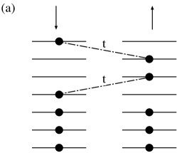
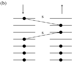
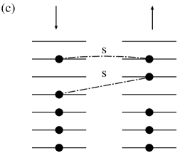
FIG. 1.: Distribution of off-diagonal interaction matrix elements (7) for a one-dimensional lattice model with nearest and next-nearest neighbor hopping and a Hubbard interaction (Details of the model can be found in reference [22]) and for different strength $W/V$ of the disordered potential $W/V=0$ (thin solid line), 1 (thick solid line), 2 (dashed line) and 3 (dotted-dashed line).

FIG. 2.: Representation of $\sigma_{z}=0$ many-body states with $\sigma=2$ (a) and 0 (b). These two states differ only by the nature of the two-particles bonds connecting pairs of fermions on partly filled orbitals which are either singlets or triplets (the nature of the bonds is indicated by the letter $s$ or $t$). As fermions on doubly occupied orbitals can only be singlet paired, they cannot provide for a nonzero spin. Together with SRS, this forbids the scattering from a triplet bond configuration onto a double occupancy, so that the rightmost state (c) can only be coupled to the $\sigma=0$ state (b).

FIG. 3.: Density of states for $n=2$, $m=12$ $\sigma=0$ (empty circles) and $\sigma=1$ (full circles) computed from 5000 realizations of ${\cal U}_{f}$. The full lines give the corresponding semicircle law (21). Tails develop due to the finiteness of the Hilbert space size ($N(0)=78$ and $N(1)=66$).

FIG. 4.: Average number $p$ of levels in the spin gap between the two yrasts for $n=2$, divided by the total number of levels $N(0)=m(m+1)/2$ in the $\sigma=0$ sector as a function of the number $m$ of one-particle orbitals. The dashed line shows the dependence $p/N\sim 1/N$ in agreement with a $m$-independent number of levels in the gap.

FIG. 5.: Average spin gap between the two lowest yrast levels (circles) and average splitting between the first excited $\sigma=0$ level and the $\sigma=1$ yrast level (triangles) of ${\cal U}_{f}$ for $n=2$ as a function of the number of one-particle orbitals $m$. The data show almost no $m$-dependence in agreement with (22).

FIG. 6.: Ground-state energy for the Hamiltonian (12) with $\lambda=0$ at $n=2$, $\sigma=0$, $m=12$ (circles) and $m=16$ (squares) as a function of the strength of off-diagonal fluctuations $U/\Delta$. The solid lines indicate the perturbative result $(\epsilon_{0,0}(U)-\epsilon_{0,0}(0))/\Delta=A(U/\Delta)^{2}$ with a numerical coefficient determined by (33) $A=-21.12$ and $-27.56$ respectively.

FIG. 7.: Ground-state energy for the Hamiltonian (12) with $n=2$, $\sigma=1$, $m=12$ (circles) and $m=16$ (squares) as a function of the strength of off-diagonal fluctuations $U/\Delta$ in absence of exchange interaction. The solid lines indicate the perturbative result $(\epsilon_{0,1}(U)-\epsilon_{0,1}(0))/\Delta=A(U/\Delta)^{2}$ with a numerical coefficient determined by (33)$A=-17.5$ and $-23.91$ respectively.

FIG. 8.: Spin gap between the two lowest yrast states for $n=2$ and $m=16$ as a function of the strength of off-diagonal fluctuations $U/\Delta$. The solid line gives the perturbative result from (35), giving $(\epsilon_{0,1}(U)-\epsilon_{0,0}(U))/\Delta=1+A(U/\Delta)^{2}$ with a numerical coefficient determined by (35), $A=3.66$.

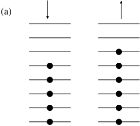
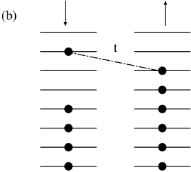
FIG. 9.: Energy of the $\sigma=0$ yrast state for $m=16$, $n=2$ (circles), 4 (squares), 6 (diamonds) and 8 (triangles), as a function of the strength of off-diagonal fluctuations $U/\Delta$. The solid lines give the perturbative results extracted from (46), giving $(\epsilon_{0,0}(U)-\epsilon_{0,0}(0))/\Delta=A(U/\Delta)^{2}$ with a numerical coefficient determined by (46)$A=-27.56$ $(n=2)$, -144.75 $(n=4)$, -281.09 $(n=6)$ and -373.57 $(n=8)$. Note that the breakdown of the perturbative expression coincides with the emergence of the large $U/\Delta$ linear regime.

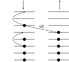
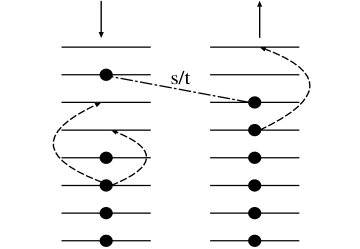
FIG. 10.: The two lowest yrast states $\sigma=1/2$ (a) and 3/2 (b) for odd number of fermions.

FIG. 11.: Left: Transitions that have a different transition amplitude for $\sigma=0$ and $\sigma=1$ and thereby give the dominant contribution to the spin gap between the two lowest yrast levels for even number of fermions. Right: Corresponding transitions for odd number of fermions giving different transition amplitudes for $\sigma=1/2$ and $\sigma=3/2$.

FIG. 12.: Rescaled spin gap between the two lowest yrast states for $m=16$ and $n=2$ (circles), 3 (squares), 4 (diamonds), 5 (triangles up), 6 (triangles left), 7 (triangles down) and 8 (triangles right). Symbols corresponding to odd (even) $n$ are filled (empty). The scaling parameter satisfies $\alpha=1$ (1.5) for even (odd) number of particles (see text). The scaling holds quite well already for a small number of particles $n\geq 4$ and the even-odd dependence of the gap confirms the theory presented in the text. Inset : spin gap before rescaling for the same cases as above. Lines corresponding to odd (even) $n$ are dashed (full) to stress the even-odd dependence of the gap. Note that for larger $n$, the gap starts to have a linear dependence above $U/\Delta\approx 0.1$ indicating the border between perturbative and asymptotic regimes.

FIG. 13.: Density of states for the Hamiltonian ${\cal U}_{f}$ with $n=6$ particles and $m=16$ orbitals, corresponding to the magnetization blocks $\sigma=-3$ (solid line), -2 (dotted line), -1 (dashed line) and 0 (dotted-dashed line). Inset: rescaled density of states showing the approximate scaling in $E/K^{1/2}U$.

FIG. 14.: Dependence of the finite-size spin gap in the number $n$ of particles in the regime of dominating fluctuations $U/\Delta\gg 1$ and $\lambda=0$. Points correspond to numerical results for $m=10$ (full circles), 12 (empty squares), 14 (full diamonds) and 16 (empty triangles). For the case $m=16$ and 1000 Hamiltonian realizations, the error bars indicate the r.m.s. of the gap distribution while the dashed and dotted-dashed lines show the numerically computed variances (Left-hand side of eq. (5.4)) for the full Hamiltonian and after setting to zero non-generic interaction matrix elements respectively.

FIG. 15.: Evolution of the energetic distance between the two lowest yrast for $n=5$ and $m=12$ as a function of the strength of interaction fluctuations $U/\Delta$. Shown are curves corresponding to an exchange $\lambda U/\Delta=0.$ (circles), 2 (squares), 4 (diamonds) and 6 (triangles). The error bar indicate the r.m.s of the distribution of $\Delta^{s}/\Delta$.

FIG. 16.: Probability for a magnetized ground-state as a function of the exchange $\lambda U/\Delta$ for 5000 realizations of Hamiltonian (12) with $n=6$, $m=12$. Three cases with equidistant (a), GOE (b) and random (c) one-body spectra are shown. Different curves correspond to different fluctuations of IME : $U/\Delta=0$ (solid line), 0.1,0.2,0.3…0.8, (symbols, from left to right).

FIG. 17.: Comparison of the ground-state magnetization probability for $n=6$ and $m=12$ at $U/\Delta=0$ (lines) and 0.5 (symbols) for equidistant (solid line and circles), Poissonian (dashed line and squares) and Wigner-Dyson (dotted-dashed line and diamonds) orbitals distribution.

FIG. 18.: Dependence of the average distance $\delta\lambda$ from the magnetization threshold $\lambda_{c}(U)$ for a Poissonian (squares) and Wigner-Dyson (diamonds) orbital distributions. $\lambda_{c}(U)$ is extracted from Fig. 24 as the value at which $P(\sigma>0)=0.01$ and $\lambda_{c}(U)+\delta\lambda$ corresponds to $P(\sigma>0)=0.5$. The linear fits do not extrapolate to zero since $P(\sigma>0)=0.5$ requires a finite $\delta\lambda$ at $U/\Delta=0$ (see Figs. 24).

FIG. 19.: Magnetization parameter $\lambda$ vs. disorder strength $W/V$, for a Hubbard interaction and a two-dimensional 10$\times$10 (full circles), 20$\times$20 (empty squares), 50$\times$50 (full diamonds) and 80$\times$80 (empty triangles) Anderson lattice. One clearly differentiates three regimes : (I) At small disorder, $\lambda$ increases due to a crossover from ballistic to diffusive behavior (see text). (II) At intermediate disorder, exchange and fluctuations compensate each other so that $\lambda$ is size-independent. (III) At large disorder one-body states are strongly localized over very few sites, which kills the off-diagonal fluctuations faster than the exchange and the latter dominates again.

FIG. 20.: Magnetization parameter $\lambda$ vs. disorder strength $W/V$, for a Hubbard interaction and a three-dimensional 6$\times$6$\times$6 (full circles), 8$\times$8$\times$8 (empty squares), 12$\times$12$\times$12 (full diamonds) and 15$\times$15$\times$15 (empty triangles) Anderson lattice. One clearly differentiates three regimes : (I) At small disorder, $\lambda$ increases due to a crossover from ballistic to diffusive behavior (see text). (II) At intermediate disorder, fluctuations seem to take over and $\lambda$ decreases with system size. (III) At large disorder one-body states are strongly localized over very few sites, which kills the off-diagonal fluctuations faster than the exchange and the latter dominates again.

FIG. 21.: Effect of the interaction range on the magnetization parameter $\lambda$ for a two-dimensional 15$\times$15 Anderson lattice and ratio ${\cal U}_{0}/{\cal U}_{1}=1$ (full circles), 4 (empty squares), 9 (full diamonds) and $\infty$ (Hubbard interaction - empty triangles). Increasing the interaction range leads to a stronger increase of the fluctuations than of the exchange, resulting in a lowering of $\lambda$.

FIG. 22.: Schematic of the conductance peaks in a 2D lateral quantum dot as a function of an in-plane magnetic field $g\mu_{B}B/\Delta$ for $m=14$, $\lambda U/\Delta=2$ (left) and 0.4 (right) and $U/\Delta=0.4$ corresponding to the addition of the $n=3,4,...9^{\rm th}$ electrons (from bottom to top). The dashed lines indicate slopes of $\pm g\mu_{B}/2$ and serve as a guide to the eye. At weak exchange (right), electrons are piled up on the orbitals according to the Pauli prescription, so that the spin is always minimized and the peaks move in parallel to the dashed lines. The sequence of magnetization difference between consecutive peaks $\delta\sigma_{z}(n)=(-1)^{n}/2$ results in peaks moving in opposite direction at low field. Larger slopes appear at larger exchange strength (left) and the successive addition of electrons of same spin results in conductance peaks evolving in parallel at low field. Note that due to the subtraction of the average charge-charge interaction, the model does not reproduce the charging energy so that the vertical distance between consecutive peaks is arbitrary.

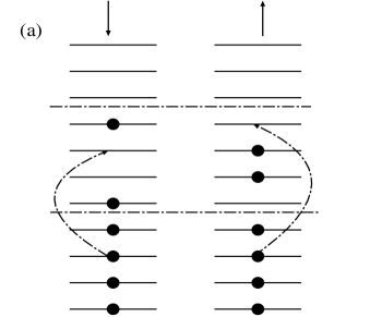
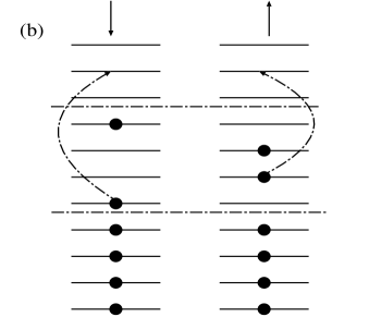
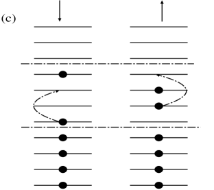
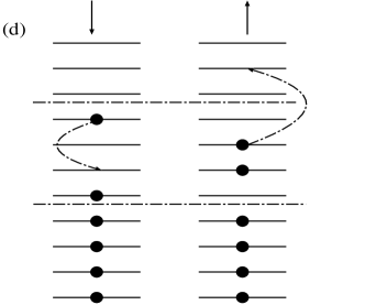
FIG. 23.: Representation of the $\sigma_{z}=0$ many-body yrast state with good total spin $\sigma$ at $U/\Delta=0$. The state consists of a filled fermi sea with $n/2-\sigma$ doubly occupied orbital and a layer of $2\sigma$ orbitals where particles are paired tripletwise.

FIG. 24.: Transitions that do not exist for the $\sigma\neq 0$ yrast state.

REFERENCES

- [1]
- [2] Ph. Jacquod and A.D. Stone, Phys. Rev. Lett. 84, 3938 (2000).
- [3] E.C. Stoner, Rep. Prog. Phys. 11, 43 (1947); see also S. Doniach and E. Sondheimer “Green’s Functions for Solid State Physicists”, Addison-Wesley (1974).
- [4] J. Hubbard, Proc. R. Soc. London A 276, 238 (1963); M.C. Gutzwiller, Phys. Rev. Lett. 10, 159 (1963).
- [5] For ferromagnetism in Hubbard-like models, see e.g. D. Vollhardt, N. Blümer, K. Held and M. Kollar, cond-mat/0012203 and J. Bünemann, F. Gebhard and W. Weber, Found. Phys. 30, 2011 (2000).
- [6] We will use the notations and for spin operators and and for the corresponding eigenvalues.
- [7] B.L. Altshuler and A.G. Aronov in “Electron-electron Interaction in Disordered Systems”, A.J. Efros and M. Pollak Eds, Elsevier (1985).
- [8] A.V. Andreev and A. Kamenev, Phys. Rev. Lett. 81, 3199 (1998).
- [9] P.W. Brouwer, Y. Oreg and B.I. Halperin, Phys. Rev. B 60, R13977 (1999).
- [10] H. U. Baranger, D. Ullmo and L. Glazman, Phys. Rev. B 61, R2425 (2000); D. Ullmo and H.U. Baranger, cond-mat/0103098.
- [11] U. Sivan et. al., Phys. Rev. Lett. 77, 1123 (1996); F. Simmel, T. Heinzel and D. A. Wharam, Europhys. Lett. 38, 123 (1997); S.R. Patel et. al., Phys. Rev. Lett. 80, 4522 (1998); F. Simmel et. al.,Phys. Rev. B 59, R 10441 (1999).
- [12] S. Lüscher, T. Heinzel, K. Ensslin, W. Wegscheider and M. Bichler, Phys. Rev. Lett. 86, 2114 (2001).
- [13] R. Berkovits, Phys. Rev. Lett. 81, 2128 (1998).
- [14] I.L. Kurland, I.L. Aleiner and B.L. Altshuler, Phys. Rev. B 62, 14886 (2000).
- [15] B.N. Narozhny, I.L. Aleiner and A.I. Larkin, Phys. Rev. B 62, 14898 (2000).
- [16] E. Eisenberg and R. Berkovits, Phys. Rev. B 60, 15261 (1999).
- [17] M. Stopa, Micro. Eng. 47, 119 (1999).
- [18] T.A. Brody, J. Flores, J.B. French, P.A. Mello, A. Pandey and S.S.M. Wong, Rev. Mod. Phys. 53, 385 (1981); K.K. Mon and J.B. French, Ann. Phys. 95, 90 (1975).
- [19] V.K.B. Kota, Phys. Rep. 347, 223 (2001).
- [20] Ph. Jacquod and A.D. Stone, Phys. Stat. Sol. 218, 113 (2000).
- [21] To avoid degeneracies in the many-body spectrum, we added in our numerics a small random part to the equidistant spectrum, , .
- [22] S. Daul and R.M. Noack, Phys. Rev. B 58, 2635 (1998).
- [23] P. Kopietz, Phys. Rev. Lett. 81, 2120 (1998).
- [24] Ya. M. Blanter and M. E. Raikh, Phys. Rev. B 63, 075304 (2001).
- [25] A.A. Abrikosov, L.P. Gor’kov and I.E. Dzialoshinskii, Methods of Quantum Field Theory in Statistical Physics, (Pergamon, New York, 1965).
- [26] L. Kaplan, T. Papenbrock and C.W. Johnson, Phys. Rev. C 63, 014307 (2001).
- [27] Note that this is a necessary but not sufficient condition. For example combining two , objects gives a nonzero component.
- [28] J. B. French and S.S.M. Wong, Phys. Lett. 33B, 447, (1970); 35B, 5 (1971); O. Bohigas and J. Flores, Phys. Lett. 34B, 261, (1971); 35B, 383 (1971).
- [29] L. Benet, T. Rupp and H.A. Weidenmüller, Phys. Rev. Lett. 87, 010601 (2001).
- [30] S. Åberg, Phys. Rev. Lett. 64, 3119 (1990); Ph. Jacquod and D. L. Shepelyansky, Phys. Rev. Lett. 79, 1837, (1997).
- [31] V. V. Flambaum, A.A. Gribakina, G.F. Gribakin and M.G. Kozlov, Phys. Rev. A 50, 267 (1994).
- [32] V. V. Flambaum, F. M. Izrailev and G. Casati, Phys. Rev. E 54, 2136 (1996).
- [33] M. Horoi, V. Zelevinsky and B.A. Brown, Phys. Rev. Lett. 74, 5194 (1995); V. Zelevinsky, B.A. Brown, N. Frazier and M. Horoi, Phys. Rep. 276, 85 (1996);
- [34] Y. Alhassid, Ph. Jacquod and A. Wobst, Phys. Rev. B 61, R13357 (2000); Y. Alhassid, Ph. Jacquod and A. Wobst, Physica E 9, 393 (2001); Y. Alhassid and A. Wobst, cond-mat/0003255.
- [35] Y. Alhassid, Rev. Mod. Phys. 72, 895 (2000).
- [36] B.L. Altshuler, Y. Gefen, A. Kamenev and L.S. Levitov, Phys. Rev. Lett. 78, 2803 (1997).
- [37] A.D. Mirlin and Y.V. Fyodorov, Phys. Rev. B 56, 13393 (1997);
- [38] X. Leyronas, J. Tworzydlo and C.W.J. Beenakker, Phys. Rev. Lett. 82, 4894 (1999).
- [39] C. Mejia-Monasterio, J. Richert, T. Rupp and H.A. Weidenmüller, Phys. Rev. Lett. 81, 5189 (1998).
- [40] P.H. Song, Phys. Rev. E 62, R7575 (2000).
- [41] B.L. Altshuler and B.I. Shklovskii, Zh. Eksp. Teor. Fiz. 91, 220 (1986) [Sov. Phys. JETP 64, 127 (1986)].
- [42] C.W. Johnson, G.F. Bertsch and D.J. Dean, Phys. Rev. Lett. 80, 2749 (1998); R. Bijker, A. Frank and S. Pittel, Phys. Rev. C 60, 021302 (1999); L. Kaplan and T. Papenbrock, Phys. Rev. Lett. 84, 4553 (2000); S. Drozdz and M. Wójcik, nucl-th/0007045; V.K.B. Kota and K. Kar, to be published.
- [43] For a special class of randomly interacting bosonic models a mapping onto random polynomials has been constructed which quantitatively reproduces the angular momentum distribution of the ground state : D. Kusnezov, Phys. Rev. Lett. 85, 3773 (2000).
- [44] M.L. Mehta, Random Matrices, Academic Press, New York (1991).
- [45] Note however that the ground-state distribution for the GOE has a typical width so that the distributions of the two yrasts strongly overlap; C.A. Tracy and H. Widom, Comm. Math. Phys. 87, 449 (1983).
- [46] A.D. Mirlin and Y.V. Fyodorov, J. Phys. A : Math. Gen. 24, 2273 (1991).
- [47] S.N. Evangelou, J. Stat. Phys. 69, 361 (1992).
- [48] Ya.M. Blanter, Phys. Rev. B 54, 12807 (1996).
- [49] Ya.M. Blanter and A.D. Mirlin, Phys. Rev. E 55, 6514 (1997).
- [50] Ph. Jacquod, cond-mat/0102345, in Proceedings of the 36th Rencontre de Moriond, “Electronic Correlations: from meso- to nano-physics”, G. Montambaux and T. Martin Eds.
- [51] This is already the case in the perturbative regime where this width is essentially determined by first order corrections. However the dependence in and is different.
- [52] We use indifferently for both even and odd even though in the latter case one should write .
- [53] These results should be considered as a limit as fluctuations are killed in a clean system.
- [54] V.N. Prigodin and B.L. Altshuler, Phys. Rev. Lett. 80, 1944 (1998).
- [55] Ya. M. Blanter, A.D. Mirlin, and B.A. Muzykantskii, Phys. Rev. Lett. 78, 2449 (1997).
- [56] This is not exactly true as the infinite-ranged interaction kills both fluctuations and exchange exactly. This result should be considered as a limit , .
- [57] D.S. Duncan, D. Goldhaber-Gordon, R.M. Westervelt, K.D. Maranowski and A.C. Gossard, Appl. Phys. Lett. 77, 2183 (2000); J. A. Folk, C. M. Marcus, R. Berkovits, I. L.Kurland, I. L.Aleiner and B. L. Altshuler, cond-mat/0010441.
- [58] Note that also in absence of fluctuations it is easier to magnetize an even number than an odd number of fermions as the doubling of the spin-gap at from to is only partially compensated by a 1.5-fold increase of the gain in exchange energy.
- [59] L.P. Rokhinson, L.J. Guo, S.Y. Chou and D.C. Tsui, Phys. Rev. B 63, 35321 (2001); L.P. Rokhinson, L.J. Guo, D.C. Tsui and S.Y. Chou, cond-mat/0102107.
- [60] There is however a non negligible coupling between the transverse component of the electronic wavefunction and the magnetic field : F. Stern, Phys. Rev. Lett. 21, 1687 (1968). This coupling causes a large, common energy shift of all the conductance peaks and experimentally, one commonly subtract it by considering the spacings between neighboring peaks [57]. We are indebted to D. Goldhaber-Gordon for pointing this out to us.
- [61] D. Weinmann, W. Häusler and B. Kramer, Phys. Rev. Lett. 74, 984 (1995).
- [62] A.M. Finkelstein, Zh. Eksp. Teor. Fiz. 84, 168 (1983) [Sov. Phys. JETP 57, 97 (1983)]; Z. Phys. B 56, 189 (1984); see also C. Chamon and E. Mucciolo, Phys. Rev. Lett. 85, 5607 (2000).
- [63] C. Castellani, C. Di Castro, P.A. Lee, M. Ma, S. Sorella and E. Tabet, Phys. Rev. B 30, 1596 (1984).