Thermodynamic Properties of the Dimerised and Frustrated $S=1/2$ Chain

Abstract

By high temperature series expansion, exact diagonalisation and temperature density-matrix renormalisation the magnetic susceptibility $\chi(T)$ and the specific heat $C(T)$ of dimerised and frustrated $S=1/2$ chains are computed. All three methods yield reliable results, in particular for not too small temperatures or not too small gaps. The series expansion results are provided in the form of polynomials allowing very fast and convenient fits in data analysis using algebraic programmes. We discuss the difficulty to extract more than two coupling constants from the temperature dependence of $\chi(T)$.

Dedicated to Professor E. Müller-Hartmann on occasion of his 60^th birthday.

I Introduction

Quantum spin systems are amongst the most interesting and challenging problems of many-body theory in solid state physics. Due to their intrinsic many-body quantum character it is not possible to compute even simple quantities like magnetic susceptibilities or specific heats in a straightforward fashion. But there are by now a number of powerful approaches like exact diagonalisaton, quantum Monte Carlo, temperature density-matrix renormalisation or high temperature series expansion which yield the desired quantities.

The first aim of our present paper is to provide high temperature series data which in combination with some $T=0$ information can serve as an input for quick data analysis. High order series expansions constitute an efficient, frequently used technique gelfa00 . Exact diagonalisation and temperature density-matrix renormalisation will serve as benchmarks to assess the reliability of the method proposed. Similar analyses are carried out in Refs. johns00a, ; johns00b, for unfrustrated dimerised spin chains and ordinary spin ladders.

The second aim of our work is to demonstrate that it is essentially impossible to deduce from one quantity like the magnetic susceptibility $\chi(T)$ at not too small temperatures alone more than two of the three magnetic couplings of dimerised and frustrated spin chains. This should caution anybody who is analysing such data in great detail. To illustrate the type of problem one can run in we refer the reader to the analysis of (VO)₂P₂O₇ which was analysed in the very beginning as dimerised chain johns87 . Then it was thought to be a two-leg spin-ladder with $J_{||}\approx J_{\perp}$ eccle94 . But lately unambiguous evidence from inelastic neutron scattering was found garre97a that it is a set of weakly coupled dimerised chains proko98 ; uhrig98c . The magnetic susceptibility $\chi(T)$ is compatible with both scenarios barne94 .

In this article we focus on gapped one-dimensional spin systems. These form a rather large class comprising dimerised spin chains, strongly frustrated spin chains but also spin ladders, cf. Fig. 1. A representative for a moderately dimerised spin chain is (VO)₂P₂O₇ garre97a ; proko98 ; uhrig98c ; a strongly dimerised spin chain realised in Cu₂(1,4-C₅H₁₂N₂)₂Cl₄ chabo97a ; chabo97b ; hamma98 ; elstn98 ; an example for a significantly frustrated spin chain is the spin-Peierls substance CuGeO₃ (see e.g. Ref. knett01a, and the discussion therein) which is undimerised in its high temperature phase ($T>T_{C}\approx 14$K) but weakly dimerised in its low temperature phase. An important spin ladder compound is SrCu₂O₃ azuma94 .

All these substances are interesting because they constitute disordered antiferromagnets with low coordination number. This means that their ground state is not given by a Néel-type state (i.e. with finite sublattice magnetisation) but by a Resonating-Valence Bond (RVB) state made of superposed singlet-product states liang88 . If the systems are indeed gapped the average range of the singlet pairs present in the ground state is finite. In other words, the correlation length is finite. Generally, an RVB state is favoured over a Néel state by low coordination numbers, by low values of the spin and by frustration (which simply weakens the classical ordered Néel-state).

If it is possible to dope the insulating magnetic systems unusual electronic properties emerge due to the strong interplay between charge and spin degrees of freedom. Some spin ladders like Sr_0.4Ca_13.6Cu₂₄O_41.84 become even superconducting under pressure uehar96 . Of course, the appearance of a true phase transition at finite temperatures requires a higher dimensionality than one mermi66 ; hohen67 ; nagat98 . But the driving mechanisms can be present already in the low-dimensional systems. So, a deeper understanding of unusual electronic behaviour in doped antiferromagnets requires a thorough understanding of the magnetic subsystem. It is in this context that we perform the present investigation which is designed to determine the relevant magnetic couplings easily and reliably.

Starting point of our theoretical study is the Hamilton

$$H=\sum_{i=1}^{N}\left(J\left[\left(1+(-1)^{i}\delta\right)S_{i}S_{i+1}+\alpha S_{i}S_{i+2}\right]\right)$$ (1)

with dimerised nearest and and uniform next-nearest neighbour interaction. The dimerisation is parameterised by $\delta$. The ratio of nearest and next-nearest neighbor interaction is given by $\alpha$. The dimerisation can arise from chemically different bonds as is the case in (VO)₂P₂O₇. Alternatively, it may be induced by a static lattice distortion via spin-phonon coupling as in CuGeO₃. The Hamiltionian can also be viewed as a spin ladder with an extra diagonal coupling $(1-\delta)J$ (see Fig. 1). In the limit $\delta=1$ it is equivalent to a regular ladder model. In the limit $\delta=1$, $\alpha=0$ a system of isolated dimers is obtained.

Figure 1: Dimerised and frustrated $S=1/2$ spin chain. For $\delta=1$ a two-leg ladder is obtained.

The ground state properties of the model (1) are investigated recently in numerous papers, see e.g. chitr95 ; uhrig96b ; uhrig96be ; white96 ; brehm96 ; yokoy97 ; brehm98 ; knett00a .

In the next section II we discuss briefly aspects of the methods we employ. The subsequent section III is devoted to the results for the magnetic susceptibility $\chi(T)$. In particular, we will discuss to which extent several couplings can be deduced reliably from $\chi(T)$ data alone. Section IV contains the results for the specific heat. We discuss how much can be learnt from $C(T)$ data. The Summary V concludes this article.

II Methods

The present work is concerned with the finite temperature properties of the magnetic susceptibility $\chi(T)$ and the magnetic specific heat $C(T)$. The analytic method we use is high temperature series expansion (HTSE). Its results are obtained as polynomials in the coupling parameters with fractions of integers as coefficients so that no accuracy is lost. Details of the calculation are found in Ref. buhle00, . Furthermore, the data is provided in electronic form so that they can be put to use quickly. In order to maximise the range of applicability some extrapolation schemes are necessary which are described below in detail.

In addition, we use numerical methods to cross-check the validity of the analytic results and to supplement them where necessary. A statistical method is quantum Monte Carlo (QMC) evert93 . In its present form, however, it suffers from the sign problem for frustrated systems so that we use it only in the unfrustrated cases. Mostly we employ the method of exact diagonalisation (ED) for smaller finite clusters bonne66 ; fabri98a . It is based on the determination of all eigen-values so that the partition sum can be computed directly. Thereby any thermodynamic quantity is accessible. For not too low temperatures the results describe reliably the thermodynamic limit. The third technique that we use is temperature density-matrix renormalisation (T-DMRG)klump99a ; johns00b . By this numerical method very low temperatures can be reached reliably.

We deal with the static magnetic susceptibility

$$\chi(\beta;\delta,\alpha)=\frac{\beta}{N}\frac{\mathrm{tr}M^{2}e^{-\beta H}}{\mathrm{tr}e^{-\beta H}}=\frac{\beta}{N}\langle M^{2}\rangle$$ (2)

and the specific heat

$$C(\beta;\delta,\alpha)=\frac{1}{N}\frac{\partial}{\partial T}\left(\frac{-\frac{\partial}{\partial\beta}\mathrm{tr}e^{-\beta H}}{\mathrm{tr}e^{-\beta H}}\right)$$ (3)

In the Appendices the series coefficients are given. For the dimerised and frustrated chain the coefficients for both quantities $\chi(T)$ and $C(T)$ are provided up to order 10 in the inverse temperature $\beta$. For the unfrustrated dimerised chain they are given up to order 18. The bare truncated series, however, are not sufficient to describe the quantities under study at low values of $T$. To enhance the region of validity of the high temperature series expansion Dlog-Padé representations domb89 are used. We show in the following that the complete susceptibility of gapped spin chains can be obtained if some low temperature information is incorporated in a simple way. This is explained subsequently in detail.

A Dlog-Padé approximant of the expansion of the magnetic susceptibility $\chi(\beta)$ is given by

$$\chi(\beta)=\frac{1}{4T}exp\left(\int\limits_{0}^{\beta}P^{k}_{l}(\beta^{\prime})d\!\beta^{\prime}\right)\ ,$$ (4)

where $P^{k}_{l}(\beta^{\prime})$ is the rational Dlog-Padé approximant with a polynomial of degree $k$ in the numerator and a polynomial of degree $l$ in the denominator of

$$f=\partial_{\beta^{\prime}}\ln(4T\chi(\beta^{\prime}))=\frac{\partial_{\beta^{\prime}}4T\chi}{4T\chi}\ .$$ (5)

Possible orders $[k,l]$ of $P_{l}^{k}(\beta)$ have to fulfill $k+l=n-1$ where $n$ is the order of the truncated series available. This can be seen by comparing the number of series coefficients obtained and the number of independent (one less than the total number) coefficients in the two polynomials of $P_{l}^{k}(\beta)$. Due to the derivative on the right side of (5) one coefficient of the series expansion is lost.

Additionally, we incorporate $T=0$ information to supplement the high temperature expansion. In the case of ungapped spin chains buhle00 we used knowledge of the full dispersion for this purpose. Though successful this approach is cumbersome in general. Therefore, we now simplify the procedure to incorporate $T=0$ information considerably. It is described for the case of gapped spin chains.

At zero temperature the susceptibility of a gapped system vanishes and at finite but small temperature the deviation is exponentially small due to the spin gap $\Delta$

$$\chi(T)\approx e^{-\frac{\Delta}{T}}\ \text{ for T}\ll\Delta\ .$$ (6)

Furthermore, the leading power in $T$ can be determined on the basis of the dimensionality of the problem and of the behaviour of the dispersion close to its minima. For one-dimensional systems with quadratic minima , which is generic for gapped systems, one obtains troye94

$$\chi(T)\approx\frac{1}{\sqrt{T}}e^{-\frac{\Delta}{T}}\ \text{ for T}\ll\Delta\ .$$ (7)

This equation provides information for two additional coefficients of the Dlog-Padé approximant. Let us extend the series expansion of $\chi$ by two terms $a\cdot\beta^{n+1}+b\cdot\beta^{n+2}$ yielding $\chi_{\rm e}$. Then the degree of the approximant $P_{l}^{k}(\beta)$ can be incremented by two fulfilling $k+l=n+1$. The two additional conditions deriving from (7) follow from

$$P_{l}^{k}(\beta)=-\Delta-1/(2\beta)+\mathcal{O}(\beta^{-2})$$ (8)

in the limit $\beta\to\infty$. This condition requires that $P_{l}^{k}(\beta)$ is finite for $\beta\to\infty$ imposing the severe constraint $l=k$ on the possible degrees of the Dlog-Padé approximant. To circumvent this constraint we substitute

$$u=\beta/(1+\beta)\Leftrightarrow\beta=u/(1-u)$$ (9)

thereby mapping the complete $\beta$-interval $[0,\infty]$ to the $u$-interval $[0,1]$. This mapping is justified by the continuity of $P_{l}^{k}(\beta)$ in the limit $\beta\rightarrow\infty$.

The asymptotic behaviour (8) transforms under the mapping (9) to

$$P^{k}_{l}(u)\Big{|}_{u=1} = -\Delta$$ (10a)

$$\partial_{u}P^{k}_{l}(u)\Big{|}_{u=1} = 1/2\ ,$$ (10b)

where we use $P^{k}_{l}$ now for the rational function in $u$. We will henceforth consider only approximants in $u$ so that no confusion should arise.

The Dlog-Padé approximant $P_{l}^{k}(u)$ is chosen such that it approximates $\partial_{u}4T\chi_{\rm e}/4T\chi_{\rm e}$ where $\beta$ is expressed according to (9) as function of $u$. In this way, reliable interpolations between the low temperature behaviour and the high temperature series expansion can be obtained for arbitrary orders $k$ and $l$ complying with $k+l=n+1$.

To assess the range of validity of the Dlog-Padé approximant various orders of $P^{k}_{l}$ are investigated. Examination of the positions $\beta_{i}$ of the poles of $P^{k}_{l}$ and especially of the largest modulus of them leads to a reliable estimate of the radius of convergence $\beta_{\rm r}$ of the series in $\beta$ (Cauchy’s theorem). We find roughly $\beta_{\rm r}\approx 2/J$ as for the ungapped spin chains buhle00 . This means that the truncated series will always diverge around $T\approx 0.5J$ even for arbitrary high order in $\beta$. Thus the polynomial representation is not sufficient to describe the maximum of $\chi(T)$ quantitatively.

III Magnetic Susceptibility $\chi(T)$

III.1 Applicability of the High Temperature Series Expansion

In Fig. 2 various representations of the susceptibility are shown and compared. For fixed order $l$ of $P_{l}^{k}$ the Dlog-Padé representation of $\chi$ moves for $l=2$ upwards, for $l=4$ downwards and for $l=5$ in both directions (for $l=3$ no evaluation is possible due to defective approximants in all orders). All representations converge for increasing order.

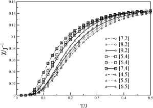
Figure 2: Susceptibility for $\delta=0.1$ and $\alpha=0.24$ for the dimerised, frustrated spin-1/2 chain. Various orders of the Dlog-Padé approximant are shown.

Figure 3: Susceptibility of the dimerised chain for various values of $\delta$. The Dlog-Padé approximants are of order $[15,4]$

The $[5,4]$ and $[4,5]$ approximants cannot be discerned. But this is not a general feature. Other reflected approximants of the type $[k,l]$ and $[l,k]$ yield substantially differing results. In order to present our results in a systematic and unbiased way we choose the $P^{m}_{4}$ representation for all curves shown below (if not denoted otherwise). Deduced from Fig. 2 we expect quantitatively reliable results down to $T/J\approx 0.25$ for the dimerised, frustrated chain. This conclusion is based on considering the highest orders and on looking for the range of $T/J$ where they are consistent.

In the purely dimerised case, see Fig. 3, almost the whole temperature regime is excellently described. This is due to the high orders reached ($\mathcal{O}(\beta^{18})$). In Fig. 3, the HTSE results are depicted in comparison to results from numerical methods (ED, QMC) and the exact result of the uniform chain klump93b . In particular, the agreement between the HTSE result and the exact one for the uniform chain is impressive. We think that this is the optimum which can be obtained by high temperature expansion since it is certainly not possible to assess the logarithmic low temperature corrections coming from the high temperature end. Technically, we used for the uniform chain instead of (10) the obvious relations

$$P^{k}_{l}(u)\Big{|}_{u=1} = 0$$ (11a)

$$\partial_{u}P^{k}_{l}(u)\Big{|}_{u=1} = 1\ .$$ (11b)

The second relation (11b) reflects the fact that $\chi(0)$ is finite.

In Fig. 4

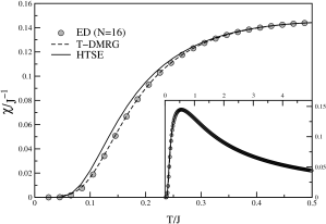
Figure 4: Comparison of high temperature series expansion, exact diagonalisation and temperature density-matrix renormalisation data for $\alpha=0.24$ and $\delta=0.1$.

the $[7,4]$ HTSE representation chosen is compared to exact diagonalisation and temperature density-matrix renormalisation data klump99a . The results are in very good accordance with each other. Only in the regime $T/J<0.2$ there is a slight difference between the HTSE representation and the numerical results.

In Fig. 5 the susceptibilities for various sets of parameters are shown. The behaviour of the maximum of the susceptibility depends upon the parameters under study. For fixed next-nearest neighbour interaction $\alpha$ the position of the maximum moves to higher values of $T/J$ for increasing $\delta$ while the maximum value decreases. These effects are induced by the increasing gap.

Fixing $\delta$, the position of the maximum moves to the left for increasing $\alpha$. This can be understood from the reduction of the dispersion on increasing frustration. The mobility of the excitations is more and more restricted uhrig96b ; uhrig96be ; knett00a . The maximum value of $\chi(T)$ remains almost constant. This can be seen as the result of an compensation of two contrary effects. On the one hand, the susceptibility would rise due to the shift of the maximum position to lower temperatures where the global $1/T$ factor (cf. (2)) enhances its value. But on the other hand, the frustration provides an additional antiferromagnetic coupling in the system which works against an alignment of the spins. For instance, the antiferromagnetic next-nearest neighbour coupling induces a strong repulsion between aligned adjacent triplets on the dimers uhrig96b ; uhrig96be ; knett00a .

Figure 5: Susceptibility for various values of $\delta$ and $\alpha$. Representation by the $[7,4]$ approximant except for the solid line in the uppermost panel where the $[7,4]$ approximant is defective and the $[8,3]$ approximant is used.

III.2 Information Content of $\chi(T)$

In this section we address the question to which extent the parameters of the model Eq. 1 can be extracted from measurements of the susceptibility. In other words, we adopt the experimentalist’s point of view who wants to determine the coupling parameters from experimental data. Obviously, the main feature in the susceptibility curve is the maximum. So it is natural to use in the first place the maximum value $\chi_{\rm max}$ and its position $T=T_{\rm max}$. We consider the product $\chi_{\rm max}T_{\rm max}$ since it is experimentally easily accessible and does not depend on the exchange coupling $J$.

The data shown in Fig. 6 are obtained by exact diagonalisation of the full Hamitonian of a 16 site system. For $\alpha<0.75$ the data are exact to many digits for a system of this size. For $\alpha>0.75$ and $\delta=0$ finite-size effects of several percent occur.

Note that for $\delta=0$ the quantity $\chi_{\rm max}T_{\rm max}$ reaches its minimum at $\alpha\approx 0.5$ and then starts to increase again. This is due to the fact, that on growing $\alpha$ the system approaches two independent chains of half the size of the original chain with $\alpha=0$.

Figure 6: $\chi_{\rm max}T_{\rm max}$ versus $\delta$ for $\alpha=0.0,0.12,0.24,0.36,0.50,0.75,1.0,2.0$ and $4.0$ (in descending order at the right side of the graph, i.e. $\delta=1.0$). The symbols are obtained by analysing the HTSE showing excellent agreement with the numerical data. For illustration, the dashed line refers to the experimental value of (VO)₂P₂O₇.

Fig. 6 can be used easily: given the experimental input for $\chi_{\rm max}T_{\rm max}$ one can read off the value for $\delta$ for a chosen $\alpha$.

To complete the analysis we plot in Fig. 7 the variable $J/T_{\rm max}$ as a function of $\delta$ for various values of $\alpha$. So, once the value of $\delta$ (for given $\alpha$) is determined from Fig. 6, Fig. 7 helps to determine the exchange coupling $J$ by reading off $J/T_{\rm max}$ and multiplying by $T_{\rm max}$.

Figure 7: $\frac{J}{T_{max}}$ versus $\delta$ for $\alpha=0.5,0.36,0.75,0.24,1.0,0.12,0.0,2.0$ and $4.0$ (in descending order at the left side i.e. $\delta=0.0$).

We want to point out here that it is almost impossible to determine the values of $J$, $\alpha$ and $\delta$ from the temperature dependence of the susceptibility alone (cf. also low00, ). This phenomenon is well known from the investigations of (VO)₂P₂O₇. In the case of this substance the susceptibility of the isotropic ladder i.e. a ladder with $J_{||}=J_{\perp}$ and the susceptibility of a dimerised spin chain with $\delta=0.2$ fit both the experimental data equally well. For illustration the possible results for (VO)₂P₂O₇, where $\chi_{\rm max}=2.07\ 10^{-3}$ emu/mol V and $T_{\rm max}=74K$ correspond to the horizontal dashed line at 0.15 emu K/mol V in Fig. 6.

Figure 8: Re-scaled susceptibilities for $\chi_{\rm max}T_{\rm max}$= 0.17, 0.16, 0.15, 0.14, 0.13 emu K/mol for the $\alpha$ and $\delta$ values shown in Fig.  9 ($g$-factor set to 2).

The difficulty to distinguish different sets of ($J,\delta,\alpha$) yielding the same value of $\chi_{\rm max}T_{\rm max}$ is visualised strikingly in Fig. 8. The re-scaled susceptibilities belonging to various values of $\chi_{\rm max}T_{\rm max}$ are depicted. In the temperature region around the maxima and for larger temperatures the differences within each set are minute. Thereby we conclude that it is impossible to determine all three coupling parameters from $\chi(T)$ at moderate and at large values of temperature alone. In Fig. 9 the values of $\alpha$ and $\delta$ are shown which belong to the various sets displayed in Fig. 8.

Figure 9: Lines of constant height $\chi_{\rm max}T_{\rm max}$= 0.17,0.16,0.15,0.14,0.13 emu K/mole in the $\alpha$-$\delta$ plane.

Next we use the high temperature expansion results (see Appendix A2) to understand such a scaling behaviour in the lowest orders of $\beta$. It is obvious that the zeroth order $4T\chi\approx 1$ does not allow the determination of any parameters. The first order of the susceptibility of a model with given frustration $\alpha$ and exchange coupling $J$ is identical to the first order of another model with frustration $\alpha_{1}$ and coupling $J_{1}$ if

$$J_{1}(1+\alpha_{1})=J(1+\alpha)$$ (12)

holds. In other words, if one had only first order results for the susceptibility it would be impossible to determine $J$ and $\alpha$ independently.

The second order of the HTSE depends on $\delta$. But again one can choose a particular value $\delta_{1}$ such that the sets $(J,\alpha,\delta)$ and $(J_{1},\alpha_{1},\delta_{1})$ lead to identical zeroth, first and second order terms in $\beta$. This choice is

$$\delta_{1}^{2}=2\alpha_{1}-(2\alpha-\delta^{2})\left(\frac{1+\alpha_{1}}{1+\alpha}\right)^{2}\ .$$ (13)

If the susceptibility is determined mainly by the first three orders the relations (12,13) provide the recipe to re-scale the susceptibility such that different parameter sets yield similar temperature dependences. Indeed, if one focuses on the high temperature range this is true. The precise position and value of the maxima, however, cannot be deduced from the first three orders alone. This implies that Eq. 13 provides only rough estimates for the curves displayed in Fig. 9.

To be cautious, we like to stress that we are not claiming that it is impossible to determine all three coupling $J,\alpha,\delta$ if sufficient low temperature data is available to obtain the value of the gap. The gap $\Delta$ depends in a different way on the couplings than $\chi(T)$ does knett00a . Very often, however, the dependence at low values of the temperature is either not accessible or it no longer corresponds to a pure 1D system. In particular, interchain couplings $J_{\perp}$ lead to significantly altered gaps (for examples see Refs. knett01a, ; uhrig01a, ) although the behaviour at higher temperatures $T>J_{\perp}$ is still well described by a 1D model.

IV Specific Heat $C(T)$

It is a straightforward idea to extract further information about the magnetic properties of certain materials by considering also the specific heat $C$. Only in very rare cases, however, the magnetic part of $C$ can be extracted in a reliable way from the measured data because the phononic contributions dominate $C$ whenever the energy scale of the lattice vibrations is of the order of the magnetic coupling $J$.

At low temperatures where the phononic contributions vanish following the usual $T^{3}$ law a reliable extraction of $C$ is possible. For high temperatures such a procedure will fail in general as can be seen, for instance, in a simple model of Einstein (dispersionless) phonons coupled to Heisenberg chains kuhne99b . So the full temperature dependence of the magnetic part of $C$ can be measured only in substances with a small exchange coupling $J$ as it occurs, for instance, in organic magnetic materials, see e.g. Ref. rapp95, .

Furthermore, it is in order to mention that there are indirect techniques to obtain the magnetic part of $C(T)$ where the energy fluctuations are linked to dissipation. The latter is measured by the intensity of elastic scattering in spectroscopic investigations, see e.g. kuroe97 ; grove00 . The indirect approaches, however, may provide information on $T_{\rm max}$ of $C(T)$ but not on $C_{\rm max}$ itself since overall factors are not known. (In this section $T_{\rm max}$ refers always to $C(T)$. The position of the maximum of $\chi(T)$ is denoted $T_{\rm max}^{\chi}$.)

In the Appendices A and B the coefficients for the specific heat are provided. In order to compute $C(T)$ additional information on the low temperature behaviour is included as was done for $\chi(T)$. At zero temperature the magnetic specific heat of a gapped system vanishes and at finite but small temperatures the deviation is exponentially small. For one-dimensional systems one has troye94

$$C(T)\propto T^{\frac{3}{2}}e^{-\frac{\Delta}{T}}\ .$$ (14)

This asymptotic behaviour leads to a Dlog-Padé representation of $C$ equivalent to the one of the susceptibility (see Eqs. 4 to 10). The function approximated by $P_{l}^{k}$ reads

$$g=\partial_{\beta}\ln\left(\left[\frac{3}{16}\left(1+\delta^{2}+\alpha^{2}\right)\beta^{2}\right]^{-1}C(\beta)\right)$$ (15)

where the additional factor ensures that the argument of the logarithm tends to unity for $\beta\to 0$. As for the susceptibility two additional terms are taken into account which are determined such that the correct asymptotics in $u=\beta/(1+\beta)$ is guaranteed

$$P_{l}^{k}(u)\big{|}_{u=1} = -\Delta$$ (16)

$$\partial_{u}P_{l}^{k}(u)\big{|}_{u=1} = 7/2\ .$$ (17)

Figure 10: Specific heat $C$ for various values of $\delta$ and $\alpha$. The Dlog-Padé approximants used are of degree $[5,4]$ for the frustrated and dimerised chains and $[13,4]$ for the chains without frustration.

In Fig. 10 the specific heat for various sets of parameters $\alpha$ and $\delta$ is compared to numerical ED and T-DMRG results. For large enough dimerisation $\delta$, the ED and HTSE results agrees perfectly. For $\delta=0.1$ and $\alpha=0.24$ the HTSE describes the position of the maximum of the specific heat very well, but the absolute value deviates slightly from the ED and the T-DMRG results. This problem arises since the maximum in the specific heat occurs at fairly low values of $T/J\approx 0.3$. In the purely dimerised case where we have reached 18^th order in $\beta$, the HTSE describes the maximum perfectly. Only in the regime $T/J<0.25$ there is a slight difference to the ED and to the T-DMRG results. The same is true for the uniform chain (see inset of Fig. 10) where some deviations from the exact solution occur well below $T_{\rm max}$. We attribute these deviations below the maximum position $T_{\rm max}$ to logarithmic corrections which cannot be assessed by the high temperature series expansion.

Figure 11: Re-scaled specific heat $C$ for various values of $\delta$ and $\alpha$ all yielding the same value $\chi_{\rm max}T^{\chi}_{\rm max}=0.15$ emu K/mol.

Fig. 11 displays $C(T)$ for the points in Fig. 9 belonging to $\chi_{\rm max}T^{\chi}_{\rm max}=0.15$ emu K/mol. Therefore, the temperature dependence is given in units of the maximum temperature $T^{\chi}_{\rm max}$ of the susceptibility. Clearly, the curves differ from each other. Hence the knowledge of $C(T)$, in addition to the knowledge of $\chi(T)$, renders a complete determination of all three couplings possible. This is our main point in the present section. In other words, the knowledge of $\chi(T)$ allows to fix $\delta$ and $J$ for given $\alpha$. But $\alpha$ cannot be determined easily since there are sets of parameters leading to very similar $\chi(T)$ curves, see Fig. 8. The corresponding $C(T)$ curves, however, differ significantly as illustrated in Fig. 11 and thus provide a proper distinction of different parameter sets.

To complete our analysis for the specific heat we provide for $C(T)$ in the Figs. 12 and 13 the analoga of Figs. 6 and 7 for $\chi(T)$. Fig. 12 displays the dimensionless (if $k_{\rm B}$ is set to unity) specific heat which is independent of the value of the exchange coupling $J$. For given dimerisation $\delta$ the frustration parameter $\alpha$ can be read off. Once $\alpha$ is known the curves in Fig. 13 allow to determine the energy scale.

Figure 12: Maximum value $C_{\rm max}$ of the specific heat as function of the frustration $\alpha$ for various values of the dimerisation $\delta$. For $\delta=0$ no data is shown beyond $\alpha=0.5$ since the exact diagonalisation results are not reliable there.

Figure 13: Position $T_{\rm max}$ of the maximum of $C(T)$ as function of the frustration $\alpha$ for various values of the dimerisation $\delta$. For $\delta=0$ no data is shown beyond $\alpha=0.5$ since the exact diagonalisation results are not reliable there.

Let us briefly describe the principal behaviour of $C(T)$ as a function of $\delta$ and $\alpha$. Some of the features of the curves can be understood by simple arguments. In Fig. 12 all curves converge to the dotted line for increasing values of $\alpha$. The value of the dotted line is $C_{\rm max}$ of a uniform chain without dimerisation and frustration. This is implied by the simple fact that the system approaches the limit of two independent chains for $\alpha\to\infty$. Then the couplings $J(1+\delta)$ and $J(1-\delta)$ between the two legs (cf. Fig. 1) become less and less important

$$\lim_{\alpha\to\infty}C_{\rm max}(\alpha,\delta)=C_{\rm max}(\alpha=0,\delta=0)\ .$$ (18)

For fixed value of the dimerisation $\delta$ the position $T_{\rm max}$ of the maximum of $C$ is shifted to lower values on increasing $\alpha$. This can be understood by the suppression of the dispersion of the elementary excitations due to the frustration uhrig96b ; uhrig96be ; knett00a . Thereby the overall energy scale on which excitations exist is reduced. The same was observed for the susceptibility as shown in the preceding section. A minimum is reached for a certain value of $\alpha\approx 0.5$ because $T_{\rm max}$ has to rise again since the system approaches the limit of two independent chains. Quantitatively, the large $\alpha$ limit fulfills

$$\lim_{\alpha\to\infty}\frac{T_{\rm max}(\alpha,\delta)}{J\alpha}=\frac{T_{\rm max}(\alpha=0,\delta)}{J}\ .$$ (19)

independent of $\delta$.

It should be noted that for large $\delta$ (cf. Fig. 13) the value of $C_{\rm max}$ does not substantially change which makes it difficult to discriminate the curves experimentally. The data shown are obtained for a $N=16$ cluster. A finite size analysis shows that the finite cluster results coincide with the infinite chain result except for points with $\delta=0$ and $\alpha>0.5$.

V Summary

The aim of the present article was two-fold. In the first place, we provided results and tools to facilitate and to expedite the analysis of experimental data in terms of a one-dimensional $S=1/2$ model, namely dimerised and frustrated spin chains. This model can also be seen as zig-zag chain and comprises in particular the usual spin ladder. Secondly, we demonstrated to which extent it is possible to determine the model parameters quantitatively from the temperature dependences of the magnetic susceptibility $\chi$ and of the specific heat $C$.

We showed in detail how analytic high temperature series in high orders can be used to obtain reliable approximants, namely Dlog-Pad e approximants. The key point is to use additional well-known information on the $T=0$ and on the low-temperature behaviour to stabilise the approximants in the low-temperature region. We use the size of the gap, the form (linear or quadratic) of the dispersion in the vicinity of its minimum and the dimensionality of the system as additional input. Thereby we achieve very good results in a straightforward fashion. The validity of the results is comparable to the one achieved by another extrapolation procedure introduced previously buhle00 . The approach used in the present work is simpler since it requires less additional input. In Ref. buhle00, knowledge of the whole dispersion was used.

With the help of a computer algebra programme the approximants can be computed very quickly and easily. Thereby efficient data analysis becomes possible.

The extrapolated series expansion results were gauged carefully by comparing them to numerical data. The methods employed are exact diagonalisation, quantum Monte Carlo and temperature density-matrix renormalisation.

To ease data analysis further we included in the present work results for many sets of parameters. Figs. 6, 7, 12 and 13 make it possible to read off the coupling parameters $J,\alpha$ and $\delta$ if as little as the maximum values of the magnetic susceptibility, of the specific heat and the corresponding positions $T_{\rm max}^{\chi}$ and $T_{\rm max}^{C}$ are known.

It turned out that the knowledge of $\chi(T)$ at moderate and high temperatures alone is not sufficient to determine the three model parameters. Any additional knowledge, for instance on $C(T)$ or on the singlet-triplet gap $\Delta$, solves the problem. But such additional information is difficult to obtain. The specific heat is mostly dominated by the phonon contribution making it difficult to be extracted. The gap $\Delta$ is in principle well defined. Frequently, however, the real systems lose their one-dimensionality at low energies, for instance due to small interchain couplings. Then the gap is influenced decisively by these additional residual couplings although the behaviour at moderate and higher temperatures is perfectly described by a one-dimensional model. In the analysis of experimental data it is certainly helpful to consider these facts.

Appendix A Dimerised and frustrated chain

A.1 Specific heat

Table 1: Series coefficients $a_{n,k,l}$ for the high temperature expansion of the magnetic specific heat of the dimerised, frustrated chain $C=\sum_{n,k,l}a_{n,k,l}\alpha^{k}\delta^{l}(\beta J)^{n}$. Only nonzero coefficients are presented.

(n,k,l)	$a_{n,k,l}$	(n,k,l)	$a_{n,k,l}$	(n,k,l)	$a_{n,k,l}$	(n,k,l)	$a_{n,k,l}$	(n,k,l)	$a_{n,k,l}$	(n,k,l)	$a_{n,k,l}$
(2,0,0)	$\frac{3}{16}$	(6,0,0)	$\frac{21}{4096}$	(7,2,4)	$\frac{-819}{20480}$	(8,4,0)	$\frac{35}{2048}$	(9,3,6)	$\frac{1131}{35840}$	(10,2,4)	$\frac{-276889}{5505024}$
(2,0,2)	$\frac{3}{16}$	(6,0,2)	$\frac{-177}{4096}$	(7,3,0)	$\frac{-413}{4096}$	(8,4,2)	$\frac{-259}{2048}$	(9,4,0)	$\frac{-261}{286720}$	(10,2,6)	$\frac{51407}{917504}$
(2,2,0)	$\frac{3}{16}$	(6,0,4)	$\frac{-333}{4096}$	(7,3,2)	$\frac{651}{10240}$	(8,4,4)	$\frac{1287}{10240}$	(9,4,2)	$\frac{-111}{896}$	(10,2,8)	$\frac{-214825}{3670016}$
(3,0,0)	$\frac{3}{32}$	(6,0,6)	$\frac{73}{4096}$	(7,3,4)	$\frac{1379}{20480}$	(8,5,0)	$\frac{-407}{61440}$	(9,4,4)	$\frac{21597}{286720}$	(10,3,0)	$\frac{59305}{2752512}$
(3,0,2)	$\frac{9}{32}$	(6,1,0)	$\frac{63}{512}$	(7,4,0)	$\frac{651}{20480}$	(8,5,2)	$\frac{2951}{61440}$	(9,5,0)	$\frac{5901}{81920}$	(10,3,2)	$\frac{38011}{393216}$
(3,1,0)	$\frac{-9}{32}$	(6,1,2)	$\frac{15}{128}$	(7,4,2)	$\frac{637}{20480}$	(8,6,0)	$\frac{-2449}{40960}$	(9,5,2)	$\frac{-26673}{286720}$	(10,3,4)	$\frac{-297061}{2752512}$
(3,1,2)	$\frac{9}{32}$	(6,1,4)	$\frac{-123}{512}$	(7,5,0)	$\frac{-245}{8192}$	(8,6,2)	$\frac{6943}{122880}$	(9,5,4)	$\frac{537}{81920}$	(10,3,6)	$\frac{-35787}{917504}$
(3,3,0)	$\frac{3}{32}$	(6,2,0)	$\frac{-363}{4096}$	(7,5,2)	$\frac{3297}{40960}$	(8,8,0)	$\frac{1417}{327680}$	(9,6,0)	$\frac{-2411}{143360}$	(10,4,0)	$\frac{-138811}{2752512}$
(4,0,0)	$\frac{-15}{256}$	(6,2,2)	$\frac{303}{2048}$	(7,7,0)	$\frac{917}{40960}$	(9,0,0)	$\frac{-4303}{688128}$	(9,6,2)	$\frac{-27}{143360}$	(10,4,2)	$\frac{116115}{1835008}$
(4,0,2)	$\frac{3}{128}$	(6,2,4)	$\frac{-579}{4096}$	(8,0,0)	$\frac{1417}{327680}$	(9,0,2)	$\frac{-1401}{286720}$	(9,7,0)	$\frac{-2229}{573440}$	(10,4,4)	$\frac{5375}{688128}$
(4,0,4)	$\frac{-15}{256}$	(6,3,0)	$\frac{17}{512}$	(8,0,2)	$\frac{2199}{81920}$	(9,0,4)	$\frac{3177}{573440}$	(9,7,2)	$\frac{-11103}{573440}$	(10,4,6)	$\frac{-125561}{1835008}$
(4,1,0)	$\frac{-3}{32}$	(6,3,2)	$\frac{-45}{512}$	(8,0,4)	$\frac{5803}{163840}$	(9,0,6)	$\frac{3531}{286720}$	(9,9,0)	$\frac{-4303}{688128}$	(10,5,0)	$\frac{51701}{1376256}$
(4,1,2)	$\frac{3}{32}$	(6,4,0)	$\frac{105}{1024}$	(8,0,6)	$\frac{11221}{245760}$	(9,0,8)	$\frac{-18369}{1146880}$	(10,0,0)	$\frac{-334433}{110100480}$	(10,5,2)	$\frac{-14075}{688128}$
(4,2,0)	$\frac{-3}{32}$	(6,4,2)	$\frac{-69}{1024}$	(8,0,8)	$\frac{-4997}{983040}$	(9,1,0)	$\frac{2613}{573440}$	(10,0,2)	$\frac{-249061}{22020096}$	(10,5,4)	$\frac{-83087}{1376256}$
(4,4,0)	$\frac{-15}{256}$	(6,6,0)	$\frac{21}{4096}$	(8,1,0)	$\frac{-4793}{61440}$	(9,1,2)	$\frac{-7821}{143360}$	(10,0,4)	$\frac{-133325}{11010048}$	(10,6,0)	$\frac{27641}{2752512}$
(5,0,0)	$\frac{-15}{256}$	(7,0,0)	$\frac{917}{40960}$	(8,1,2)	$\frac{-1999}{20480}$	(9,1,4)	$\frac{-5913}{286720}$	(10,0,6)	$\frac{-33811}{3670016}$	(10,6,2)	$\frac{3069}{57344}$
(5,0,2)	$\frac{-15}{128}$	(7,0,2)	$\frac{1393}{40960}$	(8,1,4)	$\frac{59}{4096}$	(9,1,6)	$\frac{14211}{143360}$	(10,0,8)	$\frac{-431449}{22020096}$	(10,6,4)	$\frac{-9087}{131072}$
(5,0,4)	$\frac{-35}{256}$	(7,0,4)	$\frac{623}{40960}$	(8,1,6)	$\frac{1981}{12288}$	(9,1,8)	$\frac{-16347}{573440}$	(10,0,10)	$\frac{49649}{36700160}$	(10,7,0)	$\frac{-1817}{917504}$
(5,1,0)	$\frac{25}{128}$	(7,0,6)	$\frac{399}{8192}$	(8,2,0)	$\frac{2323}{24576}$	(9,2,0)	$\frac{3855}{57344}$	(10,1,0)	$\frac{92629}{2752512}$	(10,7,2)	$\frac{-53813}{2752512}$
(5,1,4)	$\frac{-25}{128}$	(7,1,0)	$\frac{-2611}{40960}$	(8,2,2)	$\frac{-1347}{40960}$	(9,2,2)	$\frac{-6261}{286720}$	(10,1,2)	$\frac{6463}{172032}$	(10,8,0)	$\frac{38993}{1572864}$
(5,2,0)	$\frac{-5}{128}$	(7,1,2)	$\frac{1281}{40960}$	(8,2,4)	$\frac{-1369}{40960}$	(9,2,4)	$\frac{-7923}{57344}$	(10,1,4)	$\frac{-981}{458752}$	(10,8,2)	$\frac{-324557}{11010048}$
(5,2,2)	$\frac{-15}{128}$	(7,1,4)	$\frac{-2009}{40960}$	(8,2,6)	$\frac{4679}{40960}$	(9,2,6)	$\frac{40137}{286720}$	(10,1,6)	$\frac{621}{114688}$	(10,10,0)	$\frac{-334433}{110100480}$
(5,3,0)	$\frac{15}{128}$	(7,1,6)	$\frac{3339}{40960}$	(8,3,0)	$\frac{-59}{960}$	(9,3,0)	$\frac{1}{10240}$	(10,1,8)	$\frac{-205055}{2752512}$
(5,3,2)	$\frac{-25}{128}$	(7,2,0)	$\frac{-119}{4096}$	(8,3,2)	$\frac{-41}{1280}$	(9,3,2)	$\frac{1359}{35840}$	(10,2,0)	$\frac{-420475}{11010048}$
(5,5,0)	$\frac{-15}{256}$	(7,2,2)	$\frac{1491}{10240}$	(8,3,4)	$\frac{571}{3840}$	(9,3,4)	$\frac{-4311}{71680}$	(10,2,2)	$\frac{6235}{393216}$

A.2 Susceptibility

Table 2: Series coefficients $a_{n,k,l}$ for the high temperature expansion of the magnetic susceptibility of the dimerised, frustrated chain $\chi=\frac{1}{T}\sum_{n,k,l}a_{n,k,l}\alpha^{k}\delta^{l}(\beta J)^{n}$. Only nonzero coefficients are presented.

(n,k,l)	$a_{n,k,l}$	(n,k,l)	$a_{n,k,l}$	(n,k,l)	$a_{n,k,l}$	(n,k,l)	$a_{n,k,l}$	(n,k,l)	$a_{n,k,l}$	(n,k,l)	$a_{n,k,l}$
(0,0,0)	$\frac{1}{4}$	(5,3,0)	$\frac{-1}{128}$	(7,1,6)	$\frac{-3167}{1474560}$	(8,3,2)	$\frac{479}{1290240}$	(9,3,4)	$\frac{-74989}{27525120}$	(10,2,4)	$\frac{2661047}{2972712960}$
(1,0,0)	$\frac{-1}{8}$	(5,3,2)	$\frac{-1}{384}$	(7,2,0)	$\frac{-805}{73728}$	(8,3,4)	$\frac{-3947}{5160960}$	(9,3,6)	$\frac{138421}{82575360}$	(10,2,6)	$\frac{-33937}{27525120}$
(1,1,0)	$\frac{-1}{8}$	(5,4,0)	$\frac{1}{512}$	(7,2,2)	$\frac{-131}{36864}$	(8,4,0)	$\frac{-59}{20160}$	(9,4,0)	$\frac{317}{229376}$	(10,2,8)	$\frac{1754671}{5945425920}$
(2,0,2)	$\frac{-1}{16}$	(5,5,0)	$\frac{-7}{5120}$	(7,2,4)	$\frac{-857}{368640}$	(8,4,2)	$\frac{5119}{2580480}$	(9,4,2)	$\frac{4099}{2949120}$	(10,3,0)	$\frac{-311903}{82575360}$
(2,1,0)	$\frac{1}{8}$	(6,0,0)	$\frac{-133}{122880}$	(7,3,0)	$\frac{3023}{737280}$	(8,4,4)	$\frac{29}{15360}$	(9,4,4)	$\frac{12337}{20643840}$	(10,3,2)	$\frac{-1295087}{743178240}$
(3,0,0)	$\frac{1}{96}$	(6,0,2)	$\frac{-83}{40960}$	(7,3,2)	$\frac{1009}{122880}$	(8,5,0)	$\frac{-877}{1290240}$	(9,5,0)	$\frac{-969}{655360}$	(10,3,4)	$\frac{-1311053}{743178240}$
(3,1,0)	$\frac{1}{128}$	(6,0,4)	$\frac{-21}{40960}$	(7,3,4)	$\frac{-583}{245760}$	(8,5,2)	$\frac{-61}{64512}$	(9,5,2)	$\frac{-1387}{430080}$	(10,3,6)	$\frac{943507}{743178240}$
(3,1,2)	$\frac{3}{128}$	(6,0,6)	$\frac{-1129}{368640}$	(7,4,0)	$\frac{-381}{81920}$	(8,6,0)	$\frac{5389}{20643840}$	(9,5,4)	$\frac{69103}{41287680}$	(10,4,0)	$\frac{9659}{3932160}$
(3,2,0)	$\frac{-1}{32}$	(6,1,0)	$\frac{9}{1280}$	(7,4,2)	$\frac{113}{147456}$	(8,6,2)	$\frac{6095}{4128768}$	(9,6,0)	$\frac{93463}{61931520}$	(10,4,2)	$\frac{3402433}{1486356480}$
(3,3,0)	$\frac{1}{96}$	(6,1,2)	$\frac{1}{1536}$	(7,5,0)	$\frac{943}{368640}$	(8,7,0)	$\frac{-1271}{1720320}$	(9,6,2)	$\frac{-13529}{20643840}$	(10,4,4)	$\frac{-128473}{41287680}$
(4,0,0)	$\frac{5}{1536}$	(6,1,4)	$\frac{3}{2560}$	(7,5,2)	$\frac{-199}{368640}$	(8,8,0)	$\frac{1269}{4587520}$	(9,7,0)	$\frac{-67097}{82575360}$	(10,4,6)	$\frac{102007}{495452160}$
(4,0,2)	$\frac{7}{768}$	(6,2,0)	$\frac{221}{61440}$	(7,6,0)	$\frac{67}{368640}$	(9,0,0)	$\frac{3737}{74317824}$	(9,7,2)	$\frac{5233}{9175040}$	(10,5,0)	$\frac{-1177787}{825753600}$
(4,0,4)	$\frac{7}{512}$	(6,2,2)	$\frac{49}{30720}$	(7,7,0)	$\frac{1}{16128}$	(9,0,2)	$\frac{979}{3440640}$	(9,8,0)	$\frac{-361}{1720320}$	(10,5,2)	$\frac{52919}{106168320}$
(4,1,0)	$\frac{-23}{768}$	(6,2,4)	$\frac{-117}{20480}$	(8,0,0)	$\frac{1269}{4587520}$	(9,0,4)	$\frac{481}{1376256}$	(9,9,0)	$\frac{3737}{74317824}$	(10,5,4)	$\frac{153863}{495452160}$
(4,1,2)	$\frac{-3}{256}$	(6,3,0)	$\frac{-163}{92160}$	(8,0,2)	$\frac{89}{229376}$	(9,0,6)	$\frac{263}{1474560}$	(10,0,0)	$\frac{-339691}{5945425920}$	(10,6,0)	$\frac{599639}{594542592}$
(4,2,0)	$\frac{1}{512}$	(6,3,2)	$\frac{97}{30720}$	(8,0,4)	$\frac{1507}{20643840}$	(9,0,8)	$\frac{15607}{13762560}$	(10,0,2)	$\frac{-215221}{5945425920}$	(10,6,2)	$\frac{-370969}{212336640}$
(4,2,2)	$\frac{7}{512}$	(6,4,0)	$\frac{7}{15360}$	(8,0,6)	$\frac{-10831}{10321920}$	(9,1,0)	$\frac{-34337}{23592960}$	(10,0,4)	$\frac{195049}{2972712960}$	(10,6,4)	$\frac{-816989}{2972712960}$
(4,3,0)	$\frac{-1}{96}$	(6,4,2)	$\frac{-13}{2560}$	(8,0,8)	$\frac{9623}{13762560}$	(9,1,2)	$\frac{-3899}{1474560}$	(10,0,6)	$\frac{145961}{990904320}$	(10,7,0)	$\frac{791221}{1486356480}$
(4,4,0)	$\frac{5}{1536}$	(6,5,0)	$\frac{23}{7680}$	(8,1,0)	$\frac{-23629}{20643840}$	(9,1,4)	$\frac{-2423}{1835008}$	(10,0,8)	$\frac{1374211}{1981808640}$	(10,7,2)	$\frac{14941}{99090432}$
(5,0,0)	$\frac{-7}{5120}$	(6,6,0)	$\frac{-133}{122880}$	(8,1,2)	$\frac{36983}{20643840}$	(9,1,6)	$\frac{-12323}{6881280}$	(10,0,10)	$\frac{-4776949}{29727129600}$	(10,8,0)	$\frac{-367481}{1486356480}$
(5,0,2)	$\frac{1}{1536}$	(7,0,0)	$\frac{1}{16128}$	(8,1,4)	$\frac{76009}{20643840}$	(9,1,8)	$\frac{158933}{165150720}$	(10,1,0)	$\frac{-22843}{1486356480}$	(10,8,2)	$\frac{-31027}{99090432}$
(5,0,4)	$\frac{23}{3072}$	(7,0,2)	$\frac{-59}{92160}$	(8,1,6)	$\frac{-1927}{983040}$	(9,2,0)	$\frac{14125}{4128768}$	(10,1,2)	$\frac{-322247}{247726080}$	(10,9,0)	$\frac{22433}{148635648}$
(5,1,0)	$\frac{-49}{6144}$	(7,0,4)	$\frac{-11}{9216}$	(8,2,0)	$\frac{-58651}{13762560}$	(9,2,2)	$\frac{79}{458752}$	(10,1,4)	$\frac{-15173}{7741440}$	(10,10,0)	$\frac{-339691}{5945425920}$
(5,1,2)	$\frac{-67}{3072}$	(7,0,6)	$\frac{-307}{92160}$	(8,2,2)	$\frac{-4203}{655360}$	(9,2,4)	$\frac{699}{458752}$	(10,1,6)	$\frac{-14683}{9175040}$
(5,1,4)	$\frac{7}{6144}$	(7,1,0)	$\frac{5863}{1474560}$	(8,2,4)	$\frac{1061}{393216}$	(9,2,6)	$\frac{22877}{20643840}$	(10,1,8)	$\frac{97039}{70778880}$
(5,2,0)	$\frac{37}{1536}$	(7,1,2)	$\frac{4289}{491520}$	(8,2,6)	$\frac{33017}{41287680}$	(9,3,0)	$\frac{-1249}{35389440}$	(10,2,0)	$\frac{15205963}{5945425920}$
(5,2,2)	$\frac{1}{512}$	(7,1,4)	$\frac{571}{98304}$	(8,3,0)	$\frac{28751}{5160960}$	(9,3,2)	$\frac{-29209}{9175040}$	(10,2,2)	$\frac{515117}{123863040}$

Appendix B Dimerised chain

B.1 Specific heat

Table 3: Series coefficients $a_{n,l}$ for the high temperature expansion of the magnetic specific heat of the dimerised chain $C=\sum_{n,l}a_{n,l}\delta^{l}(\beta J)^{n}$. Only nonzero coefficients for orders $n>10$ in $\beta$ are presented.

(n,l)	$a_{n,l}$	(n,l)	$a_{n,l}$	(n,l)	$a_{n,l}$	(n,l)	$a_{n,l}$	(n,l)	$a_{n,l}$
(11,0)	$\frac{37543}{31457280}$	(13,0)	$\frac{-1925339}{41523609600}$	(14,12)	$\frac{-1410199439}{543581798400}$	(16,6)	$\frac{-577431395917}{846417258086400}$	(17,14)	$\frac{28645978566427}{28566582460416000}$
(11,2)	$\frac{-2943281}{1981808640}$	(13,2)	$\frac{60223033}{39636172800}$	(14,14)	$\frac{3603293663}{41855798476800}$	(16,8)	$\frac{-199750102373}{307788093849600}$	(17,16)	$\frac{-25549233744557}{228532659683328000}$
(11,4)	$\frac{-1231703}{198180864}$	(13,4)	$\frac{2856603451}{871995801600}$	(15,0)	$\frac{-31504270817}{362750253465600}$	(16,10)	$\frac{-141175079351}{217650152079360}$	(18,0)	$\frac{-80067486241427}{4875363406577664000}$
(11,6)	$\frac{-2446939}{330301440}$	(13,6)	$\frac{63260587}{19818086400}$	(15,2)	$\frac{-7632645211}{10364292956160}$	(16,12)	$\frac{-6744074943121}{5078503548518400}$	(18,2)	$\frac{5145779287709}{108341409035059200}$
(11,8)	$\frac{-4199591}{396361728}$	(13,8)	$\frac{168008737}{58133053440}$	(15,4)	$\frac{-89314894561}{72550050693120}$	(16,14)	$\frac{718080430229}{846417258086400}$	(18,4)	$\frac{8816140320217}{36934571261952000}$
(11,10)	$\frac{9792739}{1981808640}$	(13,10)	$\frac{2484478763}{435997900800}$	(15,6)	$\frac{-210219285347}{217650152079360}$	(16,16)	$\frac{-1288308081349}{60942042582220800}$	(18,6)	$\frac{129505647760939}{406280283881472000}$
(12,0)	$\frac{3987607}{3170893824}$	(13,12)	$\frac{-140182523}{96888422400}$	(15,8)	$\frac{-3750596387}{5580773130240}$	(17,0)	$\frac{184265505341}{3627502534656000}$	(18,8)	$\frac{211128422793049}{812560567762944000}$
(12,2)	$\frac{47342317}{13212057600}$	(14,0)	$\frac{-369233453}{930128855040}$	(15,10)	$\frac{-28368692533}{51821464780800}$	(17,2)	$\frac{501069785641}{1904438830694400}$	(18,10)	$\frac{19613319318773}{90284507529216000}$
(12,4)	$\frac{70948027}{26424115200}$	(14,2)	$\frac{-967322681}{1195879956480}$	(15,12)	$\frac{-110329916941}{43530030415872}$	(17,4)	$\frac{1750455145427}{5193924083712000}$	(18,12)	$\frac{88360795513999}{406280283881472000}$
(12,6)	$\frac{16985329}{19818086400}$	(14,4)	$\frac{29175427}{1993133260800}$	(15,14)	$\frac{5917497137}{14510010138624}$	(17,6)	$\frac{65018005163}{453437816832000}$	(18,14)	$\frac{5854118848751}{8291434364928000}$
(12,8)	$\frac{-238381}{1056964608}$	(14,6)	$\frac{5006543507}{5979399782400}$	(16,0)	$\frac{851758334701}{8706006083174400}$	(17,8)	$\frac{747694294049}{114266329841664000}$	(18,16)	$\frac{-85986647698741}{325024227105177600}$
(12,10)	$\frac{2809583}{377487360}$	(14,8)	$\frac{2068244921}{1993133260800}$	(16,2)	$\frac{48804050567}{692523211161600}$	(17,10)	$\frac{-170193679963}{5713316492083200}$	(18,18)	$\frac{6827887220393}{1329644565430272000}$
(12,12)	$\frac{-40555}{117440512}$	(14,10)	$\frac{1193462617}{664377753600}$	(16,4)	$\frac{-448010792927}{1171962357350400}$	(17,12)	$\frac{-221941384979}{1269625887129600}$

B.2 Susceptibility

Table 4: Series coefficients $a_{n,l}$ for the high temperature expansion of the magnetic susceptibility of the dimerised chain $\chi=\frac{1}{T}\sum_{n,l}a_{n,l}\delta^{l}(\beta J)^{n}$. Only nonzero coefficients for orders $n>10$ in $\beta$ are presented.

(n,l)	$a_{n,l}$	(n,l)	$a_{n,l}$	(n,l)	$a_{n,l}$	(n,l)	$a_{n,l}$	(n,l)	$a_{n,l}$
(11,0)	$\frac{-1428209}{54499737600}$	(13,0)	$\frac{7045849}{809710387200}$	(14,12)	$\frac{378600476623}{3264752281190400}$	(16,6)	$\frac{-381013820701}{85699747381248000}$	(17,14)	$\frac{-22234161829843}{685597979049984000}$
(11,2)	$\frac{-2683}{29030400}$	(13,2)	$\frac{2790083}{118908518400}$	(14,14)	$\frac{-656281799}{76947023462400}$	(16,8)	$\frac{-6536122273267}{2742391916199936000}$	(17,16)	$\frac{52097662147}{7031774144102400}$
(11,4)	$\frac{-674059}{7431782400}$	(13,4)	$\frac{9861031}{653996851200}$	(15,0)	$\frac{-65174099663}{28566582460416000}$	(16,10)	$\frac{176252096491}{342798989524992000}$	(18,0)	$\frac{1116582102301823}{4475583607238295552000}$
(11,6)	$\frac{-56827}{1238630400}$	(13,6)	$\frac{16757}{19818086400}$	(15,2)	$\frac{-49949749}{11719623573504}$	(16,12)	$\frac{32635888627387}{1371195958099968000}$	(18,2)	$\frac{33268250832001}{27124749134777548800}$
(11,8)	$\frac{98731}{707788800}$	(13,8)	$\frac{-56229473}{3923981107200}$	(15,4)	$\frac{373889611}{357082280755200}$	(16,14)	$\frac{-150602416817}{3808877661388800}$	(18,4)	$\frac{301983779893}{208944145996185600}$
(11,10)	$\frac{-9539}{27525120}$	(13,10)	$\frac{-9467111}{71345111040}$	(15,6)	$\frac{196672854197}{34279898952499200}$	(16,16)	$\frac{10785364513867}{5484783832399872000}$	(18,6)	$\frac{30860378761391}{74593060120638259200}$
(12,0)	$\frac{18710029}{2242274918400}$	(13,12)	$\frac{2172449}{21799895040}$	(15,8)	$\frac{1134039913}{173130802790400}$	(17,0)	$\frac{1228965600979}{2590036809744384000}$	(18,8)	$\frac{-182357607317269}{745930601206382592000}$
(12,2)	$\frac{-35760853}{2615987404800}$	(14,0)	$\frac{-358847}{3957275492352}$	(15,10)	$\frac{86433646963}{11426632984166400}$	(17,2)	$\frac{146506668199}{685597979049984000}$	(18,10)	$\frac{-114706799537333}{248643533735460864000}$
(12,4)	$\frac{-50519537}{1046394961920}$	(14,2)	$\frac{361148659}{35876398694400}$	(15,12)	$\frac{125245014907}{1713994947624960}$	(17,4)	$\frac{-134460640739}{62327089004544000}$	(18,12)	$\frac{-90442750894411}{74593060120638259200}$
(12,6)	$\frac{-18989863}{356725555200}$	(14,4)	$\frac{9492225643}{466393183027200}$	(15,14)	$\frac{-104930723893}{3808877661388800}$	(17,6)	$\frac{-804378832603}{228532659683328000}$	(18,14)	$\frac{-169097404668739}{10656151445805465600}$
(12,8)	$\frac{-212653873}{5231974809600}$	(14,6)	$\frac{5394474767}{296795661926400}$	(16,0)	$\frac{-258645079463}{498616712036352000}$	(17,8)	$\frac{-1051886885537}{342798989524992000}$	(18,16)	$\frac{6285092004168191}{497287067470921728000}$
(12,10)	$\frac{-161397977}{523197480960}$	(14,8)	$\frac{7897101007}{652950456238080}$	(16,2)	$\frac{-15175092143}{3767021862912000}$	(17,10)	$\frac{-535584743809}{228532659683328000}$	(18,18)	$\frac{-468309667465837}{1032826986285760512000}$
(12,12)	$\frac{193615997}{5231974809600}$	(14,10)	$\frac{-10743048697}{652950456238080}$	(16,4)	$\frac{-8706451935593}{1371195958099968000}$	(17,12)	$\frac{344293742347}{228532659683328000}$