Casimir Torques between Anisotropic Boundaries in Nematic Liquid Crystals

Abstract

Fluctuation-induced interactions between anisotropic objects immersed in a nematic liquid crystal are shown to depend on the relative orientation of these objects. The resulting long-range “Casimir” torques are explicitely calculated for a simple geometry where elastic effects are absent. Our study generalizes previous discussions restricted to the case of isotropic walls, and leads to new proposals for experimental tests of Casimir forces and torques in nematics.

Pacs numbers: 68.60.Bs, 61.30.Hn, 61.30.Dk

In the last decade, much theoretical attention has been paid to “Casimir” forces in structured complex fluids [1, 2, 3]. The pioneering work of Casimir showed that two uncharged conducting plates attract each other in vacuum, due to the modification of the electromagnetic fluctuations imposed by the plates [4]. In complex fluids, similar interactions should exist between embedded objects, as the thermal fluctuations of the medium’s elastic distortions are restrained by the boundary conditions imposed by the objects. These interactions are believed to act between bounding surfaces or immersed inclusions in critical fluids or superfluids [5, 6], in liquid crystals [7, 8, 9, 10], in bilayer membranes [11, 12, 13], and also between rodlike polyelectrolytes [14, 15, 16, 17]. Nematic liquid crystals are anisotropic fluids with a quadrupolar long-range order. They are considered as good candidates for the direct observation of “Casimir” interactions in complex fluids. However, clear experimental evidences have to date been scarce [2]. This is probably due to the weakness of fluctuation-induced effects when compared to that of permanent elastic distortions, which are often present.

Although nematic liquid crystals are well-known to display orientational effects [18], no “Casimir” interaction directly connected to these orientational properties of nematics have so far been discussed. Here, we demonstrate that thermal fluctuations in nematic liquid crystals can induce torques between bounding surfaces [19]. The existence of “Casimir” torques between objects embedded in complex fluids is usually caused by the anisotropy in the shape of the objects [12, 15, 17]; here we report on a more subtle effect occurring between infinite plates with translational symmetry. To emphasize the “Casimir” effect, we focus on a situation in which no average elastic distortion is present: two parallel plates with a surface energy favoring an orientation of the local average molecular alignment (director) perpendicular to the surfaces. The ground state is therefore the distorsionless state in which the director is everywhere perpendicular to the boundaries. A “Casimir” torque can arise due to the anisotropy in the rigidity of the surface energy: we assume that deviations from the preferred normal surface orientation is easier in one direction than in the orthogonal one. (This property can be experimentally obtained from a grating surface treated for homeotropic anchoring [20], or by depositing on top of a substrate which is conventionally treated to give planar anchoring a very thin layer of a material promoting homeotropic anchoring [21].) In this geometry, we calculate the “Casimir” interaction, and show that it depends not only on the distance between the two plates, but also on their relative orientation. At the end of the paper, we argue that this leads to effects easier to measure than the direct force between the plates.

Nematic liquid crystals are liquids of rodlike molecules displaying a long-range orientational order. The local average molecular axis is represented by a unit vector $\pm\bf n$, called the “director”. The bulk ground state corresponds to a uniform director field and the Frank elasticity describes the free energy associated with gradients of the director [22]. Bounding plates often favor some orientation of the director: this phenomenon is known as anchoring [18]. The simplest situations correspond to a preferred orientation normal to the plates (homeotropic anchoring) or parallel to the plates (planar anchoring). Here we employ a path integral method to study the “Casimir” energy of a nematic liquid crystal confined between two parallel plates at a separation $d$, at which we assume an homeotropic anchoring with anisotropic strength as described above. We calculate the fluctuation-induced interaction between the two plates when the axes of weakest anchoring strength are placed at a relative angle $\theta$ (see Fig. 1), and find

$${\cal F}(\theta,d)=-\frac{k_{\rm B}T}{8\pi d^{2}}\times\sum_{k=1}^{\infty}{\cos^{k}2\theta\over k^{3}},$$ (1)

per unit area of the plates. The angle dependence in this interaction shows that the plates experience a long-range fluctuation-induced torque, that decays algebraically as $1/d^{2}$, and tends to align the directions of weakest rigidity.

We start with the broken symmetry configuration of lowest energy, in which the director field is aligned along the $z$-axis, and restrict ourselves to small fluctuations $\delta{\bf n}={\bf n}-\hat{\bf z}$ of the director around this ground state (see Fig. 1). The bulk cost of such a fluctuation can be described by an effective Hamiltonian

$${\cal H}=\frac{K}{2}\int\!\!\!\int\!\!\!\int\!d^{3}{\bf r}\left[\nabla\delta{\bf n}({\bf r})\right]^{2},$$ (2)

which corresponds to the usual one-constant ($K$) approximation of the Frank elasticity [22, 18]. The anisotropic homeotropic anchoring surface energy is accounted for by the surface Hamiltonian

$${\cal H}_{s}={1\over 2}\int\!\!\!\int\!d^{2}{\bf r}_{\perp}\left(\delta{\bf n}^{-}\!\cdot{\sf W}^{-}\!\cdot\delta{\bf n}^{-}+\delta{\bf n}^{+}\!\cdot{\sf W}^{+}\!\cdot\delta{\bf n}^{+}\right),$$ (3)

where $\delta{\bf n}^{-}({\bf r}_{\perp})=\delta{\bf n}({\bf r}_{\perp},0)$ and $\delta{\bf n}^{+}({\bf r}_{\perp})=\delta{\bf n}({\bf r}_{\perp},d)$, and ${\sf W}^{-}$ and ${\sf W}^{+}$ are positive definite constant tensors that entail the anisotropy of the surfaces and their relative orientation. We assume that the two surfaces are identical in nature and we define ${\sf W}^{-}=W_{\rm max}\,{\hat{\bf x}}^{-}\!\otimes{\hat{\bf x}}^{-}+W_{\rm min}\,{\hat{\bf y}}^{-}\!\otimes{\hat{\bf y}}^{-}$ and ${\sf W}^{+}=W_{\rm max}\,{\hat{\bf x}}^{+}\!\otimes{\hat{\bf x}}^{+}+W_{\rm min}\,{\hat{\bf y}}^{+}\!\otimes{\hat{\bf y}}^{+}$, where ${\hat{\bf x}}^{\pm}$ and ${\hat{\bf y}}^{\pm}$ denote the hard and weak axis on plate $\pm$, respectively (see Fig. 1). The eigenvalues $W_{\rm max}$ and $W_{\rm min}$ naturally define two extrapolation lengths $\lambda_{\rm min}={K/W_{\rm max}}$ and $\lambda_{\rm max}={K/W_{\rm min}}$ [18]. We assume extreme anisotropy, namely $\lambda_{\rm min}\ll\lambda_{\rm max}$.

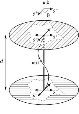
FIG. 1.: Sketch of a fluctuation of the bulk director field ${\bf n}({\bf r})$ (thin line) around its mean value $\hat{\bf z}$ (bold line). The two anisotropic plates impose a homeotropic anchoring (i.e., the preferred surface value of ${\bf n}$ is $\hat{\bf z}$) characterized by an anisotropic anchoring elasticity: deviations from $\hat{\bf z}$ are easier in the “soft” directions $\hat{\bf y}^{\pm}$ than in the “hard” directions $\hat{\bf x}^{\pm}$. In this geometry, the fluctuation-induced “Casimir” interaction between the plates depends both on their separation $d$ and their relative angle $\theta$.

“Casimir” effects arise from the quantization of the fluctuation modes by the boundaries (essentially from the suppression of modes of wavevector smaller than $2\pi/d$). The actual effect of the boundaries on a fluctuation mode of wavevector $q\simeq 2\pi/d$ is a function of the product $q\lambda$, where $\lambda$ is the extrapolation length corresponding to the considered polarization of the fluctuation. Depending on the relative values of $\lambda_{\rm min}$, $\lambda_{\rm max}$ and $d$, three different regimes occur: (i) For $\lambda_{\rm min}\ll\lambda_{\rm max}\ll d$ the constraints are effectively hard in both directions and the anisotropy is washed out at leading order. (ii) For $\lambda_{\rm min}\ll d\ll\lambda_{\rm max}$ the director field is subject to a hard constraint in the $x$ direction while it is virtually free in the (perpendicular) $y$ direction. (iii) Finally, for $d\ll\lambda_{\rm min}\ll\lambda_{\rm max}$ both directions allows almost free fluctuations and the anisotropy is lost again at leading order. To emphasize the effect of the anisotropy, we thus focus on the case where $\lambda_{\rm min}\ll d\ll\lambda_{\rm max}$.

Following Ref. [7], we now proceed to calculate the partition function for the director fluctuations, using ${\cal H}+{\cal H}_{s}$ as the total Hamiltonian. The quantum mechanical description of the partition function [7], which treats $z$ as an imaginary time variable, helps us gain a useful insight into the meaning of the boundary conditions. From the “imaginary time action” ${\cal H}$, one can define the “momentum” conjugate to a component of $\delta{\bf n}$ as $P_{\delta n}=K\,\partial_{z}\delta n$. Then, one can go from coordinate space to momentum space. In particular, at the boundaries one finds out that $P_{\delta n}$ is quadratically confined by the tensor ${\sf W}^{-1}$ and thus acts opposite as compared to $\delta n$. In other words, there is an uncertainty principle relating the fluctuations of $\delta n$ and $\partial_{z}\delta n$ as $\Delta(\delta n)\Delta(\partial_{z}\delta n)\simeq k_{\rm B}T/K$. In light of this, one can argue that the boundary condition of nearly free fluctuations in the soft direction is asymptotically equivalent to setting $\partial_{z}\delta n=0$. Note that this is equivalent to assuming that the directors cannot bear torques due to the freedom of rotation in the soft direction.

With the above justification, we can employ a somewhat less involved path integral formulation [1, 6] using the following boundary conditions: $\delta{\bf n}^{\pm}\cdot{\hat{\bf x}}^{\pm}=0$, $\partial_{z}\delta{\bf n}^{\pm}\cdot{\hat{\bf y}}^{\pm}=0$. The partition function of the fluctuating director field subject to the above constraints can be written as

$${\cal Z} = \int\!{\cal D}\delta{\bf n}({\bf r})\,\,\delta\{\delta{\bf n}^{-}\cdot{\hat{\bf x}}^{-}\}\,\delta\{\partial_{z}\delta{\bf n}^{-}\cdot{\hat{\bf y}}^{-}\}$$ (5)

$$\times\,\delta\{\delta{\bf n}^{+}\cdot{\hat{\bf x}}^{+}\}\,\delta\{\partial_{z}\delta{\bf n}^{+}\cdot{\hat{\bf x}}^{+}\}\,e^{-{\cal H}/{k_{\rm B}T}}.$$

The functional delta functions can be written as integral representations by introducing four Lagrange multiplier surface fields:

$${\cal Z} = \int\!{\cal D}\delta{\bf n}({\bf r})\,{\cal D}l_{1}({\bf r}_{\perp})\,{\cal D}l_{2}({\bf r}_{\perp})\,{\cal D}l_{3}({\bf r}_{\perp})\,{\cal D}l_{4}({\bf r}_{\perp})\,\,\exp\left\{-{\kappa\over 2}\int\!\!\!\int\!\!\!\int\!d^{3}{\bf r}\left[\nabla\delta{\bf n}({\bf r})\right]^{2}\right.$$ (7)

$$+\left.i\int\!\!\!\int\!d^{2}{\bf r}_{\perp}\left[l_{1}({\bf r}_{\perp})\,\delta{\bf n}^{-}({\bf r}_{\perp})\cdot{\hat{\bf x}}^{-}+l_{2}({\bf r}_{\perp})\,\partial_{z}\delta{\bf n}^{-}({\bf r}_{\perp})\cdot{\hat{\bf y}}^{-}+l_{3}({\bf r}_{\perp})\,\delta{\bf n}^{+}({\bf r}_{\perp})\cdot{\hat{\bf x}}^{+}+l_{4}({\bf r}_{\perp})\,\partial_{z}\delta{\bf n}^{+}({\bf r}_{\perp})\cdot{\hat{\bf y}}^{+}\right]\right\},$$

where $\kappa=K/k_{\rm B}T$. The integration over the director field is now Gaussian and can be easily performed. It yields

$${\cal Z}=\int\!{\cal D}l_{1}({\bf q}_{\perp})\,{\cal D}l_{2}({\bf q}_{\perp})\,{\cal D}l_{3}({\bf q}_{\perp})\,{\cal D}l_{4}({\bf q}_{\perp})\,\exp\left\{-\frac{1}{4\kappa}\!\sum_{\alpha,\beta=1}^{4}\!\int\!\!\!\int\!{d^{2}{\bf q}_{\perp}\over(2\pi)^{2}}\,l_{\alpha}(-{\bf q}_{\perp})\,M_{\alpha\beta}({\bf q}_{\perp})\,l_{\beta}({\bf q}_{\perp})\right\},$$ (8)

in which

$${\sf M}(q)=\left[\begin{array}[]{cccc}\displaystyle{1\over q}&0&\displaystyle{e^{-qd}\over q}\cos\theta&-e^{-qd}\sin\theta\\ \\ 0&-q&e^{-qd}\sin\theta&-qe^{-qd}\cos\theta\\ \\ \displaystyle{e^{-qd}\over q}\cos\theta&e^{-qd}\sin\theta&\displaystyle{1\over q}&0\\ \\ -e^{-qd}\sin\theta&-qe^{-qd}\cos\theta&0&-q\end{array}\right],$$ (9)

where $\theta$ is the angle between the corresponding soft axes of the two plates (see Fig. 1). The remaining integration over the Lagrange multiplier fields can be performed to give $\ln{\cal Z}=-{1\over 2}\sum_{{\bf q}_{\perp}}\ln\left(\det{\sf M}({\bf q}_{\perp})\right)$, which leads to a simple expression for the free energy per unit area:

$${\cal F}(\theta,d)={k_{\rm B}T\over 2\pi d^{2}}\int_{0}^{\infty}\!du\,u\,\ln\left[1-e^{-2u}\cos 2\theta\right].$$ (10)

Integration over $u$ then gives the final result Eq. (1) above. The function $f(\theta)=\sum_{k=1}^{\infty}{\cos^{k}(2\theta)/k^{3}}$ which describes the orientational dependence of the interaction has the structure of a zeta function that is commonly present in “Casimir” interactions.

It is instructive to examine the limiting cases of plates in which the corresponding hard and soft axes are parallel or perpendicular to each other. For $\theta=0$ the boundary conditions corresponds to a hard-hard configuration for one component of $\delta{\bf n}$ and a soft-soft one for the other. One can check that $f(0)=\zeta(3)\simeq 1.20206$ ($\zeta$ is the zeta function), thus we obtain exactly the same expression for the “Casimir” energy as in Ref. [7] for “alike” boundary conditions. On the other hand $f({\pi\over 2})=-{3\over 4}\zeta(3)$, which gives the same result as in Ref. [7] for “unlike” boundary conditions ($\theta=\pi/2$ corresponds to a soft-hard configuration for both components of $\delta{\bf n}$).

Our calculation suggests two kind of experiments: (i) a direct measure of the torque exerted between two plates at a fixed separation, and (ii) a measure of force as a function of separation for plates at various angles.

A possible experimental setup for the direct observation of the fluctuation-induced torque could be a torsion pendulum similar to the one discussed in Ref. [23]. Our results imply that the torsion coefficient of the pendulum $k$ (defined as the ratio between the torque $\tau$ and the angular rotation $\Delta\theta$) is corrected at $\theta=0$ by an amount

$$\Delta k={\pi^{2}\over 12}\times{k_{\rm B}TR^{2}\over d^{2}},$$ (11)

due to the “Casimir” effect. Here $R$ is the radius of the plates of area $\pi R^{2}$. Using the typical values $k_{\rm B}T=4.1\times 10^{-14}$ dyn cm, $R=1.5$ cm, $d=10^{-4}$ cm, one obtains $\Delta k\sim 10^{-5}$ dyn cm. This accuracy may be reachable using modern micro-manipulation techniques.

A measure of the force-distance relation for various angles $\theta$ could also be performed. An advantage of this procedure, as compared to measurement of the “simpler” effect corresponding to isotropic anchoring, is that relative effects are more easily detectable. Indeed, while the weak signal of the “Casimir” force can be swamped by stronger effects (Van der Waals, etc.), the difference between measurements performed at $\theta=0$ and $\theta=90^{\circ}$ should provide a differential evidence of the Casimir scaling.

We are grateful to R. Barberi, I. Dozov, P. Galatola and L. Peliti for invaluable discussions and comments. This research was supported in part by the National Science Foundation under Grant No. DMR-98-05833, and by ESPCI through a Joliot visiting chair for one of us (RG).

REFERENCES

- [1] For a review, see M. Kardar and R. Golestanian, Rev. Mod. Phys. 71, 1233 (1999).
- [2] M. Krech, The Casimir Effect in Critical Systems (World Scientific, Singapore, 1994).
- [3] V. M. Mostepanenko and N.N. Trunov, The Casimir Effect and Its Applications (Clarendon Press, Oxford, 1997).
- [4] H. B. G. Casimir, Proc. Kon. Ned. Akad. Wetenschap B 51, 793 (1948).
- [5] K. Symanzik, Nucl. Phys. B190, 1 (1981).
- [6] H. Li and M. Kardar, Phys. Rev. Lett. 67, 3275 (1991); Phys. Rev. A 46, 6490 (1992).
- [7] A. Ajdari, L. Peliti, and J. Prost, Phys. Rev. Lett. 66, 1481 (1991); A. Ajdari, B. Duplantier, D. Hone, L. Peliti, and J. Prost, J. Phys. II 2, 487 (1992).
- [8] D. Bartolo, D. Long and J.-B. Fournier. Europhys. Lett. 49, 729 (2000).
- [9] P. Ziherl, R. Podgornik, and S. Zǔmer, Phys. Rev. Lett. 82, 1189 (1999).
- [10] P. Ziherl, F. K. P. Haddadan, R. Podgornik, and S. Zǔmer, Phys. Rev. E 61, 5361 (2000).
- [11] M. Goulian, R. Bruinsma, and P. Pincus, Europhys. Lett. 22, 145 (1993).
- [12] R. Golestanian, M. Goulian, and M. Kardar, Europhys. Lett. 33, 241 (1996); Phys. Rev. E 54, 6725 (1996); R. Golestanian, Phys. Rev. E, 62, 5242 (2000).
- [13] P. G. Dommersnes and J.-B. Fournier. Europhys. Lett. 46, 256 (1999); Eur. Phys. J. B 12, 9 (1999).
- [14] F. Oosawa, Polyelectrolytes (Marcel Dekker, New York, 1971).
- [15] J.-L. Barrat and J.-F. Joanny, Adv. Chem. Phys. XCIV, 1 (1996).
- [16] R. Podgornik and V. A. Parsegian, Phys. Rev. Lett. 80, 1560 (1998).
- [17] B.-Y. Ha and A. J. Liu, Europhys. Lett. 846, 624 (1999).
- [18] P.-G. de Gennes and J. Prost, The Physics of Liquid Crystals (Clarendon, Oxford, 1993).
- [19] Note that similar ideas have been recently introduced in the case of electromagnetic quantum fluctuations by O. Kenneth and S. Nussinov, preprint hep-th/9802149; hep-th/0001045.
- [20] G. P. Bryan-Brown, C. V. Brown, I. C. Sage, and V. C. Hui, Nature 392, 365 (1998).
- [21] R. Barberi, private communication.
- [22] F. C. Frank, Discuss. Faraday Soc. 25, 19 (1958).
- [23] S. Faetti, M. Gatti, and V. Palleschi, J. Physique Lett. 46, L-881 (1985).