0pt0.4pt
Susceptibility and Percolation in 2D Random Field Ising Magnets
Abstract
The ground state structure of the two-dimensional random field Ising magnet is studied using exact numerical calculations. First we show that the ferromagnetism, which exists for small system sizes, vanishes with a large excitation at a random field strength dependent length scale. This break-up length scale scales exponentially with the squared random field, . By adding an external field we then study the susceptibility in the ground state. If , domains melt continuously and the magnetization has a smooth behavior, independent of system size, and the susceptibility decays as . We define a random field strength dependent critical external field value , for the up and down spins to form a percolation type of spanning cluster. The percolation transition is in the standard short-range correlated percolation universality class. The mass of the spanning cluster increases with decreasing and the critical external field approaches zero for vanishing random field strength, implying the critical field scaling (for Gaussian disorder) , where and . Below the systems should percolate even when . This implies that even for above the domains can be fractal at low random fields, such that the largest domain spans the system at low random field strength values and its mass has the fractal dimension of standard percolation . The structure of the spanning clusters is studied by defining red clusters, in analogy to the “red sites” of ordinary site-percolation. The size of red clusters defines an extra length scale, independent of .
PACS # 05.50.+q, 75.60.Ch, 75.50.Lk, 64.60.Ak
I Introduction
The question of the importance of quenched random field (RF) disorder in ferromagnets traces back to the primary paper by Imry and Ma [1, 2] from mid-seventies. They argued using energy minimization for an excitation to the ground state, that the randomness in the fields assigned to spins changes the lower critical dimension from the pure case with to . After that a number of field-theoretical calculations suggested that the randomness increases with two to be . Finally came rigorous proofs first by Bricmont and Kupiainen [3] in ’87 that there is a ferromagnetic phase in the three-dimensional (3D) random field Ising model (RFIM) and in ’89 by Aizenman and Wehr [4] that there is no ferromagnetic phase in 2D RFIM. Thus it was established that the lower critical dimension is two. This means that the ground state is a paramagnet, but the problem as to how to describe the structure of the (ground state of) 2D RFIM still persists. Some recent work concerns the scaling of the correlation lengths [5] and there is a suggestion of a ferromagnetic phase, but with a magnetization that is in the thermodynamic limit below unity [6]. The point is that due to the (relevant) disorder there are no easy arguments that would indicate, say, how the paramagnetic ground state should be characterized. This is different from the thermal Ising case, which is quite trivial in 1D.
In two dimensional Ising magnets, in the presence of quenched random fields, the problem of determining the ground state (GS) becomes more difficult. Finding the true ground state with any standard Monte Carlo method is problematic due to the complex energy landscape. Even with the exact ground state methods, as the one used in this paper, the thermodynamic limit is difficult to reach, since the finite size effects are strong. In the typical case of square lattices the only way not to have a massive domain, which would scale with the Euclidean dimension of the system, is to have enough interpenetrating domains of both spin orientations. However, with decreasing strength of the randomness the ferromagnetic coupling constants between spins start to matter, the domains become “thicker”, and thus one enters an apparent ferromagnetic regime, and the paramagnetic (PM) phase is encountered only at very large length scales. Should there be large clusters with a fractal (non-Euclidian) mass scaling they nevertheless can contribute to the physics in spite of the fact that the total fraction of spins can be negligible in the thermodynamics limit. Thus such clusters may even be measurable in experiments or be related to the dynamical behavior in non-equilibrium conditions. Therefore it is of interested to study the structure of the large(st) clusters in the ground state, since it is not simply paramagnetic like in normal Ising magnets above . The true ground state structure gives also some insight into the physics at , since the overlap between the GS and the corresponding finite- state is close to unity for small, in contrast to the thermal chaos in spin glasses [7].
In this paper we want to shed some light on the character of the ground states of 2D RFIM. We have done extensive exact ground state calculations in order to characterize how the ferromagnetic (FM) order vanishes with increasing system size. We have also studied the effect of the application of an external field, that is the susceptibility of the 2D RFIM. Allowing for a non-zero external field makes it possible to investigate a percolation -type of critical phenomenon for the largest clusters. We propose a phase diagram in the disorder strength and external field plane for the percolation behavior. The presence of clusters of the size of the system, i.e. percolation type of order brings another correlation length in the systems and thus makes the decay of ferromagnetic order more complicated than at first sight.
The Hamiltonian of the random field Ising model is
| (1) |
where (in this paper we use for numerical calculations) is the coupling constant between nearest-neighbor spins and . We use here square-lattice. is a constant external field, which if non-zero is assigned to all of the spins, and is the random field, acting on each spin . We consider mainly a Gaussian distribution for the random field values
| (2) |
with the disorder strength given by , the standard deviation of the distribution, though in some cases the bimodal distribution,
| (3) |
is used, too. The results presented below should not be too dependent on the actual , in any case.
To find the ground state structure of the RFIM means that the Hamiltonian (1) is minimized, in which case the positive ferromagnetic coupling constants prefer to have all the spins aligned to the same direction. On the other hand the random field contribution is to have the spins to be parallel with the local field, and thus has a paramagnetic effect. This competition of ferromagnetic and paramagnetic effects leads to a complicated energy landscape and the finding the GS becomes a global optimization problem. An interesting side of the RFIM is that it has an experimental realization as a diluted antiferromagnet in a field (DAFF). By gauge-transforming the Hamiltonian of DAFF
| (4) |
where the coupling constants , is the occupation probability of a spin , and is now a constant external field, one gets the Hamiltonian of RFIM (1) with [8, 9, 10]. The ferromagnetic order in the RFIM corresponds to antiferromagnetic order in the DAFF, naturally.
As background, it is of interest to review a few basic results. Imry and Ma used a domain-wall argument to show that the lower critical dimension [1]. In order to have a domain there is an energy cost of from the domain wall. On the other hand the system gains energy by flipping the domain from the fluctuations of random fields, which interpreted as a typical fluctuation means that the gain is . Thus, whenever , i.e. , it is energetically favorable for the system to break into domains. However, in this paper we will point out, as it has been shown in 1D [11], that the scaling can be used only in relation to the sum of the random fields in the “first excitation”, but not to the droplet field energy when the GS consists of domains of different length scales.
Grinstein and Ma [12] derived from the continuum interface Hamiltonian that the roughness of the domain wall (DW) in RFIM scales as , which is consistent with . Later Fisher [13] used the functional renormalization group (FRG) to obtain the roughness exponent and argued that due to the existence of many metastable states the perturbative RG calculations and dimensional reduction fail. Another, microscopic calculation by Binder [14] optimized the domain-wall energy in two-dimensions. The net result is a total energy gain from random fields, due to domain wall decorations, which implies that the domain wall energy vanishes on a minimal length scale
| (5) |
where is a constant of order unity. For the expectation is that the system spontaneously breaks up into domains. Similarly the energy of a domain with a constant external field becomes
| (6) |
Setting and assuming that the critical length scale scales as , without the field, i.e. , the critical external field becomes
| (7) |
Note, that in this case the first two terms in (6) assume that the domain is compact.
These results imply, together with the notion that the ground state is paramagnetic, that the magnetization should not as such display any “universal” features. The results of this paper show that the magnetization is not dependent on the system size and has a smooth behavior of and the susceptibility vanishes with the system size as , where const, and . These imply that there is a length scale, related to the rate at which clusters “melt” when is changed from zero.
The presence of such a length scale is qualitatively similar to the one discovered in the context of the percolation transition. It turns out so that when the external field is varied, the universality class is that of the ordinary short-range correlated percolation universality class. The external field threshold for spanning with respect to decreasing random field strength approaches zero external field limit from the site-percolation limit of infinite random field strength value, suggesting a behavior for Gaussian disorder of , where and . Below this value the lattice effects of site percolation are washed out, and there is yet another length scale that characterizes the percolation clusters, the size of the “red clusters” defined below in analogy to the usual red or cutting sites in percolation. Now a whole cluster is reversed due to the forced reversal of a “seed” cluster, when the sample is optimized again. The length scale is however finite, indicating that the global optimization of the ground state creates only finite spin-spin correlations as is the case in 1D as well.
This paper is organized so that it starts by introducing in Section II the exact ground state calculation technique. In Section III the breaking up of ferromagnetic order is discussed, based on a nucleation of droplets -picture which follows from a level crossing between a FM ground state and one with a large droplet. The relevant scaling (5) is derived from extreme statistics. Above the break-up length scale the domains have a complex structure that is briefly discussed. The effect of an external field, in the case the system size is above , is studied in Section IV for Gaussian disorder. The percolation aspects of the 2D RFIM are studied in detail in Section V. The phase diagram for the percolation behavior as functions of the external field and the random field strength is sketched and the properties of the transition are discussed. The zero-external field percolation probability is studied in Section VI. In the section also the structure of spanning clusters is studied using the so called red clusters whose scaling and properties are discussed. The paper is finished with conclusions in Section VII.
II Numerical Method
For the numerical calculations the Hamiltonian (1) is transformed to a random flow graph with two extra sites: the source and the sink. The positive field values correspond flow capacities connected to the sink () from a spin , similarly the negative fields with are connected to the source (), and the coupling constants between the spins correspond flow capacities from a site to its neighboring one [15]. In the case the external field is applied, only the local sum of fields, , is added to a spin towards the direction it is positive. The graph-theoretical combinatorial optimization algorithms, namely maximum-flow minimum-cut algorithms, enable us to find the bottleneck, which restricts the amount of the flow which is possible to get from the source to the sink through the capacities, of such a random graph. This bottleneck, path which divides the system in two parts: sites connected to the sink and sites connected to the source, is the global minimum cut of the graph and the sum of the capacities belonging to the cut equals the maximum flow, and is smaller than of any other path cutting the system. The value of the maximum flow gives the total minimum energy of the system. The maximum flow algorithms are proven to give the exact minimum cut of all the random graphs, in which the capacities are positive and with a single source and sink [16]. In physical situations this means the systems are without local frustration. The algorithm was actually used for the first time in this context by Ogielski [17], who showed that the 3D RFIM has a ferromagnetic phase. The best known maximum flow method is by Ford and Fulkerson and called the augmenting path method [18]. We have used a more sophisticated method called push-and-relabel by Goldberg and Tarjan [19], which we have optimized for our purposes. It scales almost linearly, , with the number of spins and gives the ground state in about minute for a million of spins in a workstation.
When we have added an external field in the systems our system sizes are restricted to , for small but nonzero due to the range of integer variables (for numerical reasons we use a discrete representation of real fields). When the high precision for field values is not needed the computations extend up to system sizes . We have used periodic boundary conditions in all of the cases. Also the percolation is tested in the periodical or cylindrical way, i.e., a cluster has to meet itself when crossing a boundary in order to span a system.
When the red clusters are studied, Section VI C, we have applied a technique, which allows us to take advantage of the so called residual graph [20]. After the original ground state is searched a perturbation is applied. This means that e.g., a spin is forced to be to the other direction with a large opposite field value. Then the ground state is searched again. This time all the flow need not to be constructed from scratch, but instead one can utilize the final situation of the first ground state search (the residual graph). Only the extra amount of flow, needed since the capacity of the large opposite field value is added, has to be forced through the system to the sink. One has to subtract also the flow from the original field value (retrace it back to the source). It is thus convenient to reverse only the fields which originally were negative. For the positive field values one would have to study a mirror copy of the system (). Thus we have analyzed the red clusters only from the spanning clusters of down spins, which does not disturb the statistics, since the spin directions are symmetrical. The use of the residual graph reduces the time to calculate the next ground state considerably, although approximately a half of the spanning clusters have to be neglected. Notice that since the ground state energy is a linear function of the capacity of the saturated bonds (or the field of the spins aligned along the local field) one can compute the “break-point” field , at which a change takes place from the original ground state to the new one. We have not paid attention to this, however, due to our main interest in the geometry of the red clusters. One interesting additional question would be what is the smallest and its disorder-averaged distribution.
III Destruction of ferromagnetic order
In this section we will derive the scaling for the break-up length scale , Eq. (5), from extreme statistics (as done in the paper by Emig and Nattermann [21]). and confirm it with exact ground state calculations. We also discuss the ensuing domain structure qualitatively.
If one picks a (compact) subregion of area of a ferromagnetic 2D RF system the energy is drawn from a Gaussian distribution
| (8) |
where the variance is due to the fluctuations of random fields, and . For a system of size we have ways of making such a subregion. The probability that a subregion has the lowest energy is given by
| (9) |
where [22]. The distribution is in fact a Gumbel distribution [23]. The average value of the lowest energies is given by
| (10) |
which can not be solved analytically. The typical value of the lowest energy follows from an extreme scaling estimate. The factor inside the curly brackets in (9) is close to unity if becomes small enough (for similar applications, see [24, 25, 26, 27]). Thus
| (11) |
which yields,
| (12) |
i.e. the energy gain from the fluctuations is
| (13) |
A FM system would tend to take advantage of such large favorable energy fluctuations by reversing a domain, which requires breaking bonds. This is assumed to have a cost of
| (14) |
Equating Eqs. (13) and (14) yields the estimate of the parameter values at which the first “Imry-Ma” domain occurs,
| (15) |
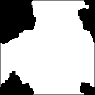
It can be easily understood that the most preferable domain is the one, which maximizes the area and minimizes the bonds to be broken, which gives . Fig. 1 illustrates this, as we increase (with a fixed random field configuration and system size) the strength of the randomness or decrease the ferromagnetic couplings until the first domain appears. It turns out to be so that the droplet is of the order of the system size. This kind of nucleation with a critical size is reminiscent of a first order transition, and is related to a level-crossing, when either the random field strength or the system size is varied, similarly to random elastic manifolds, when an extra periodic potential [25] or a constant external field [26] is applied. By substituting and to (15), we get for the length scale
| (16) |
which is in fact as in (5). This result, (16), is surprising in the sense, that the extreme statistics calculation for the formation of a domain leads to the exactly same scaling as the optimization of a domain wall energy on successive scales in Binder’s argument.
Due to the extensive size of the first domain-like excitation the destruction of the ferromagnetism resembles a first order transition. The magnetization for a certain disorder strength and system size would be averaged over systems, in which the excitation has and has not been formed yet, with and , respectively. Hence we define a simpler measure for the break up of FM order: the probability of finding a purely ferromagnetic system, , i.e., for a fixed random field strength and system size we calculate the probability over several realizations that magnetization [28]. If the transition to the PM state would be continuous, this would not make much sense, since already small fluctuations would cause . However, due to the first order behavior, and to the fact that the smallest energy needed to flip a domain causes the excitation to be large, is a good measure and has a smooth behavior. We have checked that vs. does not depend on .
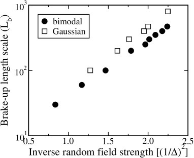
We have derived the break-up length scale by varying the random field strength from the probability of finding a pure ferromagnetic system as . The data is shown in Fig. 2 for Gaussian and bimodal disorder (in both cases ), and the exponential scaling for vs. inverse random field strength squared is clearly seen. The prefactors are and for Gaussian and bimodal disorder, respectively. To check that the probability is not due to so called stiff spins, i.e., single spins for which , we next derive an extreme statistics formula for their existence. The probability of finding . The extreme statistics argument, , with , gives
| (17) |
For Gaussian for which in Fig. 2 from Eq. (17). also grows much faster than for decreasing which is both easy to see from Eq. (17) and to check numerically. For for which becomes as huge as 22300. To confirm further that the origin for the break-up is a large domain, one can extend the argument to small domains. The length scale at which one is able to find a cluster of two neighboring spins flipped, i.e., , where , , becomes even greater than . These small clusters are present in large system sizes, but do not play a role in the probability of first excitation, since the energy minimization prefers extensive domains. It is amusing to note that the critical droplet size reminds of critical nucleation in ordinary first order phase transitions. It is also worth pointing out that the reasoning for stiff spins does not work for the bimodal distribution (since it is bounded), and indeed we observe as expected a similar scaling for both the Gaussian and bimodal disorders.
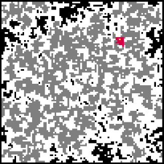
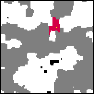
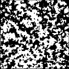
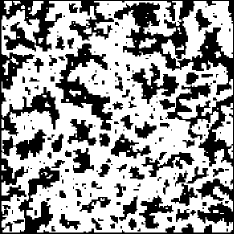
When a system size is well above the break-up length scale the Imry-Ma argument is no longer applicable to the structure. In Fig. 3 we depict two systems with a large Gaussian random field strength value and with a smaller one for a system size . One can see that a system breaks to smaller and smaller domains inside each other from the case seen in Fig. 1. The feature of having clusters in different scales is familiar from the percolation problem [29]. In fact in both of the examples in Fig. 3 there is a domain, which spans the system in vertical direction, drawn in gray. For the stronger random field value one can see also smaller domains of different sizes. However, the width of the spanning cluster is greater than in a standard site or bond occupation percolation problem. Later in subsection VI B we discuss the scaling properties of the largest clusters in the ground state, above .
IV Magnetization and susceptibility with an external field
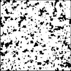
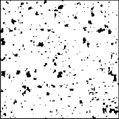
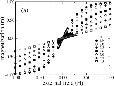
In Fig. 4 we show what happens in system, with a system size well above when an external field is applied. Now the clusters “melt” smoothly when the external field strength is increased and such first order type of phenomenon is not seen as when a first Imry-Ma droplet appears in the zero-field case. The magnetization has a continuous behavior, see Fig. 5(a), where we have the magnetization with respect to the external field for several Gaussian disorder strength values. All the magnetization values for different system sizes lie exactly on top of each other, when , and as long as the statistics is good.
For smaller system sizes one could study “avalanche”-like behavior, i.e. the sizes of the areas that get turned with the magnetic field (see [30]). However, these are due to the first order break-up, defined by (7) and one should bear in mind that such behavior does not exist in the thermodynamic limit, , when the system sizes are above the break-up length scale. For our results indicate that the size distribution of the flipped regions as is swept is not that interesting.
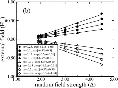
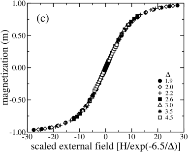
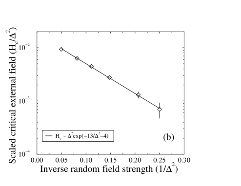
In order to find the scaling between the external field and the random field strength we have taken from Fig. 5(a) the crossing points of magnetization curves with a fixed magnetization values at external fields for different random field strength values . The external field scales exponentially with respect to the random field strength,
| (18) |
see Fig. 5(b). This is also an evidence of non-existence of a critical point in , in which case there should be a power-law behavior if the transition was continuous, thus no PM to FM transition is seen. The data-collapse using the scaling (18) is shown in Fig. 5(c) confirming the prediction of the scaling. The magnetization has a linear behavior with respect to the external field for small field values and exponential tails. The exponential behavior of Eq. (18) implies that there is a unique “melting rate” at which the cluster boundaries get eroded as increases and that the process is otherwise similar for all . We have no analytical argument for the melting rate [or the slope of the -curve], and note that it is not seemingly, at least, related to .
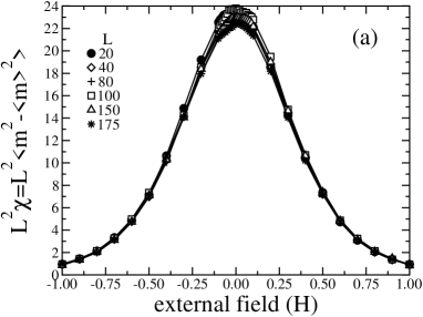
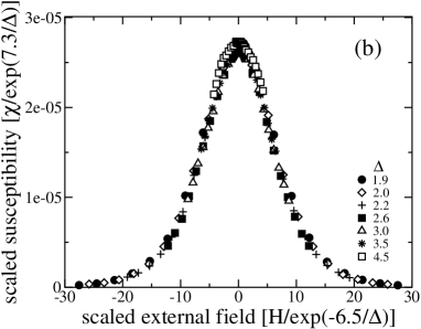
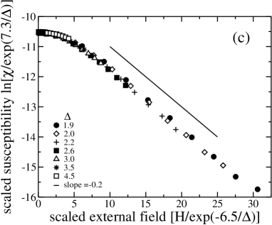
We have also studied the susceptibility, , with respect to the external field. In Fig. 6(a) the susceptibility is shown for a fixed random field strength and varying system size. The data has been collapsed with the area of the systems, . In Fig. 6(b) we have data-collapsed the susceptibility versus random field strength by scaling the external field with (18) as for magnetization and the susceptibility with . Again the exponential behavior is a sign of non-existence of any critical point, due to the lack of power-law divergence at any . Although the shape of the data-collapse of the susceptibility looks almost Gaussian, it is actually not. It has a constant value for small external field values and exponential tails for large values, as seen in Fig. 6(c). This results straightforwardly from the magnetization, since . To summarize the behavior of the susceptibility, it is
| (19) |
where is from Eq. (18) and
| (20) |
Therefore the fluctuations of the magnetization are associated with yet another scale, which is almost but not quite an inverse of that related to the magnetization. From the suscpetibility one gets the magnetization correlation length , which has an exponential dependence on the random field strength. It should be noted, finally, that we have here studied only the case with Gaussian disorder. With any other distribution we would expect that the prefactors in Eqs. (18), (19), and (20) would change.
V Percolation with an external field
Motivated by Fig. 3, where the domains resemble the percolation problem we next study the percolation behavior in the 2D random field Ising magnets with Gaussian disorder. The usual bimodal distribution could be studied as well, but since it is susceptible to some anomalous features we concentrate on the Gaussian case which does not have these problems. The bimodal case suffers from the fact that the ground states are highly degenerate at fractional field strength values. Thus there are some ambiguities in how define percolation clusters [31, 32].
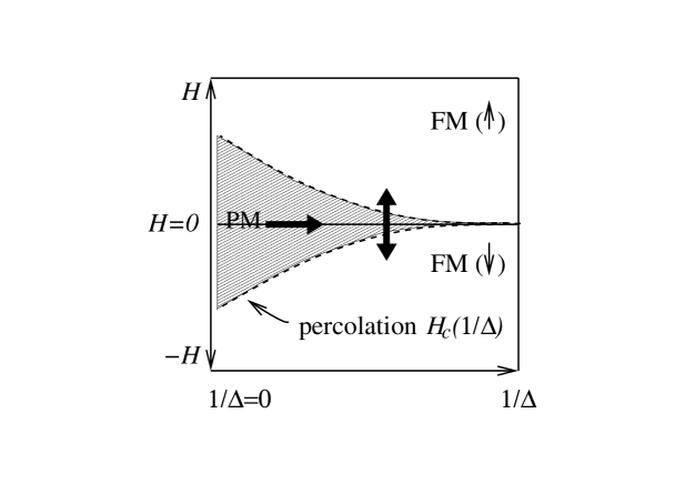
When the random field strength is well above the coupling constant value, , the percolation can be easily understood by considering it as an ordinary site-occupation problem. This means that, only the random field directions are important and the coupling constants may be neglected. The site-percolation occupation threshold probability for square-lattices is [29], i.e., well above one half. Applied to the strong random field strength case it means that there must be a finite external field in order to get a domain spanning the system. However, when the random field strength is decreased, the coupling constants start to contribute and in some cases systems span even without an external field, as in Fig. 3. Hence, we propose a phase-diagram Fig. 7. There we can take the limit so that the ordinary site-percolation problem is encountered. This is true for distributions for which one can control the fraction of “stiff” spins (i.e. ) systematically. In the case of Gaussian disorder there will be of course, even for very large a small fraction of “soft” spins where this criterion is not fulfilled. Thus the exact point that the percolation line approaches in the -limit will depend on the distribution, but we expect that the “” is different from one-half, that is . Notice that again the binary distribution presents a problem.
When the percolation threshold lines start to approach each other and the line. Now there arises two questions. The first one is, what kind of a transition is the percolation here? Is it like the ordinary short-range correlated percolation, suggested by the site-percolation analogy for the strong random field strength case, or are there extra correlations due to the global optimization relevant here? Examples about similar cases can be found from Ref. [33]. The second question is, do the lines meet each other at finite , i.e. does there exist a spanning cluster also when and ? Our aim is to answer these two questions in this section, where we study the percolation problem in the vertical direction in the phase-diagram Fig. 7, and in the next section, where the horizontal direction, line, is considered.
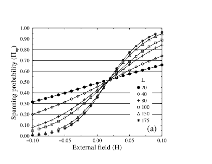
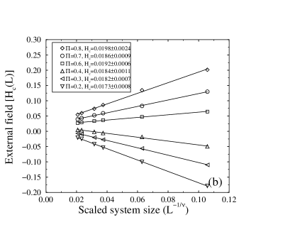
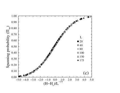
In Fig. 8(a) we have drawn the spanning probabilities of up spins with respect to the external field for several system sizes , which are greater than , for a fixed random field strength . The curves look rather similar to the standard percolation. When we take the crossing points of the spanning probability curves with fixed spanning probability values for each systems size , we get an estimate for the critical external field using finite size scaling, see Fig. 8(b). There we have attempted successfully to find the value for using the standard short-range correlated 2D percolation correlation length exponent . Using the estimated for we show a data-collapse of versus in Fig. 8(c), which confirms the estimates of and [29]. We get similar data-collapses for various other random field strength values as well. In order to test further the universality class of the percolation transition studied here, we have also calculated the order parameter of the percolation, the probability of belonging to the up-spin spanning cluster . Using the scaling analysis for the correlation length
| (21) |
and for the order parameter, when ,
| (22) |
we get the limiting behaviors,
| (23) |
and thus the scaling behavior for the order parameter becomes
| (24) | |||
| (25) |
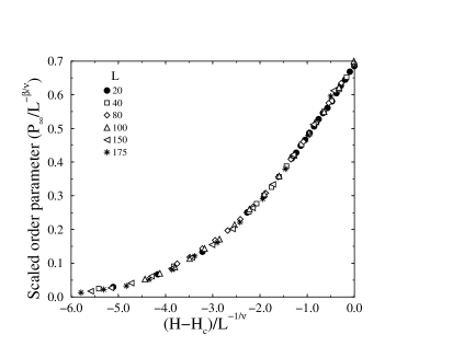
We have done successful data-collapses, i.e. plotted the scaling function , for various using the standard 2D short-range correlated percolation exponents and , of which the case with is shown in Fig. 9. Note, that the values are not shown, since cut-offs appear, due to the fact that is bounded in between and the non-scaled values after scaling saturate at different levels depending on the system size.
Hence, we conclude that the percolation transition for a fixed versus the external field is in the standard 2D short-range correlated percolation universality class [29]. This is confirmed by the fractal dimension of the spanning cluster, too, as discussed below. Also other exponents could be measured, as for the average size of the clusters, and and for the cluster size distribution. Note, however, that then the control parameter should be the external field instead of the disorder strength . See Ref. [34] for an example of the cluster size distribution for a non-critical case (, but ). The other exponents should be measurable, too, like the fractal dimension of the backbone of the spanning cluster, the fractal dimension of the chemical distance, the hull exponent etc. In addition to the correct control parameter also the break-up length scale, has to be considered, too. Notice that there is an slight contradiction hidden in the notion that the hull exponent could be measured. Namely, both the work of Ref. [34] and studies of domain walls enforced with appropriate boundary conditions give no evidence thereof. It seems likely that to recover the right exponent (4/3) one has to resort to studying the spanning cluster geometry itself at the critical point with . It is amusing to note that the standard 2D percolation hull exponent can be recovered in non-equilibrium simulations of 2D RFIM domain walls [35].
We have now shown, that there exists a line of critical external field values for percolation. The corresponding correlation length diverges as (21) with a correlation length exponent . On the other hand it was shown in the previous section, that there is no critical external field value for the magnetic behavior, i.e., no PM to FM transition, and the magnetic correlation length has an exponential dependence on . The percolation correlation length may cause some confusion, when studying the PM structure of the GS, since it brings in another length scale.
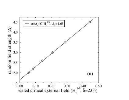
To answer the question how the percolation critical external field behaves with respect to the random field, we have attempted a critical type of scaling using the calculated for various 2.0, 2.2, 2.6, 3.0, and 4.5. For smaller becomes large and approaches the vicinity of zero, being thus numerically difficult to define. We have been able to use the Ansatz behavior of
| (26) |
where . In Fig. 10(a) we have plotted the calculated values versus the scaled critical external field and it gives the estimate for . This indicates that the percolation probability lines for up and down spins meet at and for below the critical there is always in the systems spanning of either of the spin directions, even for . Actually one should note, that the only way that neither of the spin directions span is to have a so called checker-board situation, which prevent both of the spin directions to have neighbors with the same spin orientation. However, the another scenario with an exponential behavior for fits also reasonably well. This would suggest, that there is no finite . Fig. 10(b) shows a behavior of . This can be compared with Eq. (7), where the break-up external field was derived. Notice that the derivation was for compact domains and the spanning clusters here are by default fractals. Besides that, the factor 13 in front of is much larger than in the scaling form for . The difference implies that the , at which length scale the spanning probability vanishes, scales as . The is already exponentially large length scale for small , so should be large enough that one can be below it in experiments, and thus a system can “apparently percolate” [36, 10].
VI Percolation at
To understand how the percolation transition is seen when there is no external field and the random field strength is changed we study the phase diagram in Section VI A in the direction of the horizontal arrow in Fig. 7. The structure of the spanning clusters are studied in Sections VI B and in VI C with the help of the so called red clusters.
A Spanning probability
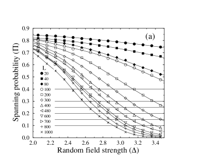
In Fig. 11(a) we have plotted the probability for spanning of either up or down spins as a function of the Gaussian random field strength . The probabilities are calculated up to , but only the interesting part of the plot is shown. There is a drop from at , which corresponds for each system size, to a value about . We have also calculated the in this case and it is approximately one half of . For the larger random field strength values the probabilities decrease and the lines get steeper, when the system size increases. In order to see, if the spanning probabilities are converging towards a step function at some threshold value, we have calculated the probabilities up to the system size and each point with 5000 realizations.
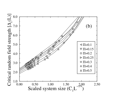
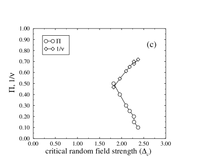
For each system size we have searched the crossing points of the spanning probability curves in Fig. 11(a) with fixed probability values 0.1, 0.15, 0.2, 0.25, 0.3, 0.4, and 0.5. Using finite size scaling for of the form we have estimated for each value, see Fig. 11(b). There we have plotted the versus the scaled system size . One sees that the different threshold values for spanning probabilities approach different critical random field strength values . The threshold ’s have been plotted with respect to in Fig. 11(c). In the ordinary percolation, this should be a step function, and the correlation length exponent independent on the criterion . However, here also is dependent on the criterion and varies with respect to . We believe, that this surprising phenomenon is due to that we are approaching the part in the phase diagram Fig. 7, where the percolation lines of up and down spins are getting close to each other. In terms of the two control parameters and one can think about the “percolation manifold”: it has a line of unstable fixed points . Usually is a good control parameter close to . Having as a control parameter seems to have the problem that one moves almost parallel to the actual line .
When considering the percolation probability of up or down spins, it actually consists of probabilities of up-spin spanning and down-spin spanning as , since they are correlated with each other. Assuming that (and respectively) has a value about one-half at the critical line of percolation at the thermodynamic limit, we get . In standard percolation such a value is not actually universal (and we have not confirmed it) but depends on the boundary conditions, etc. [37]. However, whatever the values for and are at the thermodynamic limit, as long as they are below unity, is below unity, too. This may be the reason, why there is an immediate drop in Fig. 11(a) from at for each system size, to a value about . If we approximate with a linear behavior the versus in Fig. 11(c), the critical value estimated in the previous section , when the percolation threshold for up-spin spanning, has a value about . Another interesting point in Fig. 11(c) is that the is about 3/4 , when versus approaches zero. Thus the standard correlation length exponent would be reached far enough away from the area, where the percolation threshold lines for up and down spins touch each other.
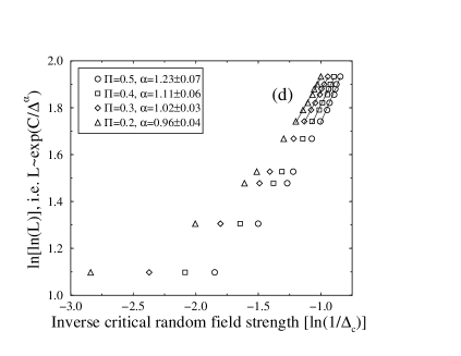
In order to test the break-up length scale type of scaling for the percolation behavior (5), we have taken from Fig. 11(a) the estimated for various values and plotted the system sizes in double-logarithm scale versus the logarithm of the inverse of the critical , see Fig. 11(d). The exponent, which is in scaling, , is now dependent on again. At least this does not solve the problem here, and the break-up length scale type of scaling can be ruled out.
B The percolation cluster
In order to see if the thickness of the spanning cluster affects the scaling of the standard percolation we have measured the fractal dimension of the spanning cluster when . By now unsurprisingly, the standard two-dimensional short-range correlated percolation fractal dimension fits very well in the data, as can be seen in Fig. 12. The least-squares fit gives a value of . We have measured also the sum of the random fields in the spanning cluster and found that the sum scales with the exponent , too. This is in contrast to the Imry-Ma domain argument, where the sum is taken scale as . The prefactor for the scaling of the sum of the random fields approaches slowly zero with decreasing random field strength, opposite to the mass of the spanning cluster, which increases with decreasing .
Hence, the Imry-Ma argument defines only the first excitation, and is irrelevant when it comes to domains when the system has broken up to many clusters on different length scales. Then the structure is due to a more complicated optimization. The domains are no longer compact and as noted above for large enough domains the domain-wall length should be characterized by the percolation hull exponent.
C Red clusters
So far all the evidence points out to the direction that the percolation transition is exactly of the normal universality class. To further investigate the nature of the clusters in the presence of the correlations from the GS optimization, we next look at the so-called red clusters. The structure of a standard percolation cluster can be characterized with the help of the “colored sites” picture in which one assesses the role of an element to the connectivity of the spanning cluster. This picture has been also called the links-nodes-blobs model with dead-ends [29]. The red sites, or links and nodes, are such that removing any single one breaks up the spanning cluster.
To compare with the original ground state we investigate what happens if one inverts, by fixing the local field to a large value opposite to the spin orientation, any spin belonging to the spanning cluster. Then the new GS is found with this change to the original problem. The effect is illustrated in Fig. 3, the crucial difference to site-percolation is that now a whole sub-cluster can be reversed. The spin drawn in yellow is the inverted, “seed” spin in the spanning cluster, and the spins painted red form the rest of the red cluster, which are flipped from the original ground state when the energy is minimized the second time. We do the investigation whether the original cluster retains its spanning property for each spin or trial cluster in analogy with ordinary percolation. Those spins that lead to a destructive (cluster) flip, define then red clusters (RC) as all the spins that reversed simultaneously.
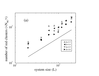
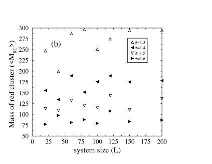
The finite size scaling of the number of the red clusters, , is shown in the Fig. 13(a) for different field values. is in practice calculated as the number of the seed spins, which cause the breaking of the spanning cluster, since two different seed spins may both belong to the same red clusters without the red clusters being identical. The technique to find the red clusters was introduced in Section II and although it is efficient, only up to the system size can be studied, since each of the spins in spanning clusters has to be checked separately, because one cannot know beforehand, whether it is critical or not - this is what we want to find out. For smaller field values the spanning cluster is “thicker” and the red clusters get larger. One can see from the Fig. 13(a) that scales with , where as in ordinary percolation, for field values , when . The amplitude is larger the smaller the field, as is the average mass of red clusters . is independent of the system size and depends only on the field , see Fig. 13(b).
The other elements of the spanning cluster, dead-ends and blobs, could be generalized, too. Here blobs, which are multiple connected to the rest of the spanning cluster, are such that in order to break a spanning cluster, several seed spins are needed to flip simultaneously instead of a single one. Links, nodes, and blobs form together the backbone of the spanning cluster, and the rest of the mass of the cluster is in the dead-ends. The red cluster size scale defines the average smallest size of any element of the spanning cluster.
VII Conclusions
In this paper we have studied the character of the ground state of the two-dimensional random field Ising magnet. We have shown that the break-up of the ferromagnetism, when the system size increases, can be understood with extreme statistics. This length scale has been confirmed with exact ground state calculations. The change of magnetization at the droplet excitation is naturally of “first-order” -kind.
Above the break-up length scale we have studied the magnetization and susceptibility with respect to a constant external field. The behavior of the magnetization and the susceptibility is continuous and smooth and does not have any indications of a transition or a critical point, in agreement with the expectations of a continuously varying magnetization around , and a paramagnetic ground state. We thus conclude that the correct way of looking at the susceptibility is to study it with respect to the external field and above the break-up length scale instead of as a function of the random field strength, when the first order character of the break-up length scale may among others cause problems.
However, we are able to find another critical phenomenon in the systems, in their geometry. For square lattices sites do not have a spanning property in ordinary percolation, when the occupation probability is one half. This corresponds to the random field case with high random field strength value without an external field. When an external field is applied and the random field strength decreased, a percolation transition can be seen. The transition is shown to be in the standard 2D short-range correlated percolation universality class, when studied as a function of the external field. Hence, the correlations in the two-dimensional random field Ising magnets are only of finite size. We also want to point out that in these kind of systems, the random field strength is a poor control parameter and the systems should be studied with respect to the external field, and after that map to the random field strength. By doing so we have been able to find a critical random field strength value, below which the systems are always spanning even without an external field. When the percolation transition is studied without an external field and tuning the random field strength lots difficulties are encountered. This might cause puzzling consequences when studying the character of the ground states, not only because of the bad control parameter, but also because the percolation correlation length may be mistaken for something as the magnetization correlation length. Also note that the “true behavior” is seen only for system sizes large enough ().
The percolation character of the ground state structure can be measured by the standard percolation fractal dimensional scaling for the mass of the spanning domain. The existence of such a large cluster is not against the paramagnetic structure of the ground state, since the fractal dimension is below the Euclidean dimension. In order to be consistent with the Aizenman-Wehr argument in the zero-external field limit the spins in the opposite direction from the external field may form the spanning cluster at low random field strength values. In fact we have found cases of finite systems for , where the magnetization of the system is opposite to the orientation of spins in the spanning cluster. Notice that this does not imply that the critical lines actually cross each other at continuing on the opposite side of the -axis (see Fig. 7). By considering the red clusters it seems that in the TD-limit the spanning cluster should be broken up at , since the field needed to flip such a critical droplet should go to zero with . Also, since the sum of the fields in the spanning cluster is shown to scale with the same fractal dimension as the mass, we conclude that the Imry-Ma argument does not work any more after the system has broken up on several domains. It works only for the first domain to appear.
We have also generalized the red sites of the standard percolation to red clusters in the percolation studied here. A red cluster results from the energy minimization by flipping a whole cluster although only a single spin has been forced to be flipped, and breaks up the spanning character of a percolating cluster. Actually the finite size of the red clusters indicate also the presence of only short-range correlations in the systems. Such a lack of long-range correlations maybe explains, why we can see an “accidental” percolation phenomenon in a zero-temperature magnet whose physics is governed by the disorder configuration. The normal percolation universality class is tightly connected to conformal invariance, which is most often destroyed by long-range correlations or randomness [38].
To finish the paper, we would like to raise some open questions related to the percolation behavior of the ground states of the two-dimensional random field Ising magnets. As noted, an interesting problem is the exact relation of the RFIM percolation to conformal invariance. The percolation characteristics of the ground state might be experimentally measurable since the overlap of the ground state and finite temperature magnetization should be close to unity for small enough temperatures. The structure and relaxation of diluted antiferromagnets [39, 40] in low external fields are suitable candidates: there one would presume it to be of relevance that there are large-scale structures present in the equilibrium state. In particular in coarsening, it is unclear how the eventual hull exponent of 4/3 would affect the dynamics. It would be interesting to see what kind of phenomena can be seen in the structure on triangular lattices since here even in the ordinary site-percolation. One open question or application is the 3D RFIM. The percolation transition of the minority spins is expected to take place along a line in the (, ) -phase diagram as well, since for site-percolation in the case of the cubic systems most often studied numerically. Thus in low fields only one of spin orientations percolates whereas at high fields both do, see a review of 3D RFIM experiments in [41]. The role of this transition is unclear also when it comes to the ferro- to paramagnet phase boundary, and the nature of the phase transition.
Acknowledgements
This work has been supported by the Academy of Finland Centre of Excellence Programme. We acknowledge Dr. Cristian Moukarzel for discussions.
REFERENCES
- [1] Y. Imry and S.-k. Ma, Phys. Rev. Lett. 35, 1399 (1975).
- [2] For a review see Spin Glasses and Random Fields, ed. A. P. Young, (World Scientific, Singapore, 1997).
- [3] J. Bricmont and A. Kupiainen, Phys. Rev. Lett. 59, 1829 (1987).
- [4] M. Aizenman and J. Wehr, Phys. Rev. Lett. 62, 2503 (1989).
- [5] S. L. A. de Queiroz and R. B. Stinchcombe, Phys. Rev. E 60, 5191 (1999).
- [6] C. Frontera and E. Vives, Phys. Rev. E 59, R1295 (1999).
- [7] M. Alava and H. Rieger, Phys. Rev. E 58, 4284 (1998).
- [8] S. Fishman and A. Aharony, J. Phys. C 12, L729 (1979).
- [9] J. L. Cardy, Phys. Rev. B 29, R505 (1984).
- [10] See D. P. Belanger in [2].
- [11] G. Schröder, T. Knetter, M. J. Alava, H. Rieger, cond-mat/0009108.
- [12] G. Grinstein and S.-k. Ma, Phys. Rev. Lett. 49, 685 (1982).
- [13] D. Fisher, Phys. Rev. Lett. 56, 1964 (1986).
- [14] K. Binder, Z. Phys. B 50, 343 (1983).
- [15] M. Alava, P. Duxbury, C. Moukarzel, and H. Rieger, Phase Transitions and Critical Phenomena, edited by C. Domb and J. L. Lebowitz (Academic Press, San Diego, 2001), vol 18.
- [16] J. C. Picard and H. D. Ratliff, Networks 5, 357 (1975)
- [17] A. T. Ogielski, Phys. Rev. Lett. 57, 1251 (1986)
- [18] L. R. Ford and D. R. Fulkerson, Flows in Networks, (Princeton University Press, Princeton, 1962) see also any standard book on graph theory and flow problems.
- [19] A. V. Goldberg and R. E. Tarjan, J. Assoc. Comput. Mach. 35, 921 (1988).
- [20] R. Ahuja, T. Magnanti, and J. Orlin, Network Flows, (Prentice Hall, New Jersey, 1993).
- [21] T. Emig and T. Nattermann, Eur. Phys. J. B 8 525, (1999).
- [22] J. Galambos, The Asymptotic Theory of Extreme Order Statistics, (John Wiley & Sons, New York, 1978);
- [23] E. J. Gumbel, Statistics of Extremes, (Columbia University Press, New York, 1958).
- [24] E. T. Seppälä, M. J. Alava, and P. M. Duxbury, unpublished (submitted to Phys. Rev. E).
- [25] E. T. Seppälä, M. J. Alava, and P. M. Duxbury, Phys. Rev. E, in press.
- [26] E. T. Seppälä and M. J. Alava, unpublished (submitted to Eur. Phys. J. B).
- [27] P. M. Duxbury, P. L. Leath, and P. D. Beale, Phys. Rev. B 36, 367 (1987); P. M. Duxbury, P. L. Leath, and P. D. Beale, Phys. Rev. Lett. 57, 1052 (1986).
- [28] E. T. Seppälä, V. Petäjä, and M. J. Alava, Phys. Rev. E 58, R5217 (1998).
- [29] D. Stauffer and A. Aharony, Introduction to Percolation Theory (Taylor & Francis, London, 1994).
- [30] C. Frontera and E. Vives, Phys. Rev. E 62, 7470 (2000).
- [31] A. Hartmann and K. D. Usadel, Physica A 214, 141 (1995).
- [32] S. Bastea and P. M. Duxbury, Phys. Rev. E 58 4261 (1998); S. Bastea and P. M. Duxbury, Phys. Rev. E 60 4941 (1999).
- [33] A. Weinrib, Phys. Rev. B 29, 387 (1984); S. R. Anderson and F. Family, Phys. Rev. A 38, 4198 (1988).
- [34] J. Esser, U. Nowak, and K. D. Usadel, Phys. Rev. B 55, 5866 (1997).
- [35] H. Ji and M. O. Robbins, Phys. Rev. A 44, 2538 (1991); B. Drossel and K. Dahmen, Eur. Phys. J. B 3, 485 (1998).
- [36] R. Blossey, T. Kinoshita, X. Müller, and J. Dupont-Roc, J. Low Temp. Phys. 110, 665 (1998).
- [37] R. M. Ziff, Phys. Rev. Lett. 69, 2670 (1992); A. Aharony and J.-P. Hovi, Phys. Rev. Lett. 72, 1941 (1994),
- [38] J. Cardy, Scaling and Renormalization in Statistical Physics, (Cambridge University Press, Cambridge, UK, 1996).
- [39] W. Kleemann, Ch. Jakobs , Ch. Binek, and D. P. Belanger, J. Magn. Magn. Mater. 177-81, 209 (1997)
- [40] T. Natterman and I. Vilfan, Phys. Rev. Lett. 61, 223 (1988).
- [41] D. P. Belanger, cond-mat/0009029.