A dynamical approach of the microcanonical ensemble

Abstract

An analytical method to compute thermodynamic properties of a given Hamiltonian system is proposed. This method combines ideas of both dynamical systems and ensemble approaches to thermodynamics, providing de facto a possible alternative to traditional Ensemble methods. Thermodynamic properties are extracted from effective motion equations. These equations are obtained by introducing a general variational principle applied to an action averaged over a statistical ensemble of paths defined on the constant energy surface. The method is applied first to the one dimensional $\beta$-FPU chain and to the two dimensional lattice $\varphi^{4}$ model. In both cases the method gives a good insight of some of their statistical and dynamical properties.

The problem raised by Clausius and the second principle found its answer with Boltzmann and the rise of equilibrium statistical physicsGal94 ; Max90 . An essential point in the theory is related to the law of large numbers, which ensures that fluctuations around mean values of the thermodynamic quantities are negligible LL . The concept of ensembles is introduced, as for instance the microcanonical ensemble for isolated systems, and their associated measures are used to average. Developments within the Ensemble framework have generalized the use of various techniques such as perturbation expansions, mean field approximation, or renormalization group Lebellac and greatly improved our understanding of phase transitions phenomena (see for instance the review Pelissetto00 and references therein). However, the computation of thermodynamic properties for a given Hamiltonian system remains in general inextricable.

The purpose of this Letter is to introduce an analytical approach of the thermodynamic limit and provide an alternative to classical techniques. This method relies on the large size limit and the universality of trajectories (good ergodic and mixing properties are assumed). We define an ensemble of paths drawn on the energy surface and compute thermodynamic variables through averaged equations of motion. This approach applies to systems at equilibrium, and proves to be very successful in the chosen examples. Note that, the ensemble averaging implies a large time limit before the large system limit, but we invert the order of these two limits.

Let us identify a set of trajectories on the hypersurface defined by the microcanonical measure in the phase-space by a set of labels ${\ell}$, which may be initial conditions for instance. The thermodynamic state does then not depend on these labels (this property permits the introduction of the ensemble averaging). In the same spirit, we consider a family of paths $q_{\ell}(t)$ (we noted explicitly the time $t$ and label ${\ell}$ dependences) drawn on the constant energy surface (see Fig. 1). To each path we associate a Lagrangian $L(q_{\ell},\dot{q}_{\ell})$ where the dot denotes time derivative and the corresponding action $A=\int dt\,L$. The basis of the proposed method relies on the following claim: since the thermodynamic state is label independent, we can average the Lagrangian over the labels, and apply the variational principle on the mean dynamical system:

$$\langle\delta A\rangle=\delta\langle A\rangle=\delta\int dt\,\langle L\rangle=0\>,$$ (1)

(where $\langle\cdots\rangle$ denotes averaging over the labels). The second equality in (1) is imposed as a compatibility condition at equilibrium and defines a smooth path as the average of a flow of paths of the original system. We note that after the average is performed, trajectories and points related to the mean dynamical system must already comprise some information on the thermodynamic state, hence we shall refer to the resulting motion equations as thermodynamic motion equations.

Figure 1: Representation of the constant energy surface. Different labeled paths are drawn on it.

Let us now consider Hamiltonian systems of the type $H=\mathbf{p}^{2}/2+V(\mathbf{q})$, namely quadratic in momentum and with separated conjugated variables. Microcanonical statistics leads to a linear relation between the mean kinetic energy $\mbox{MC}\mathbf{p}^{2}/2$ and the temperature $T$ ($\mbox{MC}\cdots$ stands for microcanonical averaging) Pea85 and predicts that the momentum is Gaussian with each component $p_{i}$ independent and a variance proportional to the temperature $\mbox{MC}p_{i}^{2}\sim T$. In the canonical ensemble this results in a trivial factorization of the partition function, all the complexity being included in the potential $V$. The present approach uses this Gaussian property and reverse the usual argument to pass from time averaging to ensemble averaging: at thermal equilibrium, we interpret $p$ as being a Gaussian stochastic process on the labels and get thermodynamic quantities from the mean dynamical system. We now propose a possible implementation of these ideas.

We consider a lattice (in dimension $D=1,2$) of $N$ sites with coordinates $x_{i},i=1,\cdots,N$. At each site $i$ is placed a particle, in general coupled to its neighbors, having momentum $p_{i}$ and conjugate coordinate $q_{i}$. We take units such that the lattice spacing, the Boltzmann constant, and the mass are equal to one. Since $p_{i}$ is Gaussian, we choose to represent it as a superposition of random phased waves:

$$p_{i}=\sum_{k=0}^{Nk_{0}}\dot{\alpha}_{k}\cos(kx_{i}+\phi_{k})\>,$$ (2)

where the wavenumber $k$ is in the reciprocal lattice (an integer multiple of $k_{0}=2\pi/N^{(1/D)}$), the wave amplitude is $\dot{\alpha}_{k}$, and its phase $\phi_{k}$ is uniformly distributed on the circle. The momentum set is labeled, using (2), with the set of phases $\ell\equiv\{\phi_{k}\}$. This equation can also be interpreted as a change of variables, from $p$ to $\alpha$, with constant Jacobian (the change is linear and we chose an equal number of modes and particles). Besides, if the total momentum is conserved, we choose to take $\dot{\alpha}_{0}=0$. As the variance of $p_{i}$ is fixed, we shall assume that the $\dot{\alpha}_{k}$ are all of the same order (we need a large number of relevant modes for the center-limit theorem to apply). Using the relation $\langle p_{i}^{2}\rangle=\sum\dot{\alpha}_{k}^{2}/2$ (we average over the random phases) and imposing that at equilibrium the fluctuations are small, we write $\langle p_{i}^{2}\rangle\approx T$ and obtain $\dot{\alpha}^{2}_{k}\approx O[(T/N)]$ (we call this relation the Jeans condition Jea24 ). We shall see in the examples that for this scaling in $N$ for $\dot{\alpha}$ and the short range interaction, the mean dynamical system becomes a set of oscillators with mean-field type interactions and a kind of Jeans spectrum. The coordinate variables associated with the representation of momenta (2) are

$$q_{i}=\alpha_{0}+\sum_{k=k_{0}}^{Nk_{0}}\alpha_{k}\cos(kx_{i}+\phi_{k})\>.$$ (3)

Note that this equation supposes true the relation $p_{i}=\dot{q}_{i}$. The equilibrium state is constructed from the averaged Lagrangian ${\mathcal{L}}=\langle L\rangle/N$, the condition that the paths belong to the energy surface $e(T)=E/N=\langle H\rangle/N$, and the Jeans condition which fixes the temperature from the averaged kinetic energy. We in fact applied a version of this method to the Kosterlitz-Thouless phase transition in the $XY$ model Leo98 .

We shall start to test this approach with the generic case of a chain of coupled harmonic oscillators. The Hamiltonian writes $H=(1/2)\sum_{i}[p_{i}^{2}+(q_{i+1}-q_{i})^{2}]$. Using the expressions (2) and (3) we compute the averaged Lagrangian ${\mathcal{L}}=(1/4)\sum_{k}[\dot{\alpha}_{k}^{2}-\omega_{0k}^{2}\alpha_{k}^{2}]$ where $\omega_{0k}^{2}=4\sin^{2}k/2$ and extremize the action to obtain the thermodynamic motion equations $\ddot{\alpha}_{k}=-\omega_{0k}^{2}\alpha_{k}$. Equilibrium is imposed by the Jeans condition which gives $\alpha_{k}^{2}=2T/N\omega_{0k}^{2}$ and leads to the thermodynamic function $e(T)=T$.

We consider now the Fermi-Pasta-Ulam problem of a one-dimensional $\beta$-FPU chain of oscillators. The thermodynamics of this model has been exactly computed within the canonical ensemble Liv87 . The Hamiltonian reads $H=(1/2)\sum_{i}[p_{i}^{2}+V(q_{i+1}-q_{i})+V(q_{i}-q_{i-1})]$, where $V(x)=x^{2}/2+\beta x^{4}/4$. The averaged potential energy density $v=\langle V\rangle/N$ is then

$$v=\sum_{k}\left(s_{k}^{2}\alpha_{k}^{2}+{\frac{3}{2}}\beta s_{k}^{4}\alpha_{k}^{4}\right)+3\beta\sum_{k\neq k^{\prime}}s_{k}^{2}s_{k^{\prime}}^{2}\alpha_{k}^{2}\alpha_{k^{\prime}}^{2}\>,$$ (4)

where we used the notation $s_{k}=\sin(k/2)$. It is worth noticing that by considering $\alpha$ as the dynamical variables of a new system, the interaction $v$ is of the mean-field type as the second term in (4) involves interaction between all $\alpha_{k}$ oscillators. The thermodynamic motion equations are obtained as before from the Lagrangian density ${\mathcal{L}}(\dot{\alpha},\alpha)=\sum_{k}[\dot{\alpha}_{k}^{2}/2-v(\alpha)]$:

$$\ddot{\alpha}_{k}=-\omega_{0k}^{2}\left[1+Q-3\beta s_{k}^{2}\alpha_{k}^{2}\right]\alpha_{k},\>Q=6\beta\sum_{k}s_{k}^{2}\alpha_{k}^{2}\>,$$ (5)

where $Q$ is a mean-field (intensive) variable. Its fluctuations at equilibrium are of order ${\mathcal{O}}(1/\sqrt{N})$. Hence we consider it in (5) as a constant. This is the large system limit $N\rightarrow\infty$ taken before the $t\rightarrow\infty$ limit. In this approximation (5) describes a set of uncoupled oscillators. Moreover, as we verify a posteriori, to the same order of approximation we neglect the third term in the brackets (it is smaller than the $Q$ term, by a factor ${\mathcal{O}}(1/N)$). We then obtain a simple linear wave equation with a dispersion relation $\omega_{k}^{2}=\omega_{0k}^{2}(1+Q)$ Ala95 . The Jeans condition gives $\alpha_{k}^{2}\omega_{k}^{2}\approx 2T/N$, and allows an estimation of the neglected term $s_{k}^{2}\alpha_{k}^{2}\approx T/[2N(1+Q)]$. Using now the dispersion relation, the Jeans condition, and the definition of $Q$, we obtain $Q(1+Q)/3\beta=T$ and the function $Q=Q(T)$. Since $v=(2Q+Q^{2})/12\beta$ we finally get the thermodynamic relation

$$v=\frac{T}{4}+\frac{\sqrt{1+12\beta T}-1}{24\beta}\>.$$ (6)

This result is compared with the canonical one (Liv87 ) in Fig. 2. The two results are in very good agreement and we speculate it is exact.

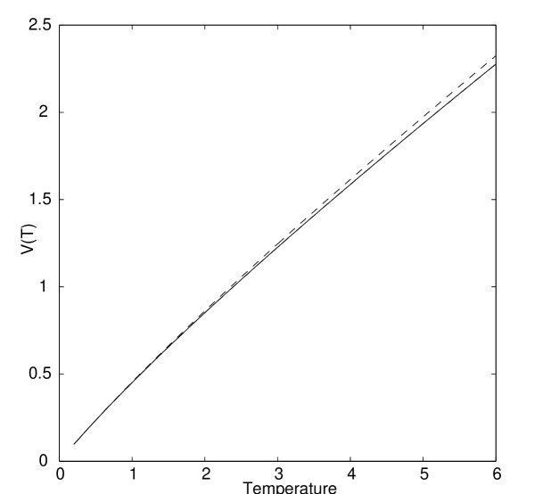
Figure 2: Potential energy versus temperature for $\beta=0.1$, the dashed line corresponds to the result obtained by Liv87 , while the solid line corresponds to equation 6.

For the last example, we consider a two dimensional system ($D=2$) exhibiting a second order phase transition, the so called dynamical lattice $\varphi^{4}$ model studied in Cai98 . This model is defined by the Hamiltonian

$$H=\sum_{i=1}^{N}\left(\frac{p_{i}^{2}}{2}-\frac{m^{2}}{2}q_{i}^{2}+\frac{\lambda}{4!}q_{i}^{4}\right)+\frac{J}{2}\sum_{\langle i,j\rangle}(q_{i}-q_{j})^{2}\>,$$ (7)

where $m$ and $\lambda$ are real parameters, $J=1$ is the coupling constant, and $\langle i,j\rangle$ denotes the summation over the close neighbors on a square lattice. In contrast with the other cases, where the $k=0$ mode $\alpha_{0}$ was a free parameter, in this example it is relevant and corresponds to the average of $q$ which is proportional to the magnetization of the system and is independent of time at equilibrium. The computation of the averaged potential energy is very similar to the $\beta$-FPU case:

$$v = \frac{1}{4}\sum_{k}\left(\omega_{0k}^{2}-m^{2}+\frac{\lambda}{2}\alpha_{0}^{2}\right)\alpha_{k}^{2}+\frac{\lambda}{32}\sum_{k\neq k^{\prime}}\alpha_{k}^{2}\alpha_{k^{\prime}}^{2}\>$$ (8)

$$+\frac{\lambda}{64}\sum_{k}\alpha_{k}^{4}-\frac{m^{2}}{2}\alpha_{0}^{2}+\frac{\lambda}{4!}\alpha_{0}^{4}\>.$$

The thermodynamic motion equations are

$$0 = \alpha_{0}\left(\frac{\lambda}{6}\alpha^{2}_{0}+\frac{\lambda}{4}Q-m^{2}\right)$$ (9)

$$\ddot{\alpha}_{k} = -\left(\omega^{2}_{0k}-m^{2}+\frac{\lambda}{2}\alpha^{2}_{0}+\frac{\lambda}{4}Q\right)\alpha_{k}+\frac{\lambda}{8}\alpha^{3}_{k}\>,$$ (10)

where $\omega_{0k}^{2}=4(\sin^{2}k_{x}/2+\sin^{2}k_{y}/2)$ is the free harmonic frequency ($k=(k_{x},k_{y})$ is now a vector in the plane), and $Q=\sum\alpha_{k}^{2}$ is an intensive variable.

Equation (9) has multiple solutions in $\alpha_{0}$ depending on the temperature through $Q=Q(T)$. Since $\alpha_{0}=\langle q_{i}\rangle$ is the order parameter, we anticipate the existence of a phase transition in the thermodynamic state. Indeed, the only solution is $\alpha_{0}=0$ for $Q>Q_{*}=4m^{2}/\lambda$ but for $Q<Q_{*}$ other solutions with finite values of the order parameter exist:

$$\alpha_{0}^{2}=\frac{6m^{2}}{\lambda}-\frac{3}{2}Q=\frac{3}{2}(Q_{*}-Q)\>.$$ (11)

To solve (10), we neglect the $\alpha_{k}^{3}$ term, as we did for the $\beta$-FPU case (large system limit) and obtain a wave equation with the dispersion relation: $\omega_{k}^{2}=\omega_{0k}^{2}+\Omega^{2}(T)$. $\Omega(T)$ is given by,

$$\Omega^{2} = \frac{\lambda}{2}(Q_{*}-Q),\quad Q<Q_{*}$$ (12)

$$\Omega^{2} = \frac{\lambda}{4}(Q-Q_{*}),\quad Q>Q_{*}\>.$$ (13)

where we used the definition of $Q_{*}$ and Eq. (11). We notice that $\Omega$ is the frequency corresponding to the absent $k=0$ mode.

Given the Jeans condition: $\alpha_{k}^{2}=2T/(N\omega_{k}^{2})$ we notice that as long as $\Omega\neq 0$ ($Q\neq Q_{*}$) the $\alpha_{k}^{3}$ term is a posteriori negligible, we can therefore expect results obtained with this approximation to be accurate everywhere but at (near) the transition. Another consequence of this condition is that most of the modes have comparable amplitudes for $\Omega\neq 0$, which then implies a Gaussian-like distribution for $q$. At the same order of approximation, in the thermodynamic limit, we can compute $Q(T)$, identifying it to a Riemann integral. Using the $\alpha_{k}$ given by the Jeans spectrum we obtain the following implicit equation for $Q(T)$,

$$Q(T)=\frac{T}{\pi}aK(a),\quad a=\frac{4}{4+\Omega^{2}(T)}\>,$$ (14)

where $K(a)$ is the complete elliptic integral of the first kind $\int^{\pi/2}_{0}d\theta/\sqrt{1-a^{2}\sin^{2}\theta}$.

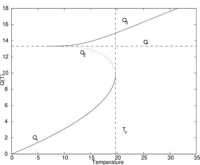
Figure 3: Solutions of the implicit equation (14), for $m^{2}=2$ and $\lambda=0.6$. We notice that depending on the value of $T$ up to three different solutions for $Q$ exists giving rise to three different branches respectively labelled $Q_{1}$, $Q_{2}$, $Q_{3}$. The critical temperature $T_{c}$ is identified.

The solutions of (14) has three branches, plotted on Fig. 3. We choose the same values $m^{2}=2$ and $\lambda=0.6$ as the ones used in Cai98 . We first notice the existence of a special temperature close to $19.69$ localizes the phase transition temperature. Two branches are below $Q_{*}=40/3$, and result from the expression (12) used in the implicit equation, the third one (on the top of the figure) corresponds to the expression (13). The fact that the wave form solutions are not valid for $Q=Q_{*}$ translate in the divergence of $K(a)$, since as $Q\rightarrow Q_{*}$, $a\rightarrow 1$. The divergence is logarithmic, and then for sufficiently small $T$, a solution around $Q_{*}$ of (14) always exists; resulting in the two upper branches being asymptotic to the $Q(T)=Q_{*}$ curve as $T$ goes to $0$.

In order to select one branch from another we compute their respective density of energy. According to equations (8) and (9), we have two different expressions for the density of energy,

$$e(T)=\left\{\begin{array}[]{ll}T-\frac{3m^{4}}{2\lambda}+\frac{3\lambda}{32}Q^{2}&,\quad Q<Q_{c}\\ T-\frac{\lambda}{32}Q^{2}&,\quad Q>Q_{c}\end{array}\right..$$ (15)

The results are plotted as the temperature versus the density of energy in Fig. 4 in analogy to the results presented in Cai98 . The physical relevant solution is the one whose energy is the smaller for a given temperature, which translate in the upper line in the figure. The transition is then identified at a density of energy $e_{c}=25.07$, whose corresponding temperature is $T_{c}=19.69$. These results are in good agreement with the one predicted by numerical simulations Cai98 : respectively $T_{c}=17.65$ and $e_{c}=21.1$. Using equation (11), we have also access to the square of the magnetization and there is also a good quantitative agreement with the numerical results. The discontinuous behavior of the magnetization at the transition is although surprising. This behavior was also observed numerically in Cai98 , and is explained by noticing that the true order parameter is $\langle|q|\rangle$ and not $|\langle q\rangle|$. In the present case, we can also wonder whether this behavior is due to the $N\rightarrow\infty$ limit taken before the $t\rightarrow\infty$. Indeed the neglected terms are relevant at the transition, and only become negligible around the transition after the $N\rightarrow\infty$ limit, which may affect the nature of the observed transition. However this behavior may also find its origin in the choice of writing the momentum as a superposition of $N^{\prime}$ random phased waves (motivated by the solutions of the linearized equations of motion) equal to the number of degrees of freedom $N$. Writing the momentum with the number of modes $N^{\prime}$ being a growing unbounded function of $N$ is sufficient to obtain a Gaussian process. Another representation may then be appropriate to tackle the transition region and for instance in Leo98 a high temperature approach was used to compute the critical temperature.

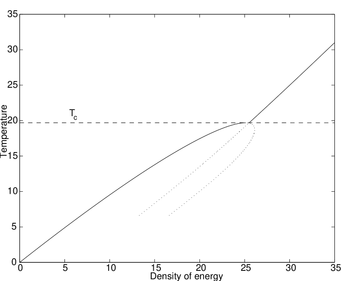
Figure 4: Temperature versus density of energy for $m^{2}=2$ and $\lambda=0.6$. The three different branches resulting from the solutions of $Q$ presented in Fig. 3 are represented. The physical line is the upper one. The transition is clearly identified with $T_{c}\approx 19.64$ and $\epsilon_{c}\approx 25.07$.

To conclude we point out that the thermodynamic motion equations method allowed us to compute the macroscopic properties of coupled nonlinear oscillator systems in one and two dimensions. Quantitative agreement with exact or numerical results of these quantities is obtained. Moreover the phase transition for the $\varphi^{4}$ model is detected and a good estimate of the critical energy and temperature are given even though we approximatively solved the thermodynamic motion equations. We expect that this method will be successful for other systems and speculate that the actual solving of the exact thermodynamics motion equation should lead to an exact thermodynamic limit. We believe it may also be possible to extend the scope of the method to systems out of equilibrium and describe their macroscopic evolution with the thermodynamic motion equations.