Large-N solutions of the Heisenberg and Hubbard-Heisenberg models on the anisotropic triangular lattice: application to Cs₂CuCl₄ and to the layered organic superconductors $\kappa$-(BEDT-TTF)₂X

Abstract

We solve the Sp(N) Heisenberg and SU(N) Hubbard-Heisenberg models on the anisotropic triangular lattice in the large-N limit. These two models may describe respectively the magnetic and electronic properties of the family of layered organic materials $\kappa$-(BEDT-TTF)₂X. The Heisenberg model is also relevant to the frustrated antiferromagnet, Cs₂CuCl₄. We find rich phase diagrams for each model. The Sp(N) antiferromagnet is shown to have five different phases as a function of the size of the spin and the degree of anisotropy of the triangular lattice. The effects of fluctuations at finite-N are also discussed. For parameters relevant to Cs₂CuCl₄ the ground state either exhibits incommensurate spin order, or is in a quantum disordered phase with deconfined spin-1/2 excitations and topological order. The SU(N) Hubbard-Heisenberg model exhibits an insulating dimer phase, an insulating box phase, a semi-metallic staggered flux phase (SFP), and a metallic uniform phase. The uniform and SFP phases exhibit a pseudogap. A metal-insulator transition occurs at intermediate values of the interaction strength.

I Introduction

The family of layered organic superconductors $\kappa$-(BEDT-TTF)₂X has attracted much experimental and theoretical interest[1, 2]. There are many similarities to the high-$T_{c}$ cuprates, including unconventional metallic properties and competition between antiferromagnetism and superconductivity[3]. The materials have a rich phase diagram as a function of pressure and temperature. At low pressures and temperatures there is an insulating antiferromagnetic ordered phase; as the temperature is increased a transition occurs to an insulating paramagnetic state. A first-order metal-insulator transition separates the paramagnetic insulating phase from a metallic phase; it is induced by increasing the pressure[4, 5]. The metallic phase exhibits various temperature dependences which are different from that of conventional metals. For example, measurements of the magnetic susceptibility and NMR Knight shift are consistent with a weak pseudogap in the density of states[6, 7].

The main purpose of this paper is to attempt to describe the magnetic ordering, the metal-insulator transition, and the unconventional metallic properties of these materials with two simplified models. We model the magnetic ordering in the insulating phase with the quantum Heisenberg antiferromagnet (HAF). We model the metallic phase as well as the metal-insulator transition with a hybrid Hubbard-Heisenberg model. To substitute for the lack of a small expansion parameter in either model, we enlarge the symmetry group from the physical SU(2) $\cong$ Sp(1) spin symmetry to Sp(N) (symplectic group) for the Heisenberg model[8, 9] and to SU(N) for the Hubbard-Heisenberg model[10, 11]. We then solve these models in the large-N limit and treat $1/N$ as our systematic expansion parameter. In section II we briefly summarize the physical SU(2) Heisenberg and Hubbard-Heisenberg model on the anisotropic triangular lattice. In section III we review the large-N theory of the Sp(N) quantum Heisenberg model. Based on the large-N solution of this model, we present the magnetic phase diagram in the parameter space of quantum fluctuation $n_{b}/N$ (where $n_{b}$ is the number of bosons in the Schwinger boson representation of the spin) and the magnetic frustration $J_{2}/J_{1}$. We discuss the effects of finite-N fluctuations on the Sp(N) magnetic phases with short-range order (SRO). We also discuss how our results are relevant to understanding recent neutron scattering experiments on Cs₂CuCl₄. In section IV we review the large-N theory of the SU(N) Hubbard-Heisenberg model. We present the phase diagram based on the large-N solution in the parameter space of the dimensionless ratio of the nearest-neighbor exchange to the hopping constant $J_{1}/t_{1}$ and the dimensionless anisotropy ratio $J_{2}/(J_{1}+J_{2})$. Away from the two nested limits $J_{1}=0$ and $J_{2}=0$ we find a metal-insulator transition which occurs at finite critical value of $J_{1}/t_{1}$. We also find that the density of states in the metallic state is suppressed at low temperatures, in qualitative agreement with the unconventional metallic properties seen in experiments. We conclude in section V with a brief review our results.

II Heisenberg and Hubbard-Heisenberg Models on the Anisotropic Triangular Lattice

Based on a wide range of experimental results and quantum chemistry calculations of the Coulomb repulsion between two electrons on the BEDT-TTF molecules it was argued in reference [3] that the $\kappa$-(BEDT-TTF)₂X family are strongly correlated electron systems which can be described by a half-filled Hubbard model on the anisotropic triangular lattice. The Hubbard Hamiltonian is:

$$H = -t_{1}\sum_{<{\bf{ij}}>}[c^{\dagger\sigma}_{\bf{i}}c_{{\bf{j}}\sigma}+H.c.]-t_{2}\sum_{<<{\bf{ij}}>>}[c^{\dagger\sigma}_{\bf{i}}c_{{\bf{j}}\sigma}+H.c.]$$ (1)

$$+ \frac{U}{2}\sum_{\bf{i}}(c^{\dagger\sigma}_{\bf{i}}c_{{\bf{i}}\sigma}-1)^{2}.$$ (2)

Here $c_{{\bf{i}}\sigma}$ is the electron destruction operator on site ${\bf{i}}$ and there is an implicit sum over pairs of raised and lowered spin indices $\sigma=\uparrow,\downarrow$. Matrix element $t_{1}$ is the nearest-neighbor hopping amplitude, and $t_{2}$ is the next-nearest-neighbor hopping along only one of the two diagonals of the square lattice as shown in figure 1. The sum $<{\bf{ij}}>$ runs over pairs of nearest-neighbor sites and $<<{\bf{ij}}>>$ runs for next-nearest-neighbors.

FIG. 1.: The anisotropic triangular lattice with two types of bonds. Note that this can also be viewed as a square lattice with an additional next-nearest neighbor interaction along only one of the two diagonals.

Physical insight can be attained by considering the Hubbard model for different values of the ratio $U/t$. In the limit of large $U/t$ the Hubbard model at half-filling is insulating and the spin degrees of freedom are described by a spin-1/2 Heisenberg antiferromagnet[12]:

$$H = J_{1}\sum_{<{\bf{ij}}>}\vec{S}_{\bf{i}}\cdot\vec{S}_{\bf{j}}+J_{2}\sum_{<<{\bf{ij}}>>}\vec{S}_{\bf{i}}\cdot\vec{S}_{\bf{j}},$$ (3)

where $\vec{S}_{\bf{i}}$ is the spin operator on site $\bf{i}$, and the exchange couplings $J_{1}=4t_{1}^{2}/U$ and $J_{2}=4t_{2}^{2}/U$. Competition between $J_{1}$ and $J_{2}$ leads to magnetic frustration. Using parameters from quantum chemistry calculations[13, 14, 15] it was estimated in reference [3] that $J_{2}/J_{1}\sim 0.3$ to $1$ for the $\kappa$-(BEDT-TTF)₂X family. Hence, magnetic frustration is important. The frustrated Heisenberg Hamiltonian interpolates between the square-lattice ($J_{2}=0$) and the linear chain ($J_{1}=0$). Much is known about these two limiting cases. Additional insight[16, 17] comes by considering different values of the ratio $J_{2}/J_{1}$. At $J_{2}=0$, the square lattice limit, there is long-range Néel order with a magnetic moment of approximately $0.6\mu_{B}$; see reference [12]. If $J_{2}$ is small but nonzero, the magnetic moment will be reduced by magnetic frustration. At $J_{2}/J_{1}$ around $0.5$, quantum fluctuations combined with frustration should destroy the Néel ordered state. As $J_{2}/J_{1}$ is further increased, the system may exhibit spiral long range order[17]. At $J_{1}=J_{2}$, the lattice is equivalent to the isotropic triangular lattice. Anderson suggested in 1973 that the ground state could be a spin liquid without long range order[18]. However, subsequent numerical work indicated that there is long-range-order with ordering vector $\vec{q}=(2\pi/3,2\pi/3)$[19]. Finally, at $J_{1}=0$ the model reduces to decoupled Heisenberg spin-1/2 chains which cannot sustain long range spin order[12] as per the quantum Mermin-Wagner theorem. For $J_{1}$ small but non-zero, the system consists of spin-1/2 chains weakly coupled in a zigzag fashion. The case of two such weakly coupled zigzag spin chains was studied by Okamoto and Nomura[20] and by White and Affleck[21] who showed that there is a spin gap in the spectrum $\Delta\sim e^{-{\rm const}\times J_{2}/J_{1}}$, and the ground state exhibits dimerization and incommensurate spiral correlations. Although our system consists of an infinite number of weakly coupled spin chains instead of two chains, we find similar behavior.

As $U/t$ decreases, charge fluctuations from electron hopping become significant. Competition between hopping and Coulomb repulsion leads to a transition from the insulator to a metal. We use the hybrid Hubbard-Heisenberg Hamiltonian[10, 11] with independent parameters $t$, $J$, and $U$ (where in general $J\neq 4t^{2}/U$) to describe some aspects of the transition:

$$H = \sum_{<{\bf{ij}}>}[-t_{1}(c^{\dagger\sigma}_{\bf{i}}c_{{\bf{j}}\sigma}+H.c.)+J_{1}(\vec{S}_{\bf{i}}\cdot\vec{S}_{\bf{j}}-\frac{1}{4}n_{\bf i}n_{\bf j})]$$ (4)

$$+ \sum_{<<{\bf{ij}}>>}[-t_{2}(c^{\dagger\sigma}_{\bf{i}}c_{{\bf{j}}\sigma}+H.c.)+J_{2}(\vec{S}_{\bf{i}}\cdot\vec{S}_{\bf{j}}-\frac{1}{4}n_{\bf i}n_{\bf j})]$$ (5)

$$+ \frac{U}{2}\sum_{\bf{i}}(c^{\dagger\sigma}_{\bf{i}}c_{{\bf{i}}\sigma}-1)^{2}\ .$$ (6)

Here $n_{\bf i}\equiv c_{\bf i}^{\dagger\sigma}c_{\bf{i}\sigma}$ is the number of fermions at site $\bf{i}$. The Hamiltonian reduces to the Hubbard model when $J_{1}=J_{2}=0$ and the Heisenberg model for $t_{1},t_{2}\to 0$. In the square lattice limit and at half-filling, perfect nesting drives the system to an antiferromagnetic insulator at arbitrarily small value of the interactions. As diagonal hopping $t_{2}$ is turned on, however, nesting of the Fermi surface is no longer perfect and the metal-insulator transition (MIT) occurs at non-zero critical interaction strength.

III Sp(N) Heisenberg Model

We first focus on the spin degree of freedom, appropriate to the insulating phase of the layered organic materials, by solving the Heisenberg model in a large-N limit. Our choice of the large-N generalization of the physical SU(2) spin-$1/2$ problem is dictated by the desire to find an exactly solvable model which has both long-range ordered (LRO) and short-range ordered (SRO) phases. This leads us to symmetric (bosonic) SU(N) or Sp(N) generalizations. The former can only be applied to bipartite lattices. The latter approach has been applied to the antiferromagnetic Heisenberg model on the square lattice with first-, second-, and third-neighbor coupling (the $J_{1}-J_{2}-J_{3}$ model)[8], the isotropic triangular lattice[22], and the kagomé lattice[22]. As the anisotropic triangular lattice is not bipartite, we must choose the Sp(N) generalization[8].

A Brief Review of the Approach

To ascertain the likely phase diagram of the frustrated Heisenberg antiferromagnet, we consider the Sp(N) symplectic group generalization of the physical SU(2)$\cong$ Sp(1) antiferromagnet[8, 22]. The model can be exactly solved in the $N\rightarrow\infty$ limit. Both LRO and SRO can arise if we use the symmetric (bosonic) representations of Sp(N). We begin with the bosonic description of the SU(2) HAF, where it can be shown that apart from an additive constant, the Hamiltonian may be written in terms of spin singlet bond operators:

$$H=-\frac{1}{2}\sum_{\bf{ij}}J_{\bf{ij}}(\varepsilon_{\alpha\beta}b_{\bf{i}}^{\dagger\alpha}b_{\bf{j}}^{\dagger\beta})(\varepsilon^{\gamma\delta}b_{\bf{i}\gamma}b_{\bf{j}\delta})$$ (7)

where we have used the bosonic representation for spin operator

$$\vec{S}_{\bf i}=\frac{1}{2}b_{\bf i}^{\dagger\alpha}\vec{\sigma}_{\alpha}^{\beta}b_{{\bf i}\beta}\ ,$$ (8)

where $\alpha=\uparrow,\downarrow$ labels the two possible spins of each boson. The antisymmetric tensor, $\varepsilon_{\alpha\beta}$ is as usual defined to be:

$$\varepsilon=\left(\begin{array}[]{cc}0&1\\ -1&0\end{array}\right)\ .$$ (11)

We enforce the constraint $n_{b}=b_{\bf{i}}^{\dagger\alpha}b_{\bf{i}\alpha}=2S$ to fix the number of bosons, and hence the total spin, on each site. The SU(2) spin singlet bond creation operator $\varepsilon_{\alpha\beta}b_{\bf{i}}^{\dagger\alpha}b_{\bf{j}}^{\dagger\beta}$ may now be generalized to the Sp(N)-invariant form ${\mathcal{J}}_{\alpha\beta}b_{\bf{i}}^{\dagger\alpha}b_{\bf{j}}^{\dagger\beta}$. Global Sp(N) rotations may be implemented with $2N\times 2N$ unitary matrices $U$:

$$b \to Ub$$ (12)

$$U^{\dagger}{\mathcal{J}}U = {\mathcal{J}}.$$ (13)

Here

$${\mathcal{J}}=\left(\begin{array}[]{cccccc}&1&&&&\\ -1&&&&&\\ &&&1&&\\ &&-1&&&\\ &&&&\ddots&\\ &&&&&\ddots\end{array}\right)$$ (14)

generalizes the $\epsilon$ tensor to $N>1$, and $b_{\bf{i}\alpha}$ with $\alpha=1\ldots 2N$ is the Sp(N) boson destruction operator. The Hamiltonian of the Sp(N) HAF may then be written:

$$H=-\sum_{\bf{ij}}\frac{J_{\bf{ij}}}{2N}\left({\mathcal{J}}_{\alpha\beta}b_{\bf{i}}^{\dagger\alpha}b_{\bf{j}}^{\dagger\beta}\right)\left({\mathcal{J}}^{\gamma\delta}b_{\bf{i}\gamma}b_{\bf{j}\delta}\right)$$ (15)

where again the Greek indices run over $1\ldots 2N$, and the constraint $b_{\bf{i}}^{\dagger\alpha}b_{\bf{i}\alpha}=n_{b}$ is imposed at every site of the lattice. We have rescaled $J_{\bf{ij}}/2\rightarrow J_{\bf{ij}}/2N$ to make the Hamiltonian of $O(N)$. For fixed $J_{1}/J_{2}$ we have a two-parameter ($n_{b}$, $N$) family of models with the ratio $\kappa\equiv n_{b}/N$ determining the strength of the quantum fluctuations. In the physical Sp(1) limit, $\kappa=1$ corresponds to spin-1/2. At large $\kappa$ (equivalent to the large-spin limit of the physical SU(2) model) quantum effects are small and the ground states break global Sp(N) spin-rotational symmetry. LRO then corresponds to Bose condensation which we quantify by defining

$$b_{\bf{i}m\sigma}\equiv\left(\begin{array}[]{c}\sqrt{N}x_{{\bf i}\sigma}\\ \tilde{b}_{{\bf i}\tilde{m}\sigma}\end{array}\right)\ .$$ (16)

Here the spin-quantization axis has been fixed by introducing the paired-index notation $\alpha\equiv(m,\sigma)$ with $m=1\ldots N$, $\sigma=\uparrow,\downarrow$, and $\tilde{m}=2\ldots N$. The c-number spinors $x_{\sigma}$, when non-zero, quantify the Bose condensate fraction, and are given by $\langle b_{{\bf i}m\sigma}\rangle=\sqrt{N}\delta^{1}_{m}x_{\bf{i}\sigma}$. For sufficiently small $\kappa$, however, quantum fluctuations overwhelm the tendency to order and there can be only magnetic SRO.

Upon inserting equation 16 into equation 15, decoupling the quartic boson terms within the corresponding functional integral by introducing complex-valued Hubbard-Stratonovich fields $Q_{\bf{ij}}$ directed along the lattice links, enforcing the constraint on the number of bosons on each site with Lagrange multipliers $\lambda_{\bf{i}}$, and finally integrating out the $b$-fields, we obtain an effective action proportional to $N$. Thus, as $N\to\infty$, the effective action may be replaced by its saddle-point value. At the saddle-point, the $Q_{\bf{ij}}$, $\lambda_{\bf{i}}$, and $x_{\bf{i}\sigma}$ fields are expected to be time-independent, so the effective action can be put into correspondence with a suitable mean-field Hamiltonian. The Hamiltonian may be diagonalized by a Bogoliubov transformation, yielding a total ground state energy $E_{MF}$ given by[22]

$$\frac{E_{MF}[Q,\lambda]}{N} = \sum_{\bf{i>j}}\left(\frac{J_{\bf{ij}}}{2}{|Q_{\bf{ij}}|}^{2}-\frac{J_{\bf{ij}}}{2}Q_{\bf{ij}}\varepsilon^{\sigma\sigma^{\prime}}x_{\bf{i}\sigma}x_{\bf{j}\sigma^{\prime}}+H.c.\right)$$ (17)

$$- \sum_{\bf{i}}\lambda_{\bf{i}}\left(1+\frac{n_{b}}{N}-|x_{\bf{i}\sigma}|^{2}\right)+\sum_{\bf k}\omega_{\bf k}$$ (18)

where $\omega_{\bf k}$ are eigenenergies obtained from diagonalizing the mean-field Hamiltonian. Finding the ground state of the Sp(N) HAF now reduces to the problem of minimizing $E_{MF}$ with respect to the variables $Q_{{\bf{ij}}}$ and $x_{\bf{i}\sigma}$, subject to the Lagrange-multiplier constraints

$$\frac{\partial E_{MF}[Q,\lambda]}{\partial\lambda_{\bf i}}=0\ .$$ (19)

It is essential to note that the action possesses local U(1) gauge symmetry under local phase rotations by angle $\theta_{i}(\tau)$:

$$b_{{\bf i}\alpha}\to b_{{\bf i}\alpha}~{}e^{-i\theta_{\bf{i}}(\tau)}$$ (20)

$$Q_{\bf{ij}}\to Q_{\bf{ij}}~{}e^{i\theta_{\bf{i}}(\tau)+i\theta_{\bf{j}}(\tau)}$$ (21)

$$\lambda_{\bf{i}}\to\lambda_{\bf{i}}+\frac{\partial\theta_{\bf{i}}}{\partial\tau}\ .$$ (22)

This symmetry reminds us that the representation of spin operators in terms of the underlying bosons is redundant as the phase of each boson fields can be shifted by an arbitrary amount without affecting the spin degree of freedom. Two gauge invariant quantities of particular importance for our classification of the phases are $|Q_{\bf{ij}}|$, and $\sum_{\bf{i}}\lambda_{\bf i}$.

Extrema of $E_{MF}$ are found numerically with the simplex-annealing method[23]. We work with a lattice of $40\times 40$ sites and check that this is sufficiently large to accurately represent the thermodynamic limit. Constraint equation 19 is tricky, however, as $E_{MF}[\lambda_{\bf i}]$ is neither a minimum, nor a maximum with respect to the $\lambda_{\bf i}$ directions at the saddle point. The problem is solved by decomposing $\lambda_{\bf{i}}$ into its mean value $\bar{\lambda}$ and the deviations from the mean, $\delta\lambda_{\bf i}\equiv\lambda_{\bf i}-\bar{\lambda}$. As $\bar{\lambda}$ is gauge-invariant, we solve the constraint equation 19 separately for it by applying Newton’s method. The resulting $E_{MF}[\bar{\lambda},\delta\lambda_{\bf i}]$ can then be maximized in the remaining $\delta\lambda_{\bf i}$ directions. Individual values of $\delta\lambda_{\bf{i}}$ are in general non-zero, but by definition it must be the case that $\sum_{\bf i}\delta\lambda_{\bf{i}}=0$.

B Phase Diagram of the Sp(N) Heisenberg antiferromagnet

To make progress in actually solving the model, we now make the assumption that spontaneous symmetry breaking, if it occurs, does not lead to a unit cell larger than 4 sites. Our choice of unit cell is shown in figure 2.

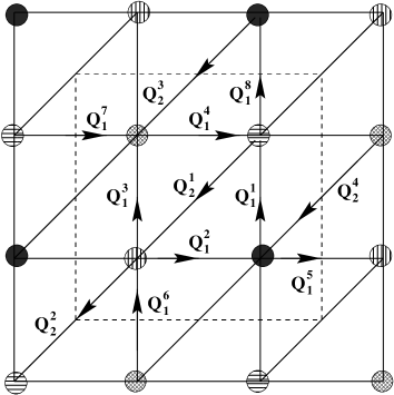
FIG. 2.: The $2\times 2$-site unit cell for the Sp(N) Heisenberg antiferromagnet on the anisotropic triangular lattice. The complex-valued, directed, $Q_{1}^{1}$ to $Q_{1}^{8}$ fields live on the links of the square lattice, while $Q_{2}^{1}$ to $Q_{2}^{4}$ live on the diagonal links. Arrows denote the orientation of the $Q_{\bf ij}$ fields.

The $2\times 2$ unit cell requires 12 different complex-valued Q-fields (8 on the square links, and 4 along the diagonal links) and 4 different $\lambda$ fields and $x$ spinors at each of the four sites. However, we have checked that at every saddle-point in the SRO region of the phase diagram ($x_{{\bf i}\sigma}=0$) each of the 8 Q-fields on the horizontal and vertical links take the same value. Likewise, the 4 Q-fields on the diagonals are all equal, as well as all 4 $\lambda$-fields. Thus the $2\times 2$-site unit cell can be reduced to only a single site per unit cell as shown in figure 3. We expect this to also hold in the LRO phases, in accord with previous work on the Sp(N) model[22].

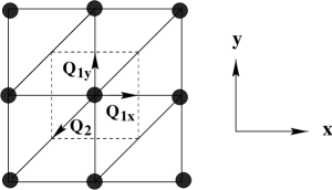
FIG. 3.: The one-site unit cell for the Sp(N) Heisenberg antiferromagnet on the anisotropic triangular lattice.

The zero-temperature phase diagram is a function of two variables: $J_{2}/J_{1}$ and $\kappa$. The various saddle points can be classified in several ways. Both SRO and LRO phases may be characterized in terms of an ordering wavevector $\vec{q}$ via the relation $\vec{q}=2\vec{k}_{min}$, where $\vec{k}_{min}$ is the wavevector at which the bosonic spinon energy spectrum has a minimum. The spin structure factor $S(\bf{q})$ peaks at this wavevector[22]. LRO is signaled by non-zero spin condensate $x_{\bf{i}\sigma}$, which we assume occurs at only one wavevector, $\vec{k}_{min}$; that is, $x_{\bf{j}\uparrow}=x\exp(i\vec{k}_{min}\cdot\vec{r}_{\bf j})$ and $x_{\bf{j}\downarrow}=-ix\exp(-i\vec{k}_{min}\cdot\vec{r}_{\bf j})$. The phases may be further classified[8] according to the particular value of $\vec{q}$. There can be commensurate collinear ordering tendencies where the spins rotate with a period that is commensurate with the underlining lattice. Alternatively, there may be incommensurate coplanar ordering tendencies where the spins rotate in a two dimensional spin space with a period that is not commensurate with the lattice.

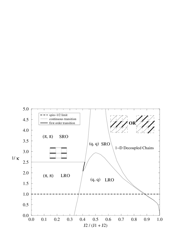
FIG. 4.: Zero-temperature phase diagram of the Sp(N) Heisenberg antiferromagnet at large-N. The strength of the quantum fluctuations is set by the parameter $1/\kappa$ (vertical axis). Dimerization patterns induced by finite-N fluctuations are shown in the insets.

The phase diagram is shown in figure 4. Note that the general shape of the phase diagram is qualitatively consistent with the finding of spin wave calculations[17, 16] that quantum fluctuations are largest for $J_{2}/J_{1}\sim 0.5$ and large $J_{2}/J_{1}$. For large enough values of $\kappa$, the ground state has magnetic LRO. As the magnetic LRO phases break Sp(N) symmetry, there are gapless Goldstone spin-wave modes. As a check on the calculation, we note that in the $\kappa\rightarrow\infty$ limit there is a transition between the Néel ordered and incommensurate $(q,q)$ LRO phase at $J_{2}/J_{1}=0.5$ in agreement with the classical large-spin limit. At smaller values of $\kappa$ there are quantum disordered phases that preserve global Sp(N) symmetry. In the $N\rightarrow\infty$ limit these are rather featureless spin liquids with gapped, free, spin-1/2 bosonic excitations (spinons). Finite-N fluctuations, however, induce qualitative changes to the commensurate SRO phases (see below). In the limiting case of the nearest-neighbor square lattice, $J_{2}=0$, we reproduce the previously obtained result[8] that Néel order arises for $\kappa>0.4$. In the opposite limit of decoupled one dimensional spin chains, $J_{1}=0$, the ground state is in a disordered phase at all values of $\kappa$. There are five phases in all, three commensurate and two incommensurate, as detailed in the following two subsections.

1 Commensurate phases

At small to moderate $J_{2}/J_{1}$ there are two phases with $Q_{1x}=Q_{1y}\neq 0$, and $Q_{2}=0.$ The eigenspectrum $\omega_{\bf k}$ has its minimum at ${\bf k}=\pm(\pi/2,\pi/2)$, with the implication that the spin-spin correlation function peaks at $\vec{q}=(\pi,\pi)$. Néel LRO with $x_{\bf{i}\sigma}\neq 0$ appears when $\kappa$ is sufficiently large. The boundary between LRO and SRO phases is independent of $J_{2}/J_{1}$ except at one end of the boundary, but this is expected to be an artifact of the large-N limit[22]. Finite-N corrections should bend this horizontal phase boundary.

At large $J_{2}/J_{1}$ and small $\kappa$ the ground state is a disordered state characterized by $Q_{1x}=Q_{1y}=0$ and $Q_{2}\neq 0$. The chains decouple from one another exactly in the large-N limit, but at any finite-N the chains will be coupled by the fluctuations about the saddle point. Also, $x_{\bf{i}\sigma}=0$ as it must, by the Mermin-Wagner theorem. The Sp(N) solution does not properly describe the physics of completely decoupled spin-$1/2$ chains. All spin excitations are gapped, and there is dimerization at finite-N (see below). This behavior is in marked contrast to the gapless, undimerized ground state of the physical SU(2) spin-$1/2$ nearest-neighbor Heisenberg chain[12].

2 Incommensurate phases

At intermediate values of $J_{2}/J_{1}$, there are two incommensurate phases with $Q_{1x}=Q_{1y}\neq 0$, and $Q_{2}\neq 0$. The ordering wavevector $\vec{q}=(q,q)$ with $q$ varying continuously from $\pi$ to $\pi/2$, a sign of helical spin order in a given plane. The inverse $\kappa_{c}^{-1}$ of the critical $\kappa$ separating LRO from SRO peaks near the isotropic triangular point $J_{2}/J_{1}=1$, where it agrees in value to that reported in a prior study of the triangular lattice[22], and then decreases with a long tail as $J_{2}/J_{1}$ increases. As the one-dimensional limit of decoupled chains is approached, ${\kappa}_{c}\rightarrow\infty$. Again this accords with the Mermin-Wagner theorem.

All the phase transitions are continuous except for the transitions between the $(\pi,\pi)$ LRO phase and the $(q,q)$ SRO phase which is first order. Fluctuations at finite-N, however, modify the mean-field results[8]. The modifications are only quantitative for the LRO phases, and for the incommensurate SRO phase. In particular, instantons in the U(1) gauge field have little effect in the incommensurate SRO phase which is characterized by non-zero $Q_{2}$. The $Q_{2}$ fields carry charge $\pm 2$, so when they acquire a non-zero expectation value, this is equivalent to the condensation of a charge-2 Higgs field. Fradkin and Shenker[25] showed some time ago that a Higgs condensate in 2+1 dimensions quenches the confining U(1) gauge force. Singly-charged spinons are therefore deconfined, instead the instantons which carry magnetic flux are confined, and no dimerization is induced[8]. The relevant non-linear sigma model which describes the transition from an ordered incommensurate phase to a quantum disordered phase has been studied by Chubukov, Sachdev, and Senthil[26].

In the case of the commensurate $(\pi,\pi)$ SRO and the decoupled chain phases, instantons do alter the states qualitatively. The Berry’s phases associated with the instantons lead to columnar spin-Peierls order[24, 8] (equivalent to dimer order) as indicated in figure 4. The dimerization pattern induced in the decoupled chain phase is similar to that found by White and Affleck[21] for a pair of chains with zigzag coupling. Furthermore, spinon excitations are confined into pairs by the U(1) gauge force.

Note that the deconfined spinons in the $(q,q)$ SRO phase are qualitatively different than the spinons found in the limit of completely decoupled chains, $J_{1}=0$. The $(q,q)$ SRO phase exhibits true 2-dimensional fractionalization, in contrast to the decoupled one-dimensional chains. The spinons are massive, again in contrast to those found in one-dimensional half-odd-integer spin chains. The transition from the dimerized chain phase at small $J_{1}/J_{2}$, which has confined spinons, to the deconfined incommensurate phase at larger $J_{1}/J_{2}$ is described by a 2+1 dimensional Z₂ gauge theory[27]. In fact the $(q,q)$ SRO phase is similar to a resonating valence bond (RVB) state recently found on the isotropic triangular lattice quantum dimer model[28]. The phase has “topological” order; consequently when the lattice is placed on a torus (that is, when periodic boundary conditions are imposed), the ground state becomes four-fold degenerate in the thermodynamic limit[29, 30].

C Physical Spin-$1/2$ Limit

It is interesting to examine in more detail the physical spin-$1/2$ limit corresponding to $\kappa=1$. In figure 5 we plot the ordering wavevector $q$ as a function of the ratio $J_{2}/(J_{1}+J_{2})$. Note that quantum fluctuations cause (i) the Néel phase to be stable for larger values of $J_{2}/J_{1}$ than classically, and (ii) the wave vector associated with the incommensurate phases deviates from the classical value. Similar behavior was also found in studies based on a series expansion[31], and slave bosons including fluctuations about the saddle point[32].

FIG. 5.: Ordering wavevector $q$ (in units of $\pi/a$) of the large-N Sp(N) Heisenberg antiferromagnet at $\kappa=1$, which corresponds to spin-1/2 in the physical Sp(1) limit. The solid line is the classical ordering wavevector[17].

Commensurate $q=\pi$ Néel order persists up to $J_{2}/(J_{1}+J_{2})=0.369$, and this is followed by the incommensurate LRO phase for $0.369<J_{2}/(J_{1}+J_{2})<0.880$. Then a tiny sliver of the incommensurate SRO phase arises for $0.880<J_{2}/(J_{1}+J_{2})<0.886$. Finally there is the decoupled chain phase for $0.886<J_{2}/(J_{1}+J_{2})\leq 1$. A strikingly similar phase diagram has been obtained by the series expansion method[31]. A comparison between the Sp(N) and series expansion results is shown in figure 6. Both methods suggest that there exists a narrow SRO region between Néel and incommensurate ordered phases, though in the Sp(N) case the region does not extend all the way up to $\kappa=1$. Possibly finite-$N$ corrections to this large-N result could change the phase diagram quantitatively such that the $(q,q)$ SRO phase persists up to $\kappa=1$ in agreement with the series expansion results. Another difference is that the Sp(N) result shows no dimerization in this narrow SRO region (due to the above-mentioned Higgs mechanism), while the series expansion indicates possible dimer order.

FIG. 6.: Comparison of Sp(N) phase diagram at $\kappa=1$ with the results of a series-expansion[31].

Similar results have also been obtained in a weak-coupling renormalization group (RG) treatment of the Hubbard model on the anisotropic triangular lattice[33]. For the special case of a pure square lattice (with next-nearest-neighbor hopping $t_{2}=0$) at half-filling, the antiferromagnetic (AF) couplings diverge much faster during the RG transformations than couplings in the BCS sector, indicating a tendency towards magnetic LRO. As $t_{2}$ is turned on, BCS and AF instabilities begin to compete. For sufficiently large $t_{2}$, a crossover occurs to a $d_{x^{2}-y^{2}}$ BCS instability, suggesting that the system is now in a magnetic SRO state. Further increasing $t_{2}$ to reach the isotropic triangular lattice ($t_{1}=t_{2}$) there are indications that long-range AF order re-enters. Finally, for $t_{2}\gg t_{1}$ LRO tendencies are again eliminated, this time by the strong one-dimensional fluctuations. It is remarkable that the same sequence of ordering and disordering tendencies – LRO to SRO to LRO to SRO – occurs in all three approximate solutions.

D Application To Materials

The region of the phase diagram intermediate between the square lattice and the isotropic triangular lattice is relevant to the insulating phase of the organic $\kappa$-(BEDT-TTF)₂X materials. The expected range in the spin exchange interaction[3] is $J_{2}/J_{1}\sim 0.3$ to $1$. Depending on the precise ratio $J_{2}/J_{1}$, our phase diagram indicates that these materials could be in the Néel ordered phase, the $(q,q)$ LRO phase, or possibly the paramagnetic $(q,q)$ SRO phase (see above). In fact antiferromagnetic ordering with a magnetic moment of $0.4$ to $1\times\mu_{B}$ per dimer has been seen in the splitting of proton NMR lines in the $\kappa$-(BEDT-TTF)₂Cu[N(CN)₂]Cl compound[35]. It is conceivable that a quantum phase transition from the Néel ordered phase to the paramagnetic $(q,q)$ SRO phase or to the $(q,q)$ LRO phase can be induced by changing the anion X.

Coldea et al.[34] have recently performed a comprehensive neutron scattering study of Cs₂CuCl₄. They suggest that this material is described by the spin-1/2 version of our model with $J_{2}/J_{1}=2.5$ and $J_{2}=0.37$ meV. The measured incommensurability with respect to Néel order, $\pi-q$, is reduced below the classical value by a factor $0.47$, consistent with series results[31] (our Sp(N) solution shows a smaller reduction). Maps of the excitation spectra show that the observed dispersion is renormalized upward in energy by a factor of $1.67$, which can be compared to theoretical values of $1.18$ for the square lattice and $1.57$ for decoupled chains. Furthermore, the dynamical structure factor $S(\vec{q},\omega)$ does not exhibit well defined peaks corresponding to well defined spin-1 magnon excitations. Instead there is a continuum of excitations similar to those expected and seen in completely decoupled spin-$1/2$ Heisenberg chains. In the case of a chain these excitations can be interpreted as deconfined gapless spin-1/2 spinons.

In the relevant parameter regime, $J_{2}/J_{1}$ = 2.5, the large-N Sp(N) phase diagram predicts that the ground state is spin-ordered with an incommensurate wavevector $(q,q)$. However, as noted above, finite-N corrections could move the phase boundaries so that the physical spin-1/2 limit is in fact described by the $(q,q)$ SRO phase. In this phase there is a non-zero gap to the lowest lying excitations [which occur at wave vector $(k_{min},k_{min})=(q/2,q/2)$] rather than gapless excitations. At $\kappa=0.56$ and $J_{2}/J_{1}=2.5$, in the large-N limit, the system is in the $(q,q)$ SRO phase of figure 4 and the spinon gap is approximately $0.05J_{2}$. This is much smaller than the resolution of the experiment [see Figure 2(a) in reference [34]], in which excitation energies have only been measured down to about 0.5 $J_{2}$. The corresponding spinon dispersion is shown in figure 7. Again we stress that the spinons in the incommensurate SRO phase are qualitatively different than those which arise in a one-dimensional chain.

FIG. 7.: Spinon dispersion along the $(1,1)$ direction in the deconfined $(q,q)$ SRO phase for $\kappa=0.56$, $J1=0.148$ meV, and $J2=0.37$ meV; thus, $J2/J1=2.5$. The lowest energy excitations occur at an incommensurate wavevector of $k\approx 0.26\times\pi$ where there is a non-zero energy gap of approximately $0.02$ meV.

In the deconfined $(q,q)$ SRO phase, there are no true spinwave excitations, as spin rotational symmetry is unbroken. Nevertheless, when the gap to create a spinon is small, the spinwave description remains useful. For example, in neutron scattering experiments, spinons are created in pairs, as each spinon carries spin-$1/2$. So a spinwave may be viewed as an excitation composed of two spinons, though of course this spinwave does not exhibit the sharp spectral features of a true Goldstone mode. At large-N the spinons do not interact; finite-N fluctuations will lead to corrections in the combined energy and to a finite lifetime. The minimum energy of such a spinwave of momentum $\vec{q}$ is given, in the large-N limit, by:

$$E_{\vec{q}}={\rm Min}\{\omega(\vec{q}/2+\vec{p}/2)+\omega(\vec{q}/2-\vec{p}/2)\}$$ (23)

where the minimization is with respect to all possible relative momenta $\vec{p}$. The resulting spinwave dispersion is plotted in figure 8 alongside the classical result, scaled to the same value of the spin. The Sp(N) calculation shows a rather large upward renormalization in the energy scale compared to the classical calculation; this is a result of the quantum fluctuations which are retained in the large-N limit.

FIG. 8.: Minimum energy of two spinons in the $(q,q)$ SRO phase (solid line) compared to that of classical spinwaves (dashed line) for the same parameters as in figure 7. The dispersion, in the case of the Sp(N) theory, is obtained from equation 23. The classical spinwave dispersion is obtained from reference [17] where it was scaled to spin-$1/2$. These energies have been multiplied here by a factor of $\kappa^{2}\approx 0.31$ to account for the reduced magnitude of the spin. The large upward renormalization in the Sp(N) excitation energies compared to the classical energies is due to quantum fluctuations.

In the incommensurate $(q,q)$ LRO phase ($\kappa=1$ and $N\rightarrow\infty$) the spinon spectrum has gapless excitations, as shown in figure 9. Apart from the absence of the small gap, the spinwave dispersion in the ordered phase is similar to the minimum energy spectrum in the disordered phase. Again there is an upward renormalization of the energy scale as shown in figure 10, though the ratio is relatively smaller than in the more quantum $\kappa=0.56$ case. The size of the renormalization is in good agreement with that seen in the Cs₂CuCl₄ experiment[34]. It is important to note that finite-N gauge fluctuations bind spinons in the LRO phase into true spinwave excitations, with corresponding sharp spectral features. In contrast, as noted above, spectral weight is smeared out in the SRO phase. A large spread of spectral weight is seen in the neutron scattering experiments[34]. But as the incommensurate SRO and LRO states are separated by a continuous phase transition (see figure 4), in the vicinity of the phase boundary it is difficult to distinguish the two types of excitation spectra. The spin moment in the LRO phase is small there, as is the gap in the SRO phase. Further experiments on Cs₂CuCl₄ may be needed to determine which of the two phases is actually realized in the material.

FIG. 9.: Spinon dispersion along the $(1,1)$ direction in the incommensurate $(q,q)$ LRO phase. As in figure 7, $J1=0.148$ meV and $J2=0.37$ meV, but now $\kappa=1$. Gapless excitations occur at an incommensurate wavevector of $k\approx 0.27\times\pi$.

FIG. 10.: The same as figure 8 except in the incommensurate $(q,q)$ LRO phase with the same parameters as in figure 9: $J1=0.148$ meV and $J2=0.37$ meV, and $\kappa=1$.

IV SU(N) Hubbard-Heisenberg Model

We now turn our attention to the charge degrees of freedom by studying the hybrid Hubbard-Heisenberg model. This model should provide a reasonable description of the layered organic materials because the Hubbard interaction is comparable in size to the hopping matrix elements, $U\approx t$. Thus the stringent no-double-occupancy constraint of the popular $t-J$ model should be relaxed. In the large-N limit it is also better to work with the hybrid Hubbard-Heisenberg model than with the pure Hubbard model because the crucial spin-exchange processes are retained in the large-N limit[11]. In the Hubbard model these are only of order $1/N$ and therefore vanish in the mean-field description.

As there are now both charge and spin degrees of freedom, it is no longer possible to employ purely bosonic variables, in contrast to the previous section. Instead we use antisymmetric representations of the group SU(N) as the large-N generalization of the physical SU(2) system. As shown below, this generalization precludes the possibility of describing magnetic LRO or superconducting phases, at least in the large-N limit. However, as the same representation is placed on each lattice site, this large-N generalization works equally well for bipartite and non-bipartite lattices. It has been applied to the spin-1/2 Heisenberg antiferromagnet on the kagomé lattice[36].

A Brief Review of the Approach

The Hubbard-Heisenberg Hamiltonian on the anisotropic triangular lattice is specified by equation 6. The generalized SU(N) version is obtained[11] by simply letting the spin index $\sigma$ in equation 6 run from 1 to N (where N is even):

$$H = \sum_{<{\bf{ij}}>}[-t_{1}(c^{\dagger\sigma}_{\bf{i}}c_{{\bf{j}}\sigma}+H.c.)-\frac{J_{1}}{N}(c^{\dagger\alpha}_{\bf{i}}c_{{\bf{j}}\alpha}c^{\dagger\beta}_{\bf{j}}c_{{\bf{i}}\beta}+\frac{1}{2}n_{\bf{i}}n_{\bf{j}})]$$ (24)

$$+ \sum_{<<{\bf{ij}}>>}[-t_{2}(c^{\dagger\sigma}_{\bf{i}}c_{{\bf{j}}\sigma}+H.c.)-\frac{J_{2}}{N}(c^{\dagger\alpha}_{\bf{i}}c_{{\bf{j}}\alpha}c^{\dagger\beta}_{\bf{j}}c_{{\bf{i}}\beta}+\frac{1}{2}n_{\bf{i}}n_{\bf{j}})]$$ (25)

$$+ \frac{U}{N}\sum_{\bf{i}}(c^{\dagger\sigma}_{\bf{i}}c_{{\bf{i}}\sigma}-N/2)^{2}\$$ (26)

where all spin indices are summed over. Here we have also rescaled the interaction strengths $J_{i}/2\rightarrow J_{i}/N$ and $U/2\rightarrow U/N$ to make each of the terms in the Hamiltonian of order N. At half-filling, the only case we consider here, a further simplification occurs as the term $J_{\bf{ij}}n_{\bf{i}}n_{\bf{j}}$ is simply a constant. There is no possibility of phase separation into hole-rich and hole-poor regions, nor can stripes form[37], as the system is at half-filling. We drop this constant term in the following analysis.

We could also include a biquadratic spin-spin interaction of the form $\tilde{J}(\vec{S}_{\bf i}\cdot\vec{S}_{\bf j})^{2}$ with $\tilde{J}>0$. In the physical SU(2) limit this term does nothing except renormalize the strength of the usual bilinear spin-spin interaction. But for $N>2$ it suppresses dimerization[11], as the concentration of singlet correlations on isolated bonds is particularly costly when the biquadratic term is included. Thus there exists a family of large-N theories parameterized by the dimensionless ratio $\tilde{J}/J$, each of which has the same physical SU(2) limit. In this paper, however, we set $\tilde{J}=0$ as we find that the phase most likely to describe the metallic regime of the organic superconductors is a uniform phase with no dimerization which is stable even at $\tilde{J}=0$.

After passing to the functional-integral formulation in terms of Grassman fields, the quartic interactions are decoupled by a Hubbard-Stratonovich transformation which introduces real-valued auxiliary fields $\phi$ on each site and complex-valued $\chi$ fields directed along each bond:

$$\phi_{\bf{i}}={\it i}\frac{U}{N}(c^{*\sigma}_{\bf{i}}c_{{\bf{i}}\sigma}-N/2),\quad\chi_{\bf{i}\bf{j}}=\frac{J_{\bf{i}\bf{j}}}{N}c^{*\sigma}_{\bf{i}}c_{{\bf{j}}\sigma}\ .$$ (27)

Clearly $\langle\phi_{\bf{i}}\rangle$ is proportional to the local charge density relative to half-filling (corresponding to $N/2$ fermions at each site) and $\chi_{\bf{i}\bf{j}}$ may be viewed as an effective hopping amplitude for the fermions between site $\bf{i}$ and $\bf{j}$. The effective action in terms of these auxiliary fields, which may be viewed as order parameters, can now be obtained by integrating out the fermions. We note that, unlike the bosonic formulation of the pure antiferromagnet, here there is no possibility of magnetic LRO as the order parameters $\chi$ and $\phi$ are global SU(N) invariants, and of course there is no possibility of Bose condensates in the fermionic antisymmetric representation of SU(N). Superconductivity likewise is not possible in the large-N limit because the order parameters are invariant under global U(1) charge symmetry rotations. In the Heisenberg limit $t\to 0$ the action is also invariant under local U(1) gauge transformations as long as the $\chi$- and $\phi$-fields transform as gauge fields: $\chi_{\bf ij}(\tau)\to e^{[i\theta_{\bf i}(\tau)-\theta_{\bf j}(\tau)]}\chi_{\bf ij}(\tau)$, $\phi_{\bf i}(\tau)\to\phi_{\bf i}(\tau)-d\theta_{\bf i}(\tau)/d\tau$. For the more general case of Hubbard-Heisenberg model, this local U(1) gauge symmetry breaks to only global U(1) gauge symmetry reflecting the conservation of total charge.

Since $S_{eff}$ has an overall factor of N, the saddle-point approximation is exact at $N\to\infty$. We expect $\phi$ and $\chi$ to be time-independent at the saddle point, so $S_{eff}$ can be written in terms of the free energy of fermions moving in a static order-parameter background:

$$S_{eff}[\phi,\chi] = \beta F[\phi,\chi;\mu]\ ,$$ (28)

$${{F[\phi,\chi;\mu]}\over{N}} = \sum_{<\bf{ij}>}\frac{|\chi_{\bf ij}|^{2}}{J_{1}}+\sum_{<<\bf{ij}>>}\frac{|\chi_{\bf ij}|^{2}}{J_{2}}+\sum_{\bf{i}}[\frac{1}{4U}\phi_{\bf{i}}^{2}-\frac{i}{2}\phi_{\bf{i}}]$$ (29)

$$- \frac{1}{\beta}\sum_{\bf k}\ln\{1+\exp[-\beta(\omega_{\bf k}-\mu)]\}\ .$$ (30)

Here the $\omega_{\bf k}$ are the eigenenergies of the mean-field Hamiltonian $H_{MF}$:

$$H_{MF}=\sum_{<\bf{ij}>}[(-t_{1}+\chi_{\bf{ij}})c^{\dagger}_{\bf{i}}c_{\bf{j}}+H.c.]+\sum_{<<\bf{ij}>>}[(-t_{2}+\chi_{\bf{ij}})c^{\dagger}_{\bf{i}}c_{\bf{j}}+H.c.]+i\sum_{\bf{i}}\phi_{\bf{i}}c^{\dagger}_{\bf{i}}c_{\bf{i}}.$$ (31)

In the zero-temperature $\beta\rightarrow\infty$ limit the fermionic contribution to the free energy reduces to a sum over the occupied energy eigenvalues. The saddle point solution is found by minimizing the free energy with respect to $\chi$ fields, and maximizing it with respect to the $\phi$ fields. We carry out the minimization numerically via the simplex-annealing method[23] on lattices with up to $40\times 40$ sites.

After ascertaining the zero-temperature phase diagram we then study the effects of non-zero temperature. As the temperature is raised, $\beta\rightarrow 0$ and the last term in equation 30 approaches $k_{B}\ln 2$ per site reflecting the fact that each site is half-occupied. The entropy then dominates the free energy, terms linear in $\chi_{\bf ij}$ in equation 30 disappear, and the free energy is minimized by setting $\chi_{\bf ij}=0$. Thus as the temperature is raised, antiferromagnetic spin correlations are weakened and then eliminated altogether.

B Zero-Temperature Phase Diagram of the SU(N) Hubbard-Heisenberg Model

We again choose a $2\times 2$ unit cell, in anticipation that translational symmetry can be broken at the saddle points. The $2\times 2$ unit cell requires 12 different complex $\chi$-fields and 4 different real $\phi$-fields as shown in figure 11. At half-filling all $\phi_{\bf i}=0$. As expected, there is no site-centered charge density wave, and the phase diagram does not depend on the size of the Hubbard interaction $U$ (so long as it is repulsive) because fluctuations in the on-site occupancy, which are $O(\sqrt{N})\ll N/2$ are suppressed in the large-N limit. Therefore the saddle-point solutions may be classified solely in terms of the remaining order parameter, the $\chi$-fields. For the special case $t_{1}=t_{2}=0$ it is important to classify the phases in a gauge-invariant way because there are many gauge-equivalent saddle-points. In this limit there are two important gauge-invariant quantities:

(i) The magnitude $|\chi_{\bf ij}|^{2}$ which is proportional to the spin-spin correlation function $\langle\vec{S}_{\bf i}\cdot\vec{S}_{\bf j}\rangle$. Modulations in $|\chi|$ signal the presence of a bond-centered dimerization.

(ii) The plaquette operator $\Pi\equiv\chi_{12}\chi_{23}\chi_{34}\chi_{41}$, where 1, 2, 3, and 4 are sites on the corners of a unit plaquette. By identifying the phase of $\chi$ as a spatial gauge field it is clear that the plaquette operator is gauge-invariant, and its phase measures the amount of magnetic flux penetrating the plaquette[11]. Different saddle points are therefore gauge equivalent if the plaquette operator has the same expectation value, even though the $\chi$-fields may be different. In the Heisenberg limit, the flux always equals to $0$ or $\pi$ (mod $2\pi$), so a gauge can always be found such that all the $\chi$-fields are purely real.

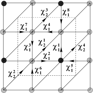
FIG. 11.: The $2\times 2$-site unit cell of the SU(N) Hubbard-Heisenberg model on the anisotropic triangular lattice. Arrows denote the orientation of the complex-valued $\chi_{\bf ij}$ fields.

Away from the pure Heisenberg limit $t_{1}=t_{2}=0$ we further classify the saddle-point solutions in terms of whether or not they break time-reversal symmetry ($\hat{T}$). Finally, as there are four independent parameters ($t_{1}$, $t_{2}$, $J_{1}$, and $J_{2}$) the phase diagram lives in a three-dimensional space of their dimensionless ratios. To reduce this to a more manageable two-dimensional section, we assume that $J_{1}/J_{2}=(t_{1}/t_{2})^{2}$; then by varying $J_{1}$ and the two hopping matrix elements we explore a two-dimensional space. The resulting phase diagram is shown in figure 12. We summarize the phases which appear in the diagram in the following subsections.

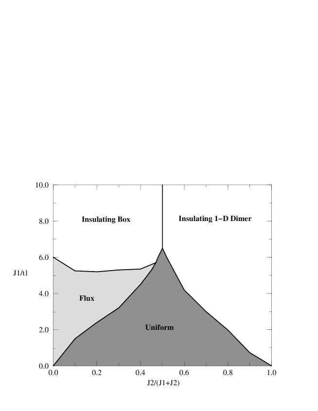
FIG. 12.: The zero temperature phase diagram of the SU(N) Hubbard-Heisenberg model on the anisotropic triangular lattice. The metallic uniform region is indicated by dark shading while light shading demarks the semi-metallic staggered flux phase.

1 One-Dimensional Dimer Phase

This phase exists in the region $J_{2}>J_{1}>t_{1}$ and it exhibits spin-Peierls (= dimer) order. All $\chi_{2}$-fields are negative real numbers with $\chi_{2}^{1}=\chi_{2}^{3}$, $\chi_{2}^{2}=\chi_{2}^{4}$, and $|\chi_{2}^{1}|>|\chi_{2}^{2}|$. Also, all $\chi_{1}$-fields are either small negative real numbers or zero with $\chi_{1}^{1}=\chi_{1}^{3}=\chi_{1}^{5}=\chi_{1}^{7}<0$, $\chi_{1}^{2}=\chi_{1}^{4}=\chi_{1}^{6}=\chi_{1}^{8}=0$ and $|\chi_{1}^{1}|\ll|\chi_{2}^{2}|$. See figure 13 for a sketch. The system breaks up into nearly decoupled dimerized spin chains. This phase breaks preserves $\hat{T}$-symmetry as all the $\chi$-fields are real. It is insulating as there is a large gap in the energy spectrum at the Fermi energy. The phase is very similar to the decoupled chain phase of the insulating Sp(N) model; in fact the dimerization pattern is identical to one of two such possible patterns in the Sp(N) model (see figure 4) and echos the pattern found by White and Affleck for the two-chain zigzag model[21]. In the extreme one-dimensional limit of $J_{1}=t_{1}=0$ the SU(N) solution, like the Sp(N) solution, fails[11] to accurately described the physics of decoupled chains, for at half-filling, the physical one-dimensional SU(2) Hubbard model is neither dimerized nor spin-gapped. The inclusion of the biquadratic interaction suppresses dimerization[38] and yields a state qualitatively similar to the exact solution of the physical system, but for simplicity we do not consider such a term here.

FIG. 13.: One-dimensional dimer phase. Dark lines indicate bonds with strong spin-spin correlations. These are the dimers.

2 Box (also called “Plaquette”) Phase

This phase is also insulating and consists of isolated plaquettes with enhanced spin-spin correlations[39, 30]. See figure 14 for a sketch. All $\chi_{1}$-fields are complex with $|\chi_{1}^{1}|=|\chi_{1}^{3}|>|\chi_{1}^{2}|=|\chi_{1}^{4}|>|\chi_{1}^{6}|=|\chi_{1}^{8}|>|\chi_{1}^{5}|=|\chi_{1}^{7}|$. The $\chi_{2}$ fields are small, $|\chi_{2}^{1}|=|\chi_{2}^{2}|=|\chi_{2}^{3}|=|\chi_{2}^{4}|\ll|\chi_{1}^{5}|$. The phase $\theta$ of the plaquette product $\chi_{1}^{1}\chi_{1}^{2}\chi_{1}^{3}\chi_{1}^{4}$ is neither 0 nor $\pi$ in general. The box phase breaks $\hat{T}$-symmetry when $t_{1}\neq 0$. As time-reversal symmetry is broken, there are real orbital currents circulating around the plaquettes[40] as shown in the figure. Apart from $\hat{T}$-breaking, this phase is rather similar to the $(\pi,\pi)$ SRO phase of the Sp(N) model as it is a commensurate SRO phase with a large spin gap.

FIG. 14.: Box (or “plaquette”) phase with circulating currents.

3 Staggered Flux Phase (SFP)

All $\chi_{1}$-fields are equal, with an imaginary component, and the $\chi_{2}$-fields are equal, real, and much smaller in magnitude than the $\chi_{1}$ fields. The phase of the plaquette operator differs in general from 0 or $\pi$; see figure 15 for a sketch. The staggered flux phase breaks $\hat{T}$-symmetry. Like the box phase, there are real orbital currents circulating around the plaquettes[40], in an alternating antiferromagnetic pattern. The SFP is semi-metallic as the density of states (DOS) is small, and in fact vanishes linearly at the Fermi energy at $J_{2}=0$. Apart from $\hat{T}$-breaking this phase is rather similar to the $(\pi,\pi)$ LRO phase of the Sp(N) antiferromagnet, as the spins show quasi-long-range order with power-law decay in the spin-spin correlation function. In the limiting case of a pure Heisenberg AF on the nearest-neighbor square lattice, $t_{1}=t_{2}=J_{2}=0$, gauge fluctuations at sufficiently small-N are expected to drive the SFP (which can be stabilized against the box phase by the addition of the biquadratic interaction) into a $(\pi,\pi)$ Néel-ordered state[41].

FIG. 15.: Staggered flux phase (SFP) with circulating currents.

4 Uniform Phase

All $\chi$-fields are negative real numbers and $\chi_{1}^{1}=\chi_{1}^{2}=\cdots=\chi_{1}^{8}$, $\chi_{2}^{1}=\chi_{2}^{2}=\chi_{2}^{3}=\chi_{2}^{4}$ with $\chi_{1}^{1}\neq\chi_{2}^{1}$ in general. See figure 16 for a sketch. This phase preserves $\hat{T}$-symmetry and since all $\chi$-fields are real, they simply renormalize hopping parameters $t_{1}$, $t_{2}$. The uniform phase is therefore a metallic Fermi liquid. Spin-spin correlations in the uniform phase decay as an inverse power law of the separation, with an incommensurate wavevector, so the uniform phase behaves similarly to that in the $(q,q)$ LRO phase of the Sp(N) model (see below).

FIG. 16.: Uniform phase with no broken symmetries. The uniform phase is a Fermi liquid.

C Global Similarities Between SU(N) and Sp(N) Phase Diagrams

There are some global similarities between the SU(N) phase diagram of the Hubbard-Heisenberg model (figure 12) and the Sp(N) phase diagram of the insulating Heisenberg antiferromagnet (figure 4). We have already pointed out similarities between the four phases of the SU(N) model and the decoupled chain, $(\pi,\pi)$ SRO, $(\pi,\pi)$ LRO, and $(q,q)$ LRO phases of the Sp(N) model. Apparently the dimensionless parameter $J_{1}/t_{1}$ on the vertical axis of the SU(N) phase diagram (figure 12) is the analog of the quantum parameter $1/\kappa$ of the Sp(N) phase diagram. The reason why these two dimensionless parameter play similar roles can be understood by considering the limit of the pure insulating antiferromagnet, corresponding to $t_{1}\rightarrow 0$ and $t_{2}\rightarrow 0$. In these limits, the SU(N) model can only be in the purely insulating box phase, or in the dimerized phase. The spins are always quantum disordered, and behave like the extreme quantum $\kappa\rightarrow 0$ limit of the Sp(N) model. In the opposite limit $t_{1}\rightarrow\infty$ and $t_{2}\rightarrow\infty$ the spin-spin correlation function decays more slowly, as an inverse power law instead of exponentially. This is as close to LRO as is possible in the large-N limit of the SU(N) model. Roughly then it corresponds to the ordered classical $\kappa\rightarrow\infty$ limit of the Sp(N) model.

D Observable Properties of the SU(N) Hubbard-Heisenberg Model

We now comment on the possible relevance of our large-N solution to the electronic and magnetic properties of the organic superconductors. In reference [3] it is estimated that $J_{2}/J_{1}\sim 0.3$ to $1$ and $J_{1}/t_{1}\sim 0.5$ to $2$. Figure 12 then implies that the ground state is the uniform phase, which as noted above, is a rather ordinary Fermi liquid with no broken symmetries.

We note that in the one-dimensional limit ($t_{1}=J_{1}=0$) and in the square lattice limit ($t_{2}=J_{2}=0$), nesting of the Fermi surface is perfect, and the system is driven into an insulating phase no matter how large the hopping amplitudes. Away from these two extreme limits, however, there is a non-trivial metal-insulator transition line. This accords with expectations because as the Fermi surface is not perfectly nested, the metallic state is only eliminated at a nonzero value of $J_{1}/t_{1}$. Experimentally it is found that upon increasing pressure, a SIT transition from the antiferromagnetic insulator to a superconductor is seen in the $\kappa$-(BEDT-TTF)₂X family of materials[35, 42]. This transition can be understood in terms of the SU(N) phase diagram as follows. As pressure increases, the effective hopping amplitudes $t_{1}$ and $t_{2}$ also increase because Coulomb blocking is less effective[3]. The bandwidth broadens, but the spin exchange couplings $J_{1}$ and $J_{2}$ remain nearly unchanged as these are determined by the bare, not the effective, hopping matrix elements. Thus the ratio $J_{1}/t_{1}$ is reduced at high pressure, and the many-body correlations weaken. From the phase diagram (figure 12) it is apparent that the system can be driven from an insulating state into a metallic state, which presumably superconducts at sufficiently low temperature. Thus the transition to a conducting state at high pressure can be seen as being due to bandwidth broadening, as in the Brinkman-Rice picture of the MIT.

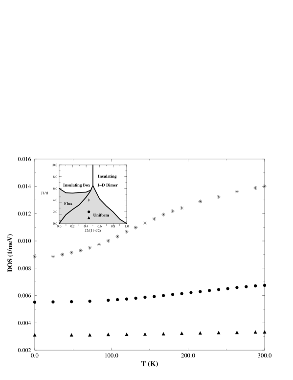
FIG. 17.: Density of states per unit volume at the Fermi energy as a function of temperature for three points, indicated by the inset and specified in table I, inside the uniform phase.

TABLE I.: Parameters (in meV) for the three points in figure 17.

Symbol In Figure 17	$t_{1}$	$t_{2}$	$J_{1}$	$J_{2}$	$J_{1}/t_{1}$	$J_{2}/(J_{1}+J_{2})$
star	6	5.4	24	19.2	4	0.44
dot	12	10.8	24	19.2	2	0.44
triangle	24	21.6	24	19.2	1	0.44

We plot the DOS as a function of temperature in figure 17 for three points inside the uniform phase identified in table I. The DOS decreases as the temperature decreases from room temperature down to absolute zero. Clearly the pseudogap is more prominent near the boundary between the conducting uniform phase and the semimetallic SFP and insulating box phases. The drop in the DOS could qualitatively explain the $30\%$ depression seen in the uniform susceptibility[35] (NMR experiments find a reduction of about $50\%$ as the temperature decreases from $100~{}^{\circ}$K to $10~{}^{\circ}$K[6, 7]). The behavior may be understood as follows. As the temperature decreases, antiferromagnetic spin-spin correlations develop. These correlations are signaled in the mean-field theory by the link variables $\chi_{\bf ij}$ which become non-zero at low enough temperature. Electrons on neighboring sites then tend to have opposite spin, reducing Pauli-blocking, and making their kinetic energy more negative. The band widens and the density of states drops.

V Discussion

We have solved the bosonic Sp(N) Heisenberg and fermionic SU(N) Hubbard-Heisenberg models on the anisotropic triangular lattice in the large-N limit. The bosonic Sp(N) representation of the Heisenberg model is useful for describing magnetic ordering transitions. It therefore may be an appropriate description of the insulating phase of the layered organic superconductors $\kappa$-(BEDT-TTF)₂X and of the insulating Cs₂CuCl₄ compound. The fermionic SU(N) Hubbard-Heisenberg model provides a complementary description of the charge sector, in particular the physics of metal-insulator transitions and the unconventional metallic phases. Systematic expansions in powers of $1/N$ about the large-N limit are possible for either model.

For the Sp(N) model we found five phases: (i) three commensurate phases, the $(\pi,\pi)$ LRO and SRO phases, and the decoupled chain phase and (ii) two incommensurate phases, the $(q,q)$ LRO and SRO phases. Passing from the square lattice ($J_{2}=0$) to the one-dimensional limit ($J_{1}=0$) at $\kappa=1$ which corresponds to spin-1/2 in the physical Sp(1) limit first there is the Néel ordered phase, the incommensurate $(q,q)$ LRO phase, the incommensurate $(q,q)$ SRO phase, and finally a phase consisting of decoupled chains. These phases are similar to those obtained from a series expansion method[31] and a weak coupling renormalization group technique[33]. The effects of finite-N fluctuations on the saddle-point solutions were also discussed. The observed dispersion of spin excitations in the Cs₂CuCl₄ material[34] can be described either as spinwaves in the incommensurate $(q,q)$ LRO phase, or in terms of pairs of spinons in the deconfined $(q,q)$ SRO phase.

The zero-temperature phase diagram of the SU(N) Hubbard-Heisenberg model in the large-N limit has a 1-D dimer phase, a box (or plaquette) phase, a staggered-flux phase, and a uniform phase. In the extreme 1-D and square lattice limits, the ground state of the half-filled Hubbard-Heisenberg model is always insulating because the nesting of the Fermi surface is perfect. But away from these two extreme limits there is a metal-insulator transition. For parameters appropriate to the $\kappa$-(BEDT-TTF)₂X class of materials we find that the conducting regime is described by our uniform phase, which is a rather conventional Fermi liquid with no broken symmetries. In this phase we find that the density of states at Fermi level decreases at low temperatures, due to the development of antiferromagnetic correlations. This could explain the depression seen in the uniform susceptibility of the organic superconducting materials at low temperatures. It agrees qualitatively with experiments which suggest the existence of a pseudo-gap.

We have used two models instead of one because the two large-N theories have complementary advantages and disadvantages. The bosonic Sp(N) approach is not suitable for describing electronic properties, as there are no fermions. The fermionic SU(N) approach, on the other hand, is not useful for describing magnetic ordering, as the order parameters are all SU(N) singlets. Neither mean-field approximation can describe the superconducting phase. The fermionic Sp(N) Hubbard-Heisenberg model does support superconducting states, but no non-superconducting metallic phases[37]. Whether or not a single model can be constructed which is exact in a large-N limit and yet encompasses all the relevant phases remains an open problem.

- [1] T. Ishiguro, K. Yamaji, and G. Saito, Organic Superconductors, Second Edition (Springer, Berlin, 1998).
- [2] J. Wosnitza, Fermi Surfaces of Low Dimensional Organic Metals and Superconductors (Springer, Berlin, 1996).
- [3] R. H. McKenzie 1998 Comments Cond. Matter Phys. 18 309.
- [4] H. Ito et al. 1996 J. Phys. Soc. Japan 65 2987.
- [5] T. Komatsu et al. 1996 J. Phys. Soc. Japan 65 1340.
- [6] S. M. De Soto et al. 1995 Phys. Rev. B52 10364.
- [7] H. Mayaffre, P. Wzietek, D. Jérome, C. Lenoir, and P. Batail, Europhys. Lett. 1994 28, 205.
- [8] N. Read and S. Sachdev 1991 Phys. Rev. Lett. 66 1773; S. Sachdev and N. Read 1991 Int. J. Mod. Phys. B5 219.
- [9] S. Sachdev, in Low Dimensional Quantum Field Theories for Condensed Matter Physicists, edited by Y. Lu, S. Lundqvist, and G. Morandi, (World Scientific, Singapore, 1995).
- [10] I. Affleck and J. B. Marston 1988 Phys. Rev. B37, 3774.
- [11] J. B. Marston and I. Affleck 1989 Phys. Rev. B39 11538.
- [12] A. Auerbach 1994 Interacting Electrons and Quantum Magnetism (Springer - Verlag, New York).
- [13] A. Fortunelli and A. Painelli 1997 J. Chem. Phys. 106 8051.
- [14] Y. Okuno and H. Fukutome 1997 Solid State Commun. 101 355.
- [15] F. Castet, A. Fritsch, and L. Ducasse 1996 J. Phys. I France 6 583.
- [16] A. E. Trumper 1999 Phys. Rev. B60 2987.
- [17] J. Merino, R. H. McKenzie, J. B. Marston, C. H. Chung 1999 J. Phys.: Condens. Matter 11 2965.
- [18] P. W. Anderson 1973 Mater. Res. Bull. 8 153.
- [19] L. Capriotti, A. Trumper, S. Sorella 1999 Phys. Rev. Lett. 82 3899, and references therein.
- [20] K. Okamoto and K. Nomura 1992 Phys. Lett. A169 433.
- [21] S. R. White and I. Affleck 1996 Phys. Rev. B54 9862.
- [22] S. Sachdev 1992 Phys. Rev. B45 12377.
- [23] William H. Press, Saul A. Teukolsky, William T. Vetterling, and Brian P. Flannery 1992 Numerical Recipes in C: The Art of Scientific Computing, Second Edition, pp. 451 – 455 (Cambridge University Press, New York, NY).
- [24] N. Read and S. Sachdev 1990 Phys. Rev. B42 4568.
- [25] E. Fradkin and S.H. Shenker 1979 Phys. Rev. D 19 3682.
- [26] A. V. Chubukov, S. Sachdev, and T. Senthil 1994 Nucl. Phys. B 426 601.
- [27] We thank S. Sachdev for emphasizing these differences.
- [28] R. Moessner and S. L. Sondhi, “An RVB phase in the triangular lattice quantum dimer model,” cond-mat/0007378.
- [29] D. Rokhsar and S. Kivelson 1988 Phys. Rev. Lett. 61, 2376; N. Read and B. Chakraborty 1989 Phys. Rev. B 40, 7133; X. G. Wen 1991 Phys. Rev. B 44, 2664; T. Senthil and M. P. A. Fisher 2000 Phys. Rev. B 62, 7850; G. Misguich and C. Lhuillier, “Some remarks on the Lieb-Schultz-Mattis theorem and its extension to higher dimension,” cond-mat/0002170.
- [30] C. H. Chung, J. B. Marston, and S. Sachdev, “Quantum phases of the Shastry-Sutherland Antiferromagnet,” cond-mat/0102222.
- [31] Z. Weihong, R. H. McKenzie and R.R.P. Singh 1999 Phys. Rev. B59 14367.
- [32] L. O. Manuel and H. A. Ceccatto 1999 Phys. Rev. B60 9489.
- [33] S.-W. Tsai and J.B. Marston, “Weak coupling renormalization-group analysis of two-dimensional Hubbard models: application to high- and -(BEDT-TTF)2X organic superconductors,” cond-mat/0010300.
- [34] R. Coldea, D.A. Tennant, A.M. Tsvelik, and Z. Tylczynski, 2001 Phys. Rev. Lett.86, 1335.
- [35] K. Kanoda 1997 Physica C 282 299.
- [36] J. B. Marston and C. Zeng, 1991 Journal of Applied Physics 69, 5962 – 5964 .
- [37] M. Vojta, Y. Zhang, and S. Sachdev 2000 Phys. Rev. B62 6721.
- [38] Matthew Hastings, private communication.
- [39] T. Dombre and G. Kotliar 1989 Phys. Rev. B38 855.
- [40] T. C. Hsu, J. B. Marston, and I. Affleck 1991 Phys. Rev. B43, 2866; D. A. Ivanov, Patrick A. Lee, and Xiao-Gang Wen 2000 Phys. Rev. Lett. 84, 3958; P. W. Leung 2000 Phys. Rev. B62, R6112; S. Chakravarty, R. B. Laughlin, D. K. Morr, and C. Nayak, “Hidden Order in the Cuprates,” cond-mat/0005443 (to appear in Phys. Rev. B); D. J. Scalapino, S. R. White, and I. Affleck, “Rung-Rung Current Correlations on a 2-Leg t-J Ladder,” cond-mat/0102182; J. B. Marston and Asle Sudbø, “Staggered Orbital Currents in a Model of Strongly Correlated Electrons,” cond-mat/0103120.
- [41] J. B. Marston 1990 Phys. Rev. Lett. 64, 1166; D. H. Kim and P. A. Lee 1999 Annals. Phys. 272, 130.
- [42] H. Kino and H. Fukuyama 1996 J. Phys. Soc. Japan 65 2158.