The Dynamics of Efficiency: A Simple Model

Abstract

We propose a simple model that describes the dynamics of efficiencies of competing agents. Agents communicate leading to increase of efficiencies of underachievers, and an efficiency of each agent can increase or decrease irrespectively of other agents. When the rate of deleterious changes exceeds a certain threshold, the economy falls into a stagnant phase. In the opposite situation, the economy improves with asymptotically constant rate and the efficiency distribution has a finite width. The leading algebraic corrections to the asymptotic growth rate are also computed.

PACS numbers: 05.40.-a, 05.70.Ln, 87.23.Ge

Non-equilibrium statistical mechanics is being increasingly applied to diverse fields outside physics, ranging from biology and computer science to finance and social science[1, 2, 3]. Indeed, the framework of non-equilibrium statistical mechanics is ideally suited for describing systems composed of many units that interact according to simple rules and exhibit a complex large-scale behavior. Thus, the important task is to construct simple stochastic models incorporating basic characteristics of the dynamics of systems under study which can then be analyzed by employing existing tools of non-equilibrium statistical mechanics. The hope is that these models can reproduce essential features of the original systems and can help to formulate relevant questions and enhance understanding of the dynamics of these systems.

In this paper, we propose a simple model that mimics the dynamics of efficiencies of competing agents. These agents could be airlines, travel agencies, insurance companies, etc. In today’s competing global economy, the performance of a company is continuously judged in the market and the index of performance depends on how efficient the company is. Rather than trying to incorporate all details of performances of competing agents, we choose a model that accounts for the dynamics of efficiency in the simplest form. We represent the efficiency of each agent by a single nonnegative number. The efficiency of every agent can, independent of other agents, increase or decrease stochastically by a certain amount which we set equal to unity. In addition, the agents interact with each other which is the fundamental driving mechanism for economy. We assume that the interaction equates the efficiencies of underachievers to the efficiencies of better performing agents.

The efficiency model formalizing the above features is defined as follows. Let $h_{i}(t)$ is the efficiency of agent $i$ at time $t$. Efficiencies $h_{i}$’s are non-negative integer numbers which evolve stochastically. Specifically, in an infinitesimal time interval $\Delta t$, every $h_{i}(t)$ can change as follows:

• $h_{i}(t)\to{\rm max}[h_{i}(t),h_{j}(t)]$ with probability $\Delta t$, where the agent $j$ is chosen randomly. This move is due to the fact that each agent tries to equal its efficiency to that of a better performing agent in order to stay competitive.

• $h_{i}(t)\to h_{i}(t)+1$ with probability $p\Delta t$. This incorporates the fact that each agent can increase its efficiency, say due to innovations, irrespective of other agents.

• $h_{i}(t)\to h_{i}(t)-1$ with probability $q\theta(h_{i}(t))\Delta t$, where $\theta(x)$ is the Heaviside step function. This corresponds to the fact that each agent can loose its efficiency due to unforeseen problems such as labour strikes. Note, however, that since $h_{i}(t)\geq 0$, this move can occur only when $h_{i}(t)\geq 1$.

• With probability $1-[1+p+q\theta(h_{i}(t))]\Delta t$, the efficiency $h_{i}(t)$ remains unchanged.

This efficiency model exhibits rich phenomenology. In particular, the system undergoes a delocalization phase transition as the parameters $p$ and $q$ are varied. There exists a critical line $p_{c}(q)$ in the $(p,q)$ plane such that for $p>p_{c}(q)$, the average efficiency increases linearly with time, $\langle h\rangle\sim vt$ for large $t$. We shall determine exactly the rate $v(p,q)$ of the average efficiency growth. For $p\leq p_{c}(q)$, the economy is stagnant, i.e., the efficiency distribution becomes stationary in the large time limit. This delocalization (or depinning) phase transition is dynamical in nature and is different from the depinning transitions found in equilibrium systems with quenched disorder. Similar delocalization transitions have recently been found in a variety of non-equilibrium processes[4, 5, 6, 7, 8].

Let $P(h,t)$ denotes the fraction of agents with efficiency $h$ at time $t$. One can easily write down the evolution equation for $P(h,t)$ by counting all possible gain and loss terms. For $h\geq 1$, this equation reads

$${dP(h,t)\over dt}= - P(h,t)\sum_{h^{\prime}=h+1}^{\infty}P(h^{\prime},t)-(p+q)P(h,t)$$ (1)

$$+ qP(h+1,t)+pP(h-1,t)$$ (2)

$$+ P(h,t)\sum_{h^{\prime}=0}^{h-1}P(h^{\prime},t).$$ (3)

In writing Eq. (3), we have used the fact that when the total number of agents diverges, the joint probability distribution $P(h,h^{\prime},t)$ of two agents having efficiencies $h$ and $h^{\prime}$ factorises, $P(h,h^{\prime},t)=P(h,t)P(h^{\prime},t)$, and the mean-field theory becomes exact.

It proves convenient to consider the cumulative distribution, $F(h,t)=\sum_{h^{\prime}\geq h}P(h^{\prime},t)$. From Eq. (3), we immediately derive the evolution equation for $F(h,t)$,

$${dF(h,t)\over dt}= - F^{2}(h,t)+(1-p-q)F(h,t)$$ (4)

$$+ qF(h+1,t)+pF(h-1,t).$$ (5)

Note that this equation is valid for all $h\geq 1$ and by the probability sum rule we have $F(0,t)=1$ for arbitrary $t$. Also, $F(h,t)\to 0$ as $h\to\infty$ for all $t$.

Equation (5) is a nonlinear difference-differential equation and is, in general, hard to solve exactly. Fortunately, many asymptotic properties can be derived analytically without solving Eq. (5). First we note that $F(h,t)$ approaches a traveling wave form as it follows e.g. from direct numerical integration of Eq. (5). Thus, we seek a solution of the form $F(h,t)=f(h-vt)$. By inserting it into Eq. (5) we find that $f(x)$ satisfies

$$-v{{df}\over{dx}} = -f^{2}(x)+(1-p-q)f(x)$$ (6)

$$+ qf(x+1)+pf(x-1),$$ (7)

which should be solved subject to the boundary conditions $f(-\infty)=1$ and $f(\infty)=0$. To determine $v$, we linearize Eq. (7) in the tail region, $x\to\infty$. The resulting linear equation admits an exponential solution, $f(x)\sim\exp(-\lambda x)$. By inserting this asymptotics into the linearized version of Eq. (7) we find that the growth rate $v(\lambda)$ is related to the decay exponent $\lambda$ via

$$v(\lambda)={1-p-q+qe^{-\lambda}+pe^{\lambda}\over\lambda}.$$ (8)

Thus we have a family of eigenvalues parameterized by $\lambda$. According to a general selection principle which applies to a wide class of nonlinear equations[9, 10], only one specific rate out of this family of possible $v$’s is selected. Usually, the minimum rate is selected. For sufficiently steep initial conditions, the minimum rate is universal, while extended initial conditions might affect the magnitude of the admissible minimum rate.

The function $v(\lambda)$ in Eq. (8) has a unique minimum at $\lambda=\lambda^{*}$ given by the solution of ${{dv}\over{d\lambda}}=0$, or

$$1-p-q+qe^{-\lambda^{*}}+pe^{\lambda^{*}}=\lambda^{*}\left[-qe^{-\lambda^{*}}+pe^{\lambda^{*}}\right].$$ (9)

The corresponding minimum rate $v_{\rm min}(p,q)\equiv v(\lambda^{*})$ is given by Eq. (8), or

$$v_{\rm min}=-qe^{-\lambda^{*}}+pe^{\lambda^{*}}$$ (10)

as it follows from (9). An analysis of Eqs. (8)–(10) shows that there exists a critical line $p_{c}(q)$ in the $(p,q)$ plane,

$$p_{c}(q)=\cases{1+q-2\sqrt{q}&for $q\geq 1$,\cr 0&for $q\leq 1,$}$$ (11)

such that $v(\lambda)>0$ for all $\lambda\geq 0$ as long as $p>p_{c}(q)$. For a fixed $q$, as $p\to p_{c}(q)$ from above, $v_{\rm min}\to 0$ and for $0<p<p_{c}(q)$, the curve $v(\lambda)$ crosses zero at $\lambda=\lambda_{1}$ and $\lambda=\lambda_{2}$ with $\lambda_{2}>\lambda_{1}$. When $\lambda_{1}<\lambda<\lambda_{2}$, $v(\lambda)$ becomes negative. This tells that there might be no traveling wave solution for $0<p<p_{c}(q)$ and we anticipate that the efficiency distribution should become stationary. Note that for $q<1$, $p_{c}(q)=0$ and this regime does not occur.

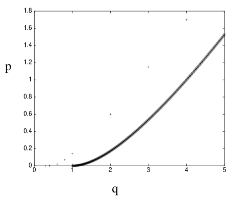
FIG. 1.: The thick line represents the critical locus, $p_{c}(q)=1+q-2\sqrt{q}$, for the mean-field theory. The $+$’s indicate numerically obtained critical points in one dimension. For sharply decaying initial conditions, the economy is developing when $p>p_{c}(q)$ and stagnant when $p\leq p_{c}(q)$.

With the above picture in mind, we now discuss the selection principle more carefully. Consider an exponentially decaying initial condition, $F(h,0)\sim e^{-\alpha h}$ with $\alpha>0$. When $p>p_{c}(q)$, the rate is positive for all $\lambda>0$ and $v(\lambda)$ has a unique minimum at $\lambda=\lambda^{*}$. Applying the selection principle we find that for sufficiently steep initial conditions, $\alpha>\lambda^{*}$, the selected growth rate is $v_{\rm min}=v(\lambda^{*})$. Consider now sufficiently extended initial conditions, $\alpha<\lambda^{*}$. In this case, $f(x)$ must decay at most as $e^{-\alpha x}$ and therefore the growth rate is selected among $v(\lambda)$, Eq. (8), with $\lambda\leq\alpha$. The selection principle now implies that the selected rate is $v=v(\alpha)$.

When $p\leq p_{c}(q)$, we must separately consider two cases: $q>1$ and $q\leq 1$. For $q>1$, $v(\lambda)$ as given by Eq. (8) becomes negative in the region $\lambda_{1}<\lambda<\lambda_{2}$. We find that for all $\alpha<\lambda_{1}$, the system still admits a traveling wave solution and the selected rate is $v=v(\alpha)$. However, for $\alpha>\lambda_{1}$, the system no longer admits a traveling wave solution. Instead, the distribution $F(h,t)$ reaches a stationary limit $P_{\infty}(h)$ as $t\to\infty$. By putting the time derivative equal to zero on the left-hand side of Eq. (5), we find that the stationary efficiency distribution decays exponentially, $F_{\infty}(h)\sim e^{-\mu h}$, with

$$\mu(p,q)=\ln\left[{-1+p+q+\sqrt{(1-p-q)^{2}-4pq}\over 2p}\right].$$ (12)

Note that $\mu(p,q)$ is real below the critical line, i.e., when $q>1$ and $p\leq p_{c}(q)$. Interestingly, $\mu(p,q)$ remains finite on the critical line $p=p_{c}(q)$. From Eqs. (12) and (11) we find that $\mu_{c}(q)=\mu(p_{c}(q),q)$ reads

$$\mu_{c}(q)=\ln\left({\sqrt{q}\over\sqrt{q}-1}\right).$$ (13)

For $q\leq 1$, $p_{c}(q)=0$. When $p\to 0$, we have $v_{\rm min}\to 0$ and $\lambda^{*}\to\infty$. The divergence of the decay exponent $\lambda^{*}$ indicates that when $p=0$ and $q<1$, the system still admits a traveling wave solution and the selected rate is $v=v(\alpha)$ if we start with an exponentially decaying initial condition, $F(h,0)\sim e^{-\alpha h}$. Of course, for compact initial conditions (i.e., when $F(h,0)=0$ for sufficiently large $h$), the efficiency distribution becomes stationary in the long time limit. We have verified all the above assertions via direct numerical integration of Eq. (5).

Although one cannot provide explicit expressions for the growth rate in the developing phase, near the critical line $p_{c}(q)$ the growth rate considerably simplifies. First we note that on general scaling grounds one would guess that above the critical line, the growth rate $v_{\rm min}(p,q)$ should be a function of $p-p_{c}$ with critical behavior

$$v_{\rm min}\sim(p-p_{c})^{\beta}.$$ (14)

The actual behavior is found by a straightforward analysis of Eqs. (8)–(9) to yield

$$v_{\rm min}\to\cases{{p-p_{c}(q)\over(\sqrt{q}-1)\mu_{c}(q)}&for $q>1$,\cr\cr{4\sqrt{p}\over\ln(1/p)}&for $q=1$,\cr\cr{1-q\over\ln(1/p)}&for $0\leq q<1$,\cr}$$ (15)

where $\mu_{c}(q)$ is given by Eq. (12). Equation (15) implies that the mobility exponent $\beta$ in the scaling relation (15) is equal to $1,1/2$ and $0$ for $q>1,q=1$ and $q<1$, respectively. In the last situation ($q<1$ and $p\to 0$), the growth rate still approaches to zero but it occurs in an extremely slow inverse logarithmic fashion.

The relaxation of the growth rate $v(t)$ towards its asymptotic value $v_{\rm min}$ exhibits an interesting algebraic behavior. Specifically, the leading correction is proportional to $t^{-1}$, the next is of order $t^{-3/2}$, etc. Similar $t^{-1}$ correction was first derived by Bramson in the context of a reaction-diffusion equation[10], and was subsequently re-derived and generalized by a number of authors[11, 12]. The next correction was recently derived by Ubert and van Saarloos[13]. In contrast to Refs.[10, 11, 12, 13], we consider the difference-differential equation. Fortunately, the techniques[10, 11, 12, 13] still apply (compare [8, 14]), so we do not detail the derivation. Following for instance an approach of Ref.[13], one finds

$$v(t)=v_{\rm min}-{3\over 2\lambda^{*}}\,t^{-1}+A\,t^{-3/2}+{\cal O}(t^{-2}),$$ (16)

with $A=3\pi^{1/2}\{2(qe^{-\lambda^{*}}+pe^{\lambda^{*}})\}^{-1/2}(\lambda^{*})^{-2}$. The explicitly displayed terms are universal – they do not depend on initial condition as long as it is steep enough [i.e., it falls off faster than $e^{-\lambda^{*}x}$]. The following terms in Eq. (16) starting from ${\cal O}(t^{-2})$ correction are non-universal. Thus not only any sufficiently steep initial profile relaxes to a unique profile, the approach to that profile occurs along (asymptotically) unique trajectory. Note also that the very slow $t^{-1}$ relaxation of the growth rate leads to a logarithmic correction to the average efficiency,

$$\langle h\rangle=v_{\rm min}t-{3\over 2\lambda^{*}}\,\ln t+{\cal O}(1).$$ (17)

Thus, we have a delocalization transition across the critical line $p_{c}(q)$ in the $(p,q)$ plane for sharply decaying initial conditions. For such initial conditions, as long as $p>p_{c}(q)$, the economy is in the developing phase with the average efficiency increasing as $\langle h\rangle\approx v_{\rm min}t$, where the rate $v_{\rm min}$ given by Eqs. (10) and (9). For $p\leq p_{c}(q)$ with $q>1$, the system is localized and $\langle h\rangle$ approaches a time-independent constant in the long time limit. For $p=0$ and $q<1$, the economy is in the developing phase for unbounded initial efficiency distributions, with the rate of growth explicitly dependent on the initial condition. For economically more relevant compact initial conditions, the regime $p=0$ and $q<1$ belongs to the stagnant phase. These results are summarized in the phase diagram in Fig. 1.

The mean-field version of the efficiency model is natural in the interconnected modern economy. In economy with limited communication, however, the efficiency model in a low dimensional space rather than in the fully connected graph might be more appropriate. In this case, agents are placed on a finite dimensional lattice. The microscopic dynamical steps (i)–(iv) remain the same except that in move (i), the agent $j$ is chosen to be one of the nearest neighbors of $i$. Unlike the mean-field theory, the correlations between $h_{i}$’s at different sites remain nonzero in finite dimensions even in the thermodynamic limit. We have studied this model numerically in one dimension. The results are shown for lattice size $L=1000$ (we verified that for such large systems, the finite size effect is insignificant). Once again, there is a delocalization transition in the $(p,q)$ plane across a critical line as shown in Fig. 1. The efficiency distribution $P(h,t)$ at different times in both phases is presented in Fig. 2.

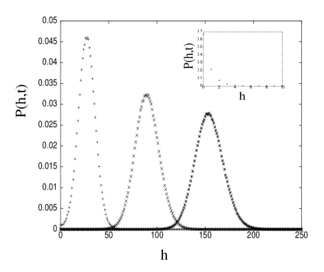
FIG. 2.: The distribution $P(h,t)$ at times $t=200$, $600$ and $1000$ in the moving phase for $p=3$, $q=4$. The inset shows the distribution at the same times in the localized phase for $p=1$, $q=4$. For $q=4$, the critical point is $p_{c}(q)\approx 1.7$.

We now stress important differences between mean-field and finite-dimensional situations. In the former case the nature of the two phases depends on the steepness parameter $\alpha$, while in one dimension the nature of the final state is independent of $\alpha$. For example, in the developing phase the system always has a traveling wave solution with a rate that depends on $p$ and $q$ but does not depend on $\alpha$. We have tested this fact numerically for several values of $\alpha$. This result is rather counter intuitive as it suggests that correlations seem to restore universality that mean-field theory lacks. Another important distinction is a very different behavior of the width of the efficiency distribution in the developing phase. Indeed, in mean-field the width is constant, while in one dimension it increases with time [see Fig. 2]. Moreover, the width increases as a power law, $w=\sqrt{\langle h^{2}\rangle-\langle h\rangle^{2}}\sim t^{\beta}$ for large $t$, with $\beta\approx 0.31$ in $(1+1)$ dimensions.

In $(d+1)$-dimensions, one can interpret the efficiency $h_{i}(t)$ as the height of a surface growing on a $d$-dimensional substrate. In this language, our efficiency model represents a continuous time polynuclear growth (PNG) model with additional adsorption and desorption rates[15]. The continuous PNG model without desorption has been studied within mean-field theory[16] and was found to be always in the moving phase as expected. From the general analogy to PNG models, we expect that the moving phase in the efficiency model corresponds to a growing interface belonging to the Kardar-Parisi-Zhang (KPZ) universality class[15]. The numerically obtained width exponent $\beta\approx 0.31$ in $(1+1)$-dimensions is consistent with the KPZ prediction $\beta=1/3$. It would be interesting to determine the universality class of the delocalization transition. Phase transitions in several PNG models in $(1+1)$-dimensions belong to the directed percolation (DP) universality class (see e.g. Ref.[17]). Other similar growth models exhibit phase transitions that do not belong to the DP universality class[4, 6]. It remains an open question whether the phase transition in the efficiency model in $(1+1)$-dimensions belong to the DP universality class.

In summary, we have investigated a simple model of the dynamics of efficiencies of competing agents. The model takes into account stochastic increase and decrease of the efficiency of every agent, independent of other agents, and interaction between the agents which equates the efficiencies of underachievers to that of better performing agents. We have shown that the model displays a phase transition from stagnant to growing economy.

One of us (PLK) acknowledges support from NSF (grant DMR9978902) and ARO (grant DAAD19-99-1-0173).

REFERENCES

- [1] M. S. Waterman, Introduction to Computational Biology: Maps, Sequences and Genomes (Chapman and Hall, London, 1995).
- [2] R. N. Mantegna and H. E. Stanley, An Introduction to Econophysics: Correlations and Complexity in Finance (Cambridge University Press, New York, 2000).
- [3] R. Axelrod, The Complexity of Cooperation (Princeton University Press, Princeton, 1997).
- [4] H. Hinrichsen, R. Livi, D. Mukamel, and A. Politi, Phys. Rev. Lett. 79, 2710 (1997).
- [5] T. Hwa and M. Munoz, Europhys. Lett. 41, 147 (1998).
- [6] S. N. Majumdar, S. Krishnamurthy, and M. Barma, Phys. Rev. E 61, 6337 (2000).
- [7] L. Giada and M. Marsili, Phys. Rev. E 62, 6015 (2000).
- [8] S. N. Majumdar and P. L. Krapivsky, Phys. Rev. E 62, 7735 (2000).
- [9] J. D. Murray, Mathematical Biology (Springer-Verlag, New York, 1989).
- [10] M. Bramson, Convergence of Solutions of the Kolmogorov Equation to Travelling Waves (American Mathematical Society, Providence, R.I., 1983).
- [11] W. van Saarloos, Phys. Rev. A 39, 6367 (1989).
- [12] E. Brunet and B. Derrida, Phys. Rev. E 56, 2597 (1997).
- [13] U. Ebert and W. van Saarloos, Phys. Rev. Lett. 80, 1650 (1998); Physica D 146, 1 (2000).
- [14] P. L. Krapivsky and S. N. Majumdar, Phys. Rev. Lett. 85, 5492 (2000).
- [15] A review of surface growth, and in particular PNG model, is given by T. Halpin-Healy and Y.-C. Zhang, Phys. Reports 254, 215 (1995).
- [16] E. Ben-Naim, A. R. Bishop, I. Daruka, and P. L. Krapivsky, J. Phys. A 31, 5001 (1998).
- [17] J. Kertesz and D. E. Wolf, Phys. Rev. Lett. 62, 2571 (1989).