Numerically improved computational scheme for the optical conductivity tensor in layered systems

Abstract

The contour integration technique applied to calculate the optical conductivity tensor at finite temperatures in the case of layered systems within the framework of the spin–polarized relativistic screened Korringa–Kohn–Rostoker band structure method is improved from the computational point of view by applying the Gauss–Konrod quadrature for the integrals along the different parts of the contour and by designing a cumulative special points scheme for two–dimensional Brillouin zone integrals corresponding to cubic systems.

1 Introduction

Nowadays magneto-optical effects are widely used to probe the magnetic properties of various systems [1, 2, 3]. For a theoretical description of these effects, one needs to calculate the optical conductivity tensor in a parameter–free manner. Recently, two of the authors have proposed a new, contour integration technique to calculate the optical conductivity tensor for surface layered systems [4]. The theoretical framework of the present paper is based on this technique. Therefore, in the following the basic concepts of this method are only briefly reviewed.

The starting point of the contour integration technique is the expression for the optical conductivity tensor

$$\Sigma_{\mu\nu}(\omega)=\dfrac{\sigma_{\mu\nu}(\omega)-\sigma_{\mu\nu}(0)}{\hbar\omega+i\delta}$$ (1)

as given by Luttinger [5], where $\omega$ denotes the photon frequency and $\delta$ a finite life–time broadening, respectively. The latter accounts for those scattering processes, which are not incorporated in a standard band structure calculation, but are present at finite temperatures.

The temperature $T$ enters the expression for the zero wavenumber current–current correlation function parametrically [6]

$$\sigma_{\mu\nu}(\omega)=\dfrac{i\hbar}{V}\,\sum_{m,n}\dfrac{f(\epsilon_{n})-f(\epsilon_{m})}{\hbar\omega+i\delta+(\epsilon_{n}-\epsilon_{m})}\,J^{\mu}_{nm}J^{\nu}_{mn}$$ (2)

via the Fermi–Dirac distribution function $f(\epsilon)$, with $\epsilon_{m}$ and $\epsilon_{n}$ being the eigenvalues of the one–electron Hamiltonian corresponding to states labeled by $m$, $n$ and the $J^{\mu}_{nm}$ $(\mu=\mathrm{x,y})$ the current matrices. In Ref. [4] it was shown, that Eq. (2) can be evaluated by means of a contour integration using complex energy values $z$. Within this technique, $\sigma_{\mu\nu}(\omega)$ is decomposed into a contour path contribution $\sigma^{(\mathrm{C})}_{\mu\nu}(\omega)$ and a contribution, $\sigma^{(\mathrm{M})}_{\mu\nu}(\omega)$, arising from the Matsubara poles $\sigma^{(\mathrm{M})}_{\mu\nu}(\omega)$, such that

$$\sigma_{\mu\nu}(\omega)=\sigma^{(\mathrm{C})}_{\mu\nu}(\omega)+\sigma^{(\mathrm{M})}_{\mu\nu}(\omega)\,.$$ (3)

As shown in Fig. 1, $\sigma^{(\mathrm{C})}_{\mu\nu}(\omega)$, in turn, consists of the contributions from the contour in the upper and lower semi–plane as given by Eqs. (24) and (25) in Ref. [4]. One contribution to $\sigma^{(\mathrm{M})}_{\mu\nu}(\omega)$ comes from the $n_{2}$ Matsubara poles near and on both sides of the real axis, and an other one from the $n_{1}$ poles situated exclusively in the upper semi–plane, see Eq. (26) in Ref. [4]. (Note that according to Ref. [4], $n_{1}=N_{1}-N_{2}$ and $n_{2}=N_{2}$.) Each of these contributions (altogether four) is expressed in terms of

$$\tilde{\sigma}_{\mu\nu}(z_{1},z_{2})=-\dfrac{\hbar}{2\pi V}\,\mathrm{Tr}\,\left[J^{\mu}G(z_{1})J^{\nu}G(z_{2})\right]\,,$$ (4)

where $J^{\mu}$ and $G(z_{i})$ denote current operators and resolvents, respectively. Application of this contour integration technique to compute $\Sigma_{\mu\nu}(\omega)$ for ordered or disordered (within the framework of the single site Coherent Potential Approximation) layered systems is therefore straightforward [7]. Originally, the quantities $\tilde{\sigma}_{\mu\nu}(z_{1},z_{2})$ were introduced to facilitate the computation of the dc conductivity based on the Kubo–Greenwood formalism [8, 9] in case of substitutionally disordered bulk systems [10].

In the present paper, the Green functions $G(z)$ entering Eq. (4) are calculated by means of the spin–polarized relativistic screened Korringa–Kohn–Rostoker (SKKR) method for layered systems [11, 12, 13] and the matrix elements $J^{\mu}_{mn}$ ($\mu=\mathrm{x,y}$) using the relativistic current operator [7]. Because of the non–vanishing imaginary part of the complex energies $z$ (see Fig. 1), also the so–called irregular solutions of the Dirac equation have to be considered [4].

To start a computation of the optical conductivity tensor $\Sigma_{\mu\nu}(\omega)$ for a given frequency $\omega$ and temperature $T$, the self–consistently determined potentials of the investigated layered system must be known. This means that the bottom energy $\epsilon_{\mathrm{b}}$ and the Fermi level $\epsilon_{\mathrm{F}}$ are also known. Thus $\min(\mathrm{Re}\,z)$ is fixed at $\epsilon_{\mathrm{b}}$ and $\max(\mathrm{Re}\,z)$ at $\epsilon_{\mathrm{F}}+mk_{\mathrm{B}}T$ ($m\in\mathbb{N}$, $k_{\mathrm{B}}$ the Boltzmann constant). Due to the fast decay of the Fermi–Dirac distribution function, at a given $T$ the computed optical conductivity tensor depends only slightly on the used value of $m$. The results given in the present paper were obtained with $m=8$. As can be seen from Fig. 1, the value of $\mathrm{Im}\,z$ is $\delta_{1}$ in the upper and $\delta_{2}$ in the lower semi–plane along the contour part parallel to the real axis. Taking, $\delta_{j}=2n_{j}\delta_{T}$ ($j$=1,2), with $\delta_{T}=\pi k_{\mathrm{B}}T$, it is ensured that the paths parallel to the real axis fall in–between two successive Matsubara poles [4].

In order to make use of the symmetry properties of the $\tilde{\sigma}_{\mu\nu}(z_{1},z_{2})$ in Eq. (4), for the life–time broadening a value of $\delta=2\delta_{2}$ has been chosen. An other advantage of this set–up is that for example at $T$ = 300 K and $\delta\approx$ 0.05 Ryd, one needs only $n_{2}=2$ Matsubara poles.

The computed value of the optical conductivity $\Sigma_{\mu\nu}(\omega)$ depends strongly on the number of complex energy points used on different parts of the contour in both semi–planes: quarter circle, parallel to the real axis and in the vicinity of the Fermi level. Furthermore, the number of $\vec{k}$–points used to calculate the scattering path operator and $\tilde{\sigma}_{\mu\nu}(z\pm\hbar\omega+i\delta,z)$ at a given energy $z$, (see Eqs. (53) and (54) from Ref. [7]), is of crucial importance.

The aim of the present paper, is to describe efficient numerical methods to control the accuracy of the contour and $\vec{k}$–space integrations without increasing the computational effort: in Section 2 Konrod’s extension to the Gauss quadrature as a proper numerical method is discussed; in Section 3 a new, cumulative special points method is presented to compute two–dimensional $\vec{k}$–space integrals with arbitrary high precision. Finally, the independence of $\Sigma_{\mu\nu}(\omega)$ on the contour path in the upper semi–plane, i.e. on the $n_{1}$ Matsubara poles, is shown separately in Section 4.

2 Contour integration by means of the Konrod–Legendre rule

The $n$–point Gauss–Legendre integration rule [14] can be used directly to compute $\sigma^{(\mathrm{C})}_{\mu\nu}(\omega)$ in Eq. (3) by transforming the nodes $x_{k}$ and their weights $w_{k}$ ($k=1,\ldots,n$) according to the different contour parts (Fig. 1). The nodes are roots of the Legendre polynomials $P_{n}(x)$ corresponding to the weighting function $w(x)=1$, $x\in(-1,1)$ and are usually computed using the Newton method [15]. For the weights $w_{k}$, one needs also to compute the derivatives of the $P_{n}(x)$ with respect to the argument $P_{n}^{\prime}(x_{k})$.

One way to estimate the accuracy is to repeat the above procedure for $n+1$ points and compare the results. This requires the evaluation of the integrand for all the newly generated $n+1$ complex energy points, because $P_{n+1}(x)$ has no common roots with $P_{n}(x)$ [14], which of course is computationally very inefficient.

In 1965 Konrod has proposed a method to overcome the above difficulty by demonstrating that one can create a set of $2n+1$ nodes including all the nodes of an $n$–point Gauss quadrature [16]. Furthermore, he also showed that each of the additional $n+1$ nodes falls in–between two nodes of the $n$–point Gauss quadrature. Thus, once the integrand $f(x)$ is evaluated for each of the $2n+1$ nodes, $\tilde{x}_{k}$, both the Gauss (denoted by $\mathcal{G}_{n}$)

$$\mathcal{G}_{n}f=\sum_{k=1}^{n}f(\tilde{x}_{2k})w_{2k}$$ (5)

and the Konrod sum (denoted by $\mathcal{K}_{2n+1}$)

$$\mathcal{K}_{2n+1}f=\sum_{k=1}^{2n+1}f(\tilde{x}_{k})\tilde{w}_{k}\,,$$ (6)

are available. Usually, the nodes $\tilde{x}_{k}$ and weights, $\tilde{w}_{k}$ and $w_{2k}$, are obtained from the spectral factorization of the associated Jacobi–Konrod (Jacobi–Gauss) matrix [17]. The Jacobi–Gauss matrix is formed easily knowing the recursion coefficients of those monic, orthogonal polynomials (say Legendre polynomials), which correspond to the weighting function (in our case the identity) [14]. But these coefficients fill only partially the Jacobi–Konrod matrix. Hence, to form the Jacobi–Konrod matrix is not a trivial task.

Laurie [18] was the first, who in 1997 developed an algorithm, based on the mixed moments method in order to generate the Jacobi–Konrod matrix for even $n$. Recently, Calvetti et al. [17] extended Laurie’s ideas to odd $n$ using a divide–and–conquer scheme.

We have implemented Laurie’s algorithm [18] to calculate the $2n+1$ recursion coefficients entering the Jacobi–Konrod matrix. The initialization requires $3n/2$ ($n$ even) elements of the Jacobi–Gauss matrix derived from a common set of monic, orthogonal polynomials. These are obtained using the algorithm described in Ref. [19]. The same Ref. [19] is then used to generate the nodes and weights for the Konrod rule and the weights for the Gauss rule with machine dependent accuracy, say $10^{-15}$. In contrast to the implementation of the Konrod rule described in Ref. [20], the present one works for arbitrary even $n$, i.e. $\mathcal{G}_{n}f$ can be compared with $\mathcal{K}_{2n+1}f$ not only for some particular values of $n$. The final result of the quadrature is then that obtained by means of the Konrod rule. Since $\sigma^{(\mathrm{C})}_{\mu\nu}(\omega)$ is not a scalar quantity for each pair of $(\mu,\nu)$, $\mathcal{G}_{n}\sigma_{\mu\nu}(\omega)\equiv\sigma^{(n)}_{\mu\nu}(\omega)$ is compared separately with $\mathcal{K}_{2n+1}\sigma_{\mu\nu}(\omega)\equiv\sigma^{(2n+1)}_{\mu\nu}(\omega)$. The integrand along a particular part of the contour, see Fig. 1, is said to be converged if the maximum difference

$$\max\mid\sigma^{(2n+1)}_{\mu\nu}(\omega)-\sigma^{(n)}_{\mu\nu}(\omega)\mid\;\leq\;\varepsilon_{z}\quad(\mu,\nu=\mathrm{x,y})\,,$$ (7)

where $\varepsilon_{z}$ is an arbitrary small number, e.g. machine accuracy ($10^{-15}$).

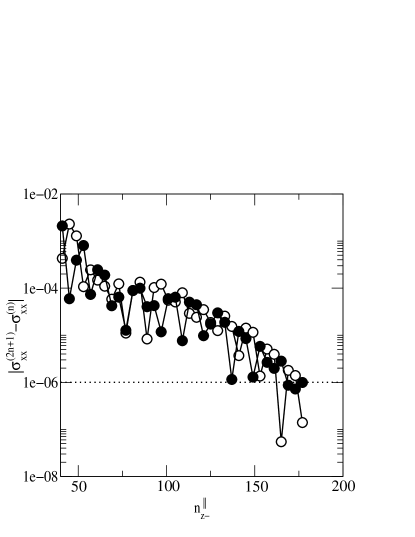
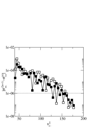
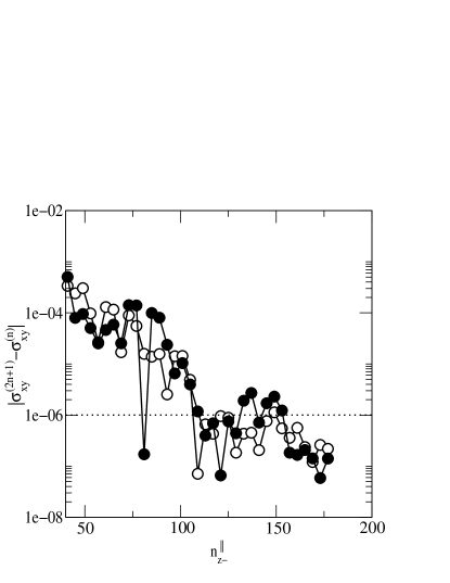
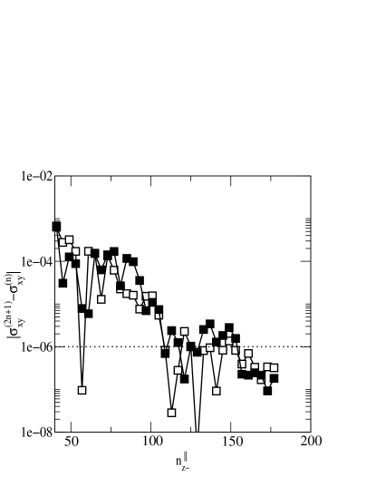
Figure 2: Absolute difference between $\sigma_{\mu\nu}^{(2n+1)}(\omega)$ and $\sigma_{\mu\nu}^{(n)}(\omega)$ (atomic units) versus the total number of complex energy points used parallel to the real axis in the lower semi–plane for $\hbar\omega$ = 0.05 Ryd and $T$ = 300 K. The real part in the difference of the regular (left panels) and irregular (right panels) contribution is given by open symbols ($\circ$, $\Box$) and the imaginary part by corresponding filled symbols ($\bullet$, $\blacksquare$), respectively. The dotted line marks a value of $10^{-6}$ in atomic units.)

In Fig. 2 $\mid\sigma^{(2n+1)}_{\mu\nu}(\omega)-\sigma^{(n)}_{\mu\nu}(\omega)\mid$ is plotted for $\hbar\omega$ = 0.05 Ryd and $T$ = 300 K versus the number of complex energy points $n_{z-}^{\parallel}$ used parallel to the real axis in the lower semi–plane. For all other parts of the contour, not shown here, the corresponding quantities $\mid\sigma^{(2n+1)}_{\mu\nu}(\omega)-\sigma^{(n)}_{\mu\nu}(\omega)\mid$, show an almost linear dependence on $n$. The rather complicated shape of the data displayed in Fig. 2 has a physical reason: in the lower semi–plane, near ($\delta_{2}$ = 0.024 Ryd) and parallel to the real axis mostly the joint density of states with all its singularities is mapped.

In the present paper, the layered system used for test calculations is a mono–layer of Co on the top of fcc–Pt(100), i.e. below the Co surface layer there are three Pt buffer layers followed by Pt bulk [21]. The band bottom energy ($\epsilon_{\mathrm{b}}$) and the Fermi level ($\epsilon_{\mathrm{F}}$) of the substrate corresponds to $-1$ and $-0.039$ Ryd, respectively. The optical conductivity calculation was carried out using $n_{1}$ = 18 and $n_{2}$ = 2 Matsubara poles. The number of $\vec{k}$–points within the surface Brillouin zone was 16 (further discussions on this point are made in Section 3). Analyzing the values obtained, it can be concluded that for the case chosen, the following set of numerical parameters

$$\begin{array}[c]{rrrl}n_{z+}^{\mathrm{circ}}=4&n_{z+}^{\parallel}=\;\;8&n_{z+}^{\varepsilon_{\rm F}}=6&\mbox{(upper semi--plane)}\\ n_{z-}^{\mathrm{circ}}=4&n_{z-}^{\parallel}=88&n_{z-}^{\varepsilon_{\rm F}}=8&\mbox{(lower semi--plane)}\\ \end{array}$$

yields a maximum differences $\mid\sigma^{(2n+1)}_{\mu\nu}(\omega)-\sigma^{(n)}_{\mu\nu}(\omega)\mid\;\leq 10^{-6}$ a.u. for each part of the contour (dotted line in Fig. 2). Notice that $\varepsilon_{z}=10^{-6}$ a.u. is hundred times smaller than the smallest contour part contribution to $\sigma^{(\mathrm{C})}_{\mu\nu}(\omega)$.

3 Cumulative special points method for two–dimensional lattices

In the present paper the special points method (SPM) has been used. The reason for this is twofold. It can be shown that the SPM in fact is a Gauss quadrature [22]. Therefore, its application for a computation of $\Sigma_{\mu\nu}(\omega)$ guarantees that all integrations involved are performed by means of the same quadrature method. Furthermore, as demonstrated below, it is possible to use the SPM cumulatively, which in turn facilitates to monitor the accuracy of the $\vec{k}$–space integration.

The integral $\mathcal{S}_{\mathrm{n}_{\vec{k}}}$ of a function $f(\vec{k})$ over and normalized to the surface Brillouin zone (SBZ) is approximated in the SPM similar to Eq. (5) by

$$\mathcal{S}_{\mathrm{n}_{\vec{k}}}f=\sum_{j=1}^{\mathrm{n}_{\vec{k}}}f(\vec{k}_{j})w_{j}\,,$$ (8)

where $\mathrm{n}_{\vec{k}}$ denotes the number of special points in the irreducible part of the surface Brillouin zone (ISBZ), and the weights $w_{j}$ have to fulfill the requirement:

$$\sum_{j=1}^{\mathrm{n}_{\vec{k}}}w_{j}=1\,.$$ (9)

These special points $\vec{k}_{j}$ are defined by the following condition

$$\sum_{j=1}^{\mathrm{n}_{\vec{k}}}w_{j}A_{m}(\vec{k}_{j})=0\,,$$ (10)

namely, in terms of a homogeneous system of linear equations in symmetrized plane waves $A_{m}(\vec{k})$ [23, 24, 25], which form a set of real, orthogonal, translationally and (point–symmetry group) rotationally invariant functions [26].

Although there are several methods known in the literature to solve Eq. (10) for three– [25, 27] and two–dimensional [28] Brillouin zones, in the following we adopt the scheme proposed by Hama and Watanabe [22]. They have shown that the set of $\vec{k}$–points

$$\vec{k}_{j}=\sum_{\alpha=1}^{2}k_{j_{\alpha}}\vec{b}_{\alpha}\,,$$ (11)

with

$$k_{j_{\alpha}}=\dfrac{j_{\alpha}-1}{n_{\alpha}}+\mathsf{a}_{\alpha}-\dfrac{1}{2}\,,\quad j_{\alpha}=1,\ldots,n_{\alpha};\,\,\alpha=1,2\,\,,$$ (12)

are solutions of Eq. (10), i.e. special points, which minimize the remainder in Eq. (8). Hence the special points form an uniform, periodic mesh with respect to the edges $\vec{b}_{\alpha}$ ($\alpha=1,2$) of the reciprocal unit cell [27], but they are not uniquely defined because of the arbitrariness [30] of the parameter $\mathsf{a}_{\alpha}$ ($\alpha=1,2$) in Eq. (12).

The extension of the SPM proposed in the present paper exploits the arbitrariness of $\mathsf{a}_{\alpha}$ and is based on the observation that successively denser $\vec{k}$–meshes, including all the $\vec{k}$–points of the previous meshes, can be created, if the parameter $\mathsf{a}_{\alpha}$ in Eq. (12) does not depend on $n_{\alpha}$. Consider a two times denser mesh

$$k_{i_{\alpha}}=\dfrac{i_{\alpha}-1}{2n_{\alpha}}+\mathsf{a}_{\alpha}-\dfrac{1}{2}\,,\quad i_{\alpha}=1,\ldots,2n_{\alpha};\,\,\alpha=1,2$$ (13)

than that in Eq. (12). This new mesh includes [31] all the (former) $\vec{k}_{j}$–points and has additional points in–between, because

$$\left\{\begin{aligned} k_{i_{\alpha}}=&k_{j_{\alpha}},\qquad\qquad\quad\mbox{if}\,\,i_{\alpha}=2j_{\alpha}-1\\ k_{i_{\alpha}}=&k_{j_{\alpha}}+\dfrac{\Delta k_{j_{\alpha}}}{2},\quad\,\,\mbox{if}\,\,i_{\alpha}=2j_{\alpha}\end{aligned}\right.$$ (14)

for $j_{\alpha}=1,\ldots,n_{\alpha}$ and

$$\dfrac{\Delta k_{j_{\alpha}}}{2}=\Delta k_{i_{\alpha}}=k_{i_{\alpha}+1}-k_{i_{\alpha}}\,.$$

It should be noted that the validity of the above statements does not depend on the dimensionality of the Brillouin zone.

In our, cumulative SPM, we use origin centered $\vec{k}$–meshes, i.e. Eq. (12) for $\mathsf{a}_{\alpha}=1/2$ and the same number of divisions $n_{\alpha}=n$ in each direction $\alpha$. Since our interest in evaluating $\Sigma_{\mu\nu}(\omega)$ is mainly restricted to cubic layered systems, in Table 1 all details regarding the origin centered $\vec{k}$–meshes for primitive rectangular, square and hexagonal lattices are listed.

lattice	$\vec{k}_{j}\in\Omega_{\mathrm{ISBZ}}$, if	$w_{j}\,n_{\vec{k}}(n)$	$n_{\vec{k}}(n)$
primitive	$1\leq j_{\alpha}\leq\dfrac{n}{2}+1$	$4-2\left(\delta_{j_{1}1}+\delta_{j_{2}1}\right)+\delta_{j_{1}1}\delta_{j_{2}1}$	$\left(n+1\right)^{2}$
rectangular	($\alpha=1,2$)
square	$1\leq j_{2}\leq j_{1}\leq\dfrac{n}{2}+1$	$4+4\left(1-\delta_{j_{1}j_{2}}\right)\left(1-\delta_{j_{1}1}\right)\cdot$	$\left(n+1\right)^{2}$
		$\left(1-\delta_{j_{2}1}\right)-3\delta_{j_{1}1}\delta_{j_{2}1}$
hexagonal	$1\leq j_{1}\leq j_{2}\leq\dfrac{n}{2}+1$	$6-\left(2\delta_{j_{1}1}+3\right)\delta_{j_{2}1}$	$1-9[m]\left([m]+1\right)$
	$j_{1}+2j_{2}\leq n+3$		$+3\left(\dfrac{n}{2}+1\right)\left(\dfrac{n}{2}+2[m]\right)$

Table 1: Origin centered two–dimensional $\vec{k}$–meshes for even $n$ in the case of a primitive rectangular, square and hexagonal lattice. $n_{\vec{k}}(n)$ is the number of points in the SBZ obtained by dividing the edges of the two–dimensional reciprocal unit cell into $n$ equal parts. ($[m]$ denotes the integer part of $(n+2)/6$ and $\delta_{ij}$ is the Kronecker symbol.)

As long as the magnetization is perpendicular to the surface, the irreducible part of the SBZ is identical to the paramagnetic one. (This situation pertains to the present paper.) The construction of the paramagnetic ISBZ follows closely the one, introduced years ago by Cunningham [28]. However, in the case of the hexagonal lattice, a two times bigger ISBZ was taken, obtained by rotating clockwise by 60^∘ his ISBZ [28] and subsequent mirroring along the $k_{\mathrm{x}}$ axis. The so obtained ISBZ and $\vec{k}$–meshes are in accordance with those of Hama and Watanabe [22] used for the three–dimensional hexagonal lattice.

The weights $w_{j}$ in Table 1 were deduced using the elements of the corresponding point–symmetry groups, i.e. , C_2v (primitive rectangular), C_4v (square), and C_3v (hexagonal), respectively [32]. They are normalized to the total number of equivalent $\vec{k}$–points in the SBZ (last column of Table 1) and fulfill the condition in (9). It should be noted that all formulae in Table 1 are valid only for even $n$.

When the cumulative SPM is used,

$$\Delta n_{\vec{k}}(n_{i})=n_{\vec{k}}(n_{i})-n_{\vec{k}}(n_{i-1})$$ (15)

new $\vec{k}$–points are added to a previous $\vec{k}$–mesh ($i\geq 1$) and their contribution to the SBZ integral to be evaluated is labelled by $\Delta\mathcal{S}_{n_{i}}f$. If no previous mesh exists, $n_{\vec{k}}(n_{i-1})$ points are created according to Eqs. (11) and (12) leading to the following normalized sum

$$\mathcal{S}_{n_{i-1}}f=\dfrac{1}{n_{\vec{k}}(n_{i-1})}\sum_{j=1}^{n_{\vec{k}}(n_{i-1})}f(\vec{k}_{j})\,.$$ (16)

As a starting mesh $n_{0}=2m$ ($m$ arbitrary even number) can be used. The subsequently created meshes then correspond to $n_{i}=2^{i}n_{0}$ ($i=1,2,3,\ldots$) divisions along each vector $\vec{b}_{\alpha}$. Eq. (16) with $\Delta n_{\vec{k}}(n_{i})$ newly created $\vec{k}$–points can also be used to compute $\Delta\mathcal{S}_{n_{i}}f$. Proceeding in this manner, one obtains a recursion relation of type

$$\mathcal{S}_{n_{i}}f=\dfrac{1}{n_{\vec{k}}(n_{i})}\left[\mathcal{S}_{n_{i-1}}f\cdot n_{\vec{k}}(n_{i-1})+\Delta\mathcal{S}_{n_{i}}f\cdot\Delta n_{\vec{k}}(n_{i})\right]\,.$$ (17)

The $\vec{k}$–points to be added to a previous mesh are selected in terms of Eq. (14), by imposing that in Table 1 $j_{1}$ and $j_{2}$ cannot be simultaneously odd. It should be noted that expressions to evaluate $\Delta n_{\vec{k}}(n_{i})$ directly can be also deduced from the $n_{\vec{k}}(n)$ listed in Table 1. Eq. (17) is then repeated until the absolute difference between $\mathcal{S}_{n_{i}}f$ and $\mathcal{S}_{n_{i-1}}f$ is smaller than a desired accuracy $\varepsilon_{\vec{k}}$ or an allowed maximum number of $\vec{k}$–points $n^{(\max)}_{\vec{k}}$ is reached. In particular, for $\Sigma_{\mu\nu}(\omega)$, this means that

$$\max\mid\sigma^{(n_{i})}_{\mu\nu}(\omega)-\sigma^{(n_{i-1})}_{\mu\nu}(\omega)\mid\;\leq\;\varepsilon_{\vec{k}}\quad(\mu,\nu=\mathrm{x,y})\,.$$ (18)

is imposed for each complex energy on the contour and Matsubara pole.

It should be noted that Eq. (16) applies to the full SBZ, whereas Eq. (8) refers to an irreducible wedge of the SBZ [11, 33].

An application of the cumulative SPM is shown in Fig. 3. For these calculations ($\hbar\omega$ = 0.05 Ryd and $T$=300 K), the same layered system is considered as in Section 2. The results obtained with a starting $\vec{k}$–mesh consisting on 15 $\vec{k}$–points in ISBZ ($n_{i-1}\equiv n_{0}=8$) is taken as reference. In Fig. 3 these data are compared with those obtained using 45 $\vec{k}$–points in ISBZ ($n_{i}=2n_{0}=16$). For the contour integrations an accuracy $\varepsilon_{z}=10^{-4}$ a.u. was achieved on each contour part (see Fig. 1 and Section 2). This means that even the minimum of $\tilde{\sigma}_{\mu\nu}(z_{1},z_{2})$ has a last digit exactly computed.

As can be seen in Fig. 3, a common precision of $\varepsilon_{\vec{k}}=10^{-4}$ a.u. can be achieved easily with a one–step cumulative SPM for all parts of the contour and for the Matsubara poles situated in the upper semi–plane far off from the real axis. Obviously, for the Matsubara poles near the real axis more $\vec{k}$–points are needed in order to achieve the same accuracy $\varepsilon_{\vec{k}}$.

4 Contour path independence

For the layered system described in Section 2 in Fig. 4 the optical conductivity $\Sigma_{\mu\nu}(\omega)$ [a. u.] for $\hbar\omega$ = 0.05 Ryd and $T$ = 300 K is shown as function of the Matsubara poles $n_{1}$ used in the upper semi–plane far off from the real axis. ($n_{2}=2$ Matsubara poles were used near the real axis in both semi–planes.) The convergence criteria (7) and (18) were satisfied for $\varepsilon_{z}=\varepsilon_{\vec{k}}=10^{-4}$ [a.u.].

As can be seen from Fig. 4, the contribution coming from the contour $\Sigma^{(1)}_{\mu\nu}(\omega)$ and from the Matsubara poles $\Sigma^{(3)}_{\mu\nu}(\omega)$, see also Eqs. (24) and (26) in Ref. [4], in the upper semi–plane, respectively, depends remarkably on $n_{1}$. However, their sum does not really depend on $n_{1}$, i.e.

$$\Sigma^{(1)}_{\mu\nu}(\omega)+\Sigma^{(3)}_{\mu\nu}(\omega)=\mathrm{const.}\quad(\mu,\nu=\mathrm{x,y})$$

with an accuracy of $n_{1}\varepsilon_{\vec{k}}\approx 10^{-3}$ [a.u.]. Hence an evaluation of $\Sigma_{\mu\nu}(\omega)$ does not depend on the form of the contour in the upper semi–plane.

5 Summary

The computational scheme for the optical conductivity tensor for layered systems has been improved numerically. For the contour integration, the Konrod–Legendre rule was applied, showing that any desired accuracy $\varepsilon_{z}$ can be achieved (in comparison with the Gauss–Legendre rule). In the case of the $\vec{k}$–space integration, a cumulative special points scheme was developed for two–dimensional lattices. This method permits one to perform for each complex energy $z$ the $\vec{k}$–space integration iteratively, evaluating the integrand only for those $\vec{k}$–points added to a previous mesh. The thus controlled $z$– and $\vec{k}$–convergence, provides independence from the form of the contour in the upper semi–plane with a predictable accuracy.

It should be noted that the described numerical procedures can be used also for other approaches or to calculate other physical properties. For example, the cumulative special points method provides an excellent tool to check the $\vec{k}$–convergence of the band energy part of the magnetic anisotropy energy. The numerical efficiency in calculating the transport properties can be improved in a similar way.

6 Acknowledgements

This work was supported by the Austrian Ministry of Science (Contract No. 45.451/1-III/B/8a/99) and by the Research and Technological Cooperation Project between Austria and Hungary (Contract No. A-35/98). One of the authors (L.S.) is also indebted to partial support by the Hungarian National Science Foundation (Contract No. OTKA T030240).

Figure 1: Contour path and Matsubara poles used to calculate the zero wavenumber current–current correlation function. ($n_{z\pm}$ denotes the complex energy points used on different parts of the contour. $n_{1}$ and $n_{2}$ are Matsubara poles. $\epsilon_{\mathrm{b}}$ is the band bottom energy and $\epsilon_{\mathrm{F}}$ the Fermi level, respectively.)

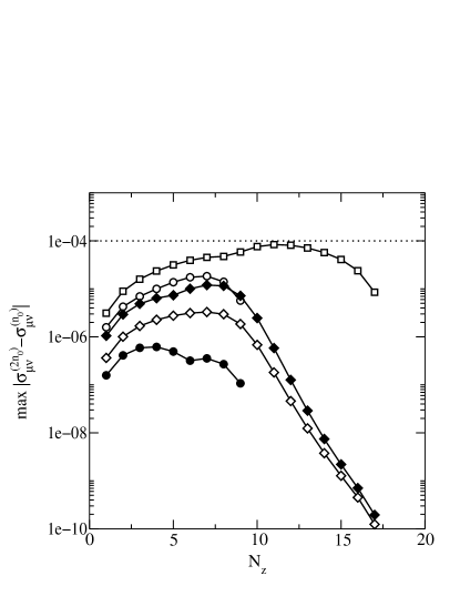
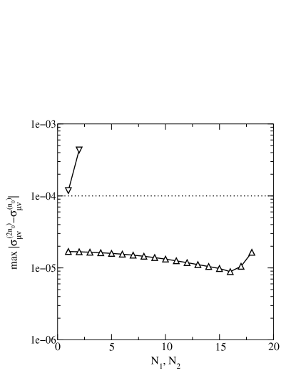
Figure 3: Maximum absolute difference between $\sigma_{\mu\nu}^{(2n_{0})}(\omega)$ and $\sigma_{\mu\nu}^{(n_{0})}(\omega)$ in atomic units for a complex energy points $N_{z}$ on a part of the contour or for a Matsubara pole $N_{1}$, $N_{2}$ ($n_{0}=8$, $\hbar\omega$ = 0.05 Ryd and $T$ = 300 K). Open (filled) symbols are used for the contour in the upper (lower) semi–plane. Circles refer to the quarter circles, squares to the parts parallel to the real axis and diamonds in the vicinity of the Fermi. $\vartriangle$ denotes the Matsubara poles far off from the real axis in the upper semi–plane and $\triangledown$ the others. The dotted line marks the value of $10^{-4}$ in atomic units.

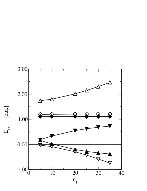
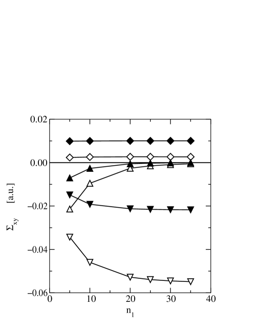
Figure 4: Real (open symbols) and imaginary part (filled symbols) of $\Sigma_{\mu\nu}(\omega)$, respectively, in atomic units for $\hbar\omega$ = 0.05 Ryd and $T$ = 300 K against the Matsubara poles $n_{1}$ in the upper semi–plane. (Triangles up are used for the contribution coming from the contour and triangles down for that coming from the Matsubara poles. Their sum is given by diamond. The convergence criteria (7) and (18) for $\varepsilon_{z}=\varepsilon_{\vec{k}}=10^{-4}$ a.u. were satisfied for each $n_{1}$ value considered.)

References

- [1] W. R. Bennett, W. Schwarzacher, and W. F. Egelhoff, Phys. Rev. Letters 65, 3169 (1990).
- [2] T. K. Hatwar, Y. S. Tyan, and C. F. Brucker, J. Appl. Physics 81, 3839 (1997).
- [3] Y. Suzuki, T. Katayama, P. B. S. Yuasa, and E. Tamura, Phys. Rev. Letters 80, 5200 (1998).
- [4] L. Szunyogh and P. Weinberger, J. Phys.: Condensed Matter 11, 10451 (1999).
- [5] J. M. Luttinger, in Mathematical Methods in Solid State and Superfluid Theory, edited by R. C. Clark and G. H. Derrick (Oliver and Boyd, Edingburgh, 1967), Chap. 4: Transport theory, p. 157.
- [6] C. S. Wang and J. Callaway, Phys. Rev. B 9, 4897 (1974).
- [7] P. Weinberger et al., J. Phys.: Condensed Matter 8, 7677 (1996).
- [8] R. Kubo, J. Phys. Soc. Japan 12, 570 (1957).
- [9] D. A. Greenwood, Proc. Phys. Soc. 71, 585 (1958).
- [10] W. H. Butler, Phys. Rev. B 31, 3260 (1985).
- [11] L. Szunyogh, B. Újfalussy, P. Weinberger, and J. Kollár, Phys. Rev. B 49, 2721 (1994).
- [12] L. Szunyogh, B. Újfalussy, and P. Weinberger, Phys. Rev. B 51, 9552 (1995).
- [13] B. Újfalussy, L. Szunyogh, and P. Weinberger, Phys. Rev. B 51, 12836 (1995).
- [14] W. H. Press, B. P. Flannery, S. A. Teukolsky, and W. T. Vetterling, Numerical recipes in Fortran: The art of scientific computing (Cambridge University Press, Cambridge, 1992).
- [15] Handbook of mathematical functions with formulas, graphs and mathematical tables, edited by M. Abramowitz and I. A. Stegun (Dover, New York, 1972).
- [16] A. S. Konrod, Nodes and weights of quadrature formulas (Consultants Bureau, New York, 1965).
- [17] D. Calvetti, G. H. Golub, W. B. Gragg, and L. Reichel, Math. Comput. 69, 1035 (2000).
- [18] D. P. Laurie, Math. Comput. 66, 1133 (1997).
-
[19]
W. Gautschi, ACM Trans. Math. Software 20, 21 (1994).
In particular, we used the RECUR routine to generate the recursion coefficients of a common set of orthogonal polynomials, e.g. Legendre polynomials, and the GAUSS routine to obtain the nodes and the weights of the –point Konrod rule and the weights of the associated –point Gauss rule, respectively. - [20] R. Piessens, QUADPACK: A subroutine package for automatic integration (Springer–Verlag, Berlin, 1983).
- [21] U. Pustogowa et al., Phys. Rev. B 60, 414 (1999).
- [22] J. Hama and M. Watanabe, J. Phys.: Condensed Matter 4, 4583 (1992).
- [23] L. Macot and B. Frank, Phys. Rev. B 41, 4469 (1990).
- [24] P. J. Lin-Chung, phys. stat. sol. (b) 85, 743 (1978).
- [25] M. J. Monkhorst and J. D. Pack, Phys. Rev. B 13, 5188 (1976).
- [26] D. J. Chadi and M. L. Cohen, Phys. Rev. B 8, 5747 (1973).
- [27] J. Moreno and J. M. Soler, Phys. Rev. B 45, 13 891 (1992).
- [28] S. L. Cunningham, Phys. Rev. B 10, 4988 (1974).
- [29] J. Hama, M. Watanabe, and T. Kato, J. Phys.: Condensed Matter 2, 7445 (1990).
- [30] –meshes, for example, with () are given in Ref. [29]. was applied to the three–dimensional hexagonal lattice in Ref. [22]. The frequently used, so–called Monkhorst–Pack meshes [25] are obtained considering . Particular two–dimensional Monkhorst–Pack meshes are given in Ref. [28].
- [31] As a corollary, it can be shown that a Monkhorst–Pack mesh cannot include all the –points of an other, similar Monkhorst–Pack mesh.
- [32] S. L. Altmann and P. Herzig, Point–Group Theory Tables (Clarendon Press, Oxford, 1994).
- [33] G. Hörmandinger and P. Weinberger, J. Phys.: Condensed Matter 4, 2185 (1992).