Evaluation of the optical conductivity tensor in terms of contour integrations

Abstract

For the case of finite life-time broadening the standard Kubo-formula for the optical conductivity tensor is rederived in terms of Green’s functions by using contour integrations, whereby finite temperatures are accounted for by using the Fermi-Dirac distribution function. For zero life-time broadening, the present formalism is related to expressions well-known in the literature. Numerical aspects of how to calculate the corresponding contour integrals are also outlined.

1 Introduction

A general theory of linear response functions has been formulated several decades ago [1], [2], [3] that became the basis of numerous studies of correlation functions, susceptibilities and transport properties in solid matter. Although early attempts were already devoted within this theoretical framework to magneto-optical phenomena, i.e., the Faraday and the Kerr effect, [4],[2] it was the rapid development of both, band structure methods and computational facilities that brought about the renaissance in this field from the end of the 1980’s (see [5], [6] and refs. therein). This progress was built on the assumption that the original expression for linear response functions, derived on the basis of a non-relativistic approach, is still valid when applying relativistic band structure methods. Recently, this has indeed been rigorously confirmed by Huhne and Ebert [7].

Within an independent particle picture the interband part of the optical conductivity tensor at finite temperatures, $\Sigma_{\mu\nu}(\omega)$ is given by [1], [3]

$$\Sigma_{\mu\nu}(\omega)=\frac{\hbar}{iV}\sum_{m,n}\frac{f(\epsilon_{n})(1\!-\!f(\epsilon_{m}))}{\epsilon_{n}\!-\!\epsilon_{m}}\left\{\frac{J_{nm}^{\mu}J_{mn}^{\nu}}{\hbar\omega+\epsilon_{n}-\epsilon_{m}+i\delta}+\frac{J_{nm}^{\nu}J_{mn}^{\mu}}{\hbar\omega+\epsilon_{m}-\epsilon_{n}+i\delta}\right\}\;,$$ (1)

where $\omega$ is the frequency, $f(\epsilon)$ is the Fermi function, $V$ is the volume of the system, the $J_{nm}^{\mu}=\langle n\!\mid\!J^{\mu}\!\mid\!m\rangle$ are the matrix elements of the current density operator $J^{\mu}$ ($\mu=x,y,z$) with respect to the eigenfunctions $\mid\!n\rangle$ of the one-electron Hamiltonian corresponding to energy eigenvalues $\epsilon_{n}$. Life-time broadening effects due to different scattering processes are partially accounted for by a finite value of $\delta=\hbar/\tau\sim 0.03$ Ry, where $\tau$ can be associated with a relaxation time [5, 6]. Such a life-time effect can naturally be incorporated into linear response theory either by assuming an adiabatic switch on of the external field $\phi({\bf r},t)=\phi({\bf r})e^{t/\tau}$ [8] or, equivalently, by convoluting the corresponding frequency dependent conductivity for $\delta\rightarrow+0$ by a Lorentzian of a finite halfwidth $\delta$.

Expression (1) is usually directly evaluated by applying standard band structure methods for ordered bulk (three-dimensional translational invariant) systems by associating the states $\mid n\rangle$ with (three-dimensional) Bloch-functions [2],[5]. This kind of approach, however, cannot be extended easily to layered systems or systems with a surface, i.e., to systems with (at best) two-dimensional translational symmetry. Furthermore, it is totally unsuited to deal with disorder such as interdiffusion effects in magnetic multilayer systems.

For zero life-time broadening an alternative approach consists of splitting Eq. (1) into an absorptive and a dispersive part, which in turn are interrelated via the Kramers-Kronig relations [4],[6]. Thus it is sufficient to directly calculate the absorptive part only, the corresponding Kubo-formula of which can be expressed in terms of Green’s functions as was shown by Butler [9] for $\omega=0$, and was used recently by Banhart [10] for $\omega>0$. Even much earlier, Luttinger [8] derived a general formula of the conductivity tensor which builts on the Green’s function of the system. However, when using this method the corresponding energy integrals have to be performed along the real axis which makes a calculation of $\Sigma_{\mu\nu}(\omega)$ enormously tedious and also numerically hard to control.

In the present work a suitable extension of Luttinger’s formula is given in terms of contour integrations that avoids the above mentioned numerical difficulties, is suitable for applications to magnetic multilayer systems and for treating alloying effects (interdiffusion etc.) by means of the Coherent Potential Approximation (CPA).

2 Contour integrations

Following Luttinger [8] Eq. (1) can be rewritten as

$$\Sigma_{\mu\nu}(\omega)=\frac{\sigma_{\mu\nu}(\zeta)\!-\!\sigma_{\mu\nu}(0)}{\zeta}\;,$$ (2)

where $\zeta=\omega+i\delta/\hbar$ and

$$\sigma_{\mu\nu}(\zeta)=\frac{i}{V}\sum_{m,n}\frac{f(\epsilon_{n})-f(\epsilon_{m})}{\hbar\zeta+\epsilon_{n}-\epsilon_{m}}J_{nm}^{\mu}J_{mn}^{\nu}\;.$$ (3)

For simplicity, as what follows, we denote $\sigma_{\mu\nu}(\zeta)$ by $\sigma_{\mu\nu}(\omega)$ [11] the calculation of which we will concentrate on keeping in mind that we have a finite imaginary part of the denominator in Eq. (3). Consider a pair of eigenvalues $\epsilon_{n}$ and $\epsilon_{m}$. For a suitable contour ${\cal{C}}$ in the complex energy plane (see Fig. 1) the residue theorem implies

$$\oint_{{\cal{C}}}\mbox{d}z\frac{f(z)}{(z-\epsilon_{n})(z-\epsilon_{m}+\hbar\omega+i\delta)} = -2\pi i\frac{f(\epsilon_{n})}{\epsilon_{n}-\epsilon_{m}+\hbar\omega+i\delta}\;+$$

$$+\;2i\delta_{T}\sum_{k=-N_{2}+1}^{N_{1}}\frac{1}{(z_{k}-\epsilon_{n})(z_{k}-\epsilon_{m}+\hbar\omega+i\delta)}\quad,$$

where the $z_{k}=\epsilon_{F}+i(2k-1)\delta_{T}$ ($\epsilon_{F}$ is the Fermi energy, $k_{B}$ the Boltzmann constant, $T$ the temperature and $\delta_{T}=\pi k_{B}T$) are the so-called Matsubara-poles. In Eq. (2) it was supposed that $N_{1}$ and $N_{2}$ Matsubara-poles in the upper and lower semi-plane lie within the contour ${\cal C}$, respectively, i.e.,

$$(2N_{1}-1)\delta_{T}<\delta_{1}<(2N_{1}+1)\delta_{T}\;,$$ (5)

$$(2N_{2}-1)\delta_{T}<\delta_{2}<(2N_{2}+1)\delta_{T}\;,$$ (6)

Eq. (2) can be rearranged as

$$i\frac{f(\epsilon_{n})}{\hbar\omega+\epsilon_{n}-\epsilon_{m}+i\delta}=-\frac{1}{2\pi}\oint_{{\cal{C}}}\mbox{d}z\frac{f(z)}{(z-\epsilon_{n})(z-\epsilon_{m}+\hbar\omega+i\delta)}\;+$$ (7)

$$+\;i\frac{\delta_{T}}{\pi}\sum_{k=-N_{2}+1}^{N_{1}}\frac{1}{(z_{k}-\epsilon_{n})(z_{k}-\epsilon_{m}+\hbar\omega+i\delta)}\quad.$$

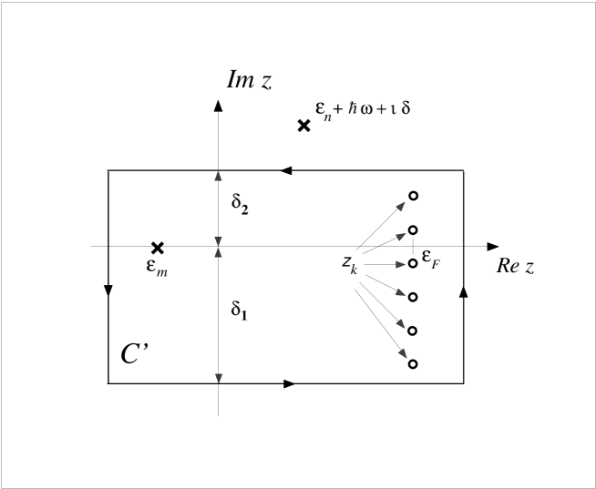
Figure 2: Contour in the complex plane corresponding to the integration in Eq. (8).

Similarly, by choosing a contour ${\cal{C}^{\prime}}$ as shown in Fig. 2 the following expression,

$$-i\frac{f(\epsilon_{m})}{\hbar\omega+\epsilon_{n}-\epsilon_{m}+i\delta}=\frac{1}{2\pi}\oint_{{\cal{C}^{\prime}}}\mbox{d}z\frac{f(z)}{(z-\epsilon_{m})(z-\epsilon_{n}-\hbar\omega-i\delta)}\;+$$ (8)

$$+\;i\frac{\delta_{T}}{\pi}\sum_{k=-N_{1}+1}^{N_{2}}\frac{1}{(z_{k}-\epsilon_{m})(z_{k}-\epsilon_{n}-\hbar\omega-i\delta)}$$

can be derived. Inserting Eqs. (7) and (8) into Eq. (3) and by closing the contours at $\infty$ and $-\infty$, $\sigma_{\mu\nu}(\omega)$ is given by

$$\sigma_{\mu\nu}(\omega)=-\frac{1}{2\pi V}\left\{\oint_{{\cal{C}}}\mbox{d}zf(z)\sum_{m,n}\frac{J_{nm}^{\mu}J_{mn}^{\nu}}{(z-\epsilon_{n})(z-\epsilon_{m}+\hbar\omega+i\delta)}\;-\right.$$ (9)

$$\left.\qquad\qquad\qquad\qquad\oint_{{\cal{C}^{\prime}}}\mbox{d}zf(z)\sum_{m,n}\frac{J_{nm}^{\mu}J_{mn}^{\nu}}{(z-\epsilon_{m})(z-\epsilon_{n}-\hbar\omega-i\delta)}\right\}$$

$$\qquad\qquad\;+\;i\frac{\delta_{T}}{\pi V}\left\{\sum_{k=-N_{2}+1}^{N_{1}}\;\sum_{m,n}\frac{J_{nm}^{\mu}J_{mn}^{\nu}}{(z_{k}-\epsilon_{n})(z_{k}-\epsilon_{m}+\hbar\omega+i\delta)}\;+\right.$$

$$\qquad\qquad\qquad\qquad\qquad\left.\sum_{k=-N_{1}+1}^{N_{2}}\;\sum_{m,n}\frac{J_{nm}^{\mu}J_{mn}^{\nu}}{(z_{k}-\epsilon_{m})(z_{k}-\epsilon_{n}-\hbar\omega-i\delta)}\right\}\quad.$$

It is now straightforward to rewrite Eq. (9) in terms of the resolvent [12],

$$G(z)=\sum_{n}\frac{\mid n\rangle\langle n\mid}{z-\epsilon_{n}}\;,$$ (10)

such that

$$\sigma_{\mu\nu}(\omega)=-\frac{1}{2\pi V}\left\{\oint_{{\cal{C}}}\mbox{d}zf(z)Tr\left[J^{\mu}G(z+\hbar\omega+i\delta)J^{\nu}G(z)\right]\;-\right.$$ (11)

$$\left.\qquad\qquad\qquad\quad\oint_{{\cal{C}^{\prime}}}\mbox{d}zf(z)Tr\left[J^{\mu}G(z)J^{\nu}G(z-\hbar\omega-i\delta)\right]\right\}$$

$$\qquad\qquad\;+\;i\frac{\delta_{T}}{\pi V}\left\{\sum_{k=-N_{2}+1}^{N_{1}}Tr\left[J^{\mu}G(z_{k}+\hbar\omega+i\delta)J^{\nu}G(z_{k})\right]\;+\right.$$

$$\qquad\qquad\qquad\qquad\;\;\left.\sum_{k=-N_{1}+1}^{N_{2}}Tr\left[J^{\mu}G(z_{k})J^{\nu}G(z_{k}-\hbar\omega-i\delta)\right]\right\}\;,$$

where $Tr$ denotes the trace of an operator. By using the below quantity, originally introduced by Butler [9],

$$\widetilde{\sigma}_{\mu\nu}(z_{1},z_{2})=-\frac{1}{2\pi V}Tr\left[J^{\mu}G(z_{1})J^{\nu}G(z_{2})\right]\;,$$ (12)

for which the following symmetry relations apply,

$$\widetilde{\sigma}_{\nu\mu}(z_{2},z_{1})=\widetilde{\sigma}_{\mu\nu}(z_{1},z_{2}),\quad\widetilde{\sigma}_{\mu\nu}(z_{1}^{*},z_{2}^{*})=\widetilde{\sigma}_{\nu\mu}(z_{1},z_{2})^{*}=\widetilde{\sigma}_{\mu\nu}(z_{2},z_{1})^{*},$$ (13)

$\sigma_{\mu\nu}(\omega)$ can be written as

$$\sigma_{\mu\nu}(\omega)=\oint_{{\cal{C}}}\mbox{d}zf(z)\widetilde{\sigma}_{\mu\nu}(z+\hbar\omega+i\delta,z)-\oint_{{\cal{C}^{\prime}}}\mbox{d}zf(z)\widetilde{\sigma}_{\mu\nu}(z,z-\hbar\omega-i\delta)$$ (14)

$$\qquad\qquad-2i\delta_{T}\left\{\sum_{k=-N_{2}+1}^{N_{1}}\widetilde{\sigma}_{\mu\nu}(z_{k}+\hbar\omega+i\delta,z_{k})+\sum_{k=-N_{1}+1}^{N_{2}}\widetilde{\sigma}_{\mu\nu}(z_{k},z_{k}-\hbar\omega-i\delta)\right\}\;,$$

which because of the reflection symmetry for the contours ${\cal C}$ and ${\cal C}^{\prime}$ (see Figs. 1 and 2) and the relations in Eq. (13) can be transformed to

$$\sigma_{\mu\nu}(\omega)=\oint_{{\cal{C}}}\mbox{d}zf(z)\widetilde{\sigma}_{\mu\nu}(z+\hbar\omega+i\delta,z)-\left(\oint_{{\cal{C}}}\mbox{d}zf(z)\widetilde{\sigma}_{\mu\nu}(z-\hbar\omega+i\delta,z)\right)^{*}$$ (15)

$$\qquad\qquad-2i\delta_{T}\sum_{k=-N_{2}+1}^{N_{1}}\left\{\widetilde{\sigma}_{\mu\nu}(z_{k}+\hbar\omega+i\delta,z_{k})+\widetilde{\sigma}_{\mu\nu}(z_{k}-\hbar\omega+i\delta,z_{k})^{*}\right\}\;.$$

Eq. (15) displays the central result of the present work: it compactly expresses the optical conductivity tensor in terms of contributions of a contour integral and those due to Matsubara poles. The occurring quantities of the type $\widetilde{\sigma}_{\mu\nu}(z_{1},z_{2})$ are now exactly of the form such that substitutional disorder (CPA) for layered systems [13, 14] can be treated. It should be noted that in the case of site-diagonal terms, see [14], in principle for the evaluation of the contour integrals also the ‘irregular’ part of the Green’s function has to be included. Since the inhomogeneous CPA for semi-infinite systems and the corresponding Kubo-Greenwood approach to electric transport is discussed at length in [14], no further discussion with respect to layered systems is needed.

3 Integration along the real axis: the limit of zero life-time broadening

In this Section we give the relationship of Eq. (15) to formulations existing in the literature. For this reason the contour ${\cal C}$ is deformed to the real axis such that the contributions from the Matsubara poles vanish. By using the relations in Eq. (13) Eq. (15) reduces to

$$\sigma_{\mu\nu}(\omega) = \int_{-\infty}^{\infty}\mbox{d}\epsilon f(\epsilon)\;[\widetilde{\sigma}_{\mu\nu}(\epsilon+\hbar\omega+i\delta,\epsilon+i0)-\widetilde{\sigma}_{\mu\nu}(\epsilon+\hbar\omega+i\delta,\epsilon\!-\!i0)]$$

$$- \int_{-\infty}^{\infty}\mbox{d}\epsilon f(\epsilon)\>[\widetilde{\sigma}_{\mu\nu}(\epsilon\!-\!i0,\epsilon\!-\!\hbar\omega\!-\!i\delta)\!-\!\widetilde{\sigma}_{\mu\nu}(\epsilon+i0,\epsilon\!-\!\hbar\omega\!-\!i\delta)]$$

$$=-\frac{1}{2\pi V}\int_{-\infty}^{\infty}\mbox{d}\epsilon f(\epsilon)Tr\left\{J^{\mu}G(\epsilon+\hbar\omega+i\delta)J^{\nu}\{G^{+}(\epsilon)\!-\!G^{-}(\epsilon)\}\right.$$ (17)

$$\left.\qquad\qquad\qquad\qquad\qquad+J^{\mu}\{G^{+}(\epsilon)\!-\!G^{-}(\epsilon)\}J^{\nu}G(\epsilon\!-\!\hbar\omega\!-\!i\delta)\right\}\;,$$

where we introduced up- and down-side limits for the resolvents [12]. By taking the limit $\delta\rightarrow 0$ Eq. (17) becomes equivalent to Eq. (5.15) of Ref. [8] for q=0,

$$\sigma_{\mu\nu}(\omega)=-\frac{1}{2\pi V}\int_{-\infty}^{\infty}\mbox{d}\epsilon f(\epsilon)Tr\left\{J^{\mu}G^{+}(\epsilon+\hbar\omega)J^{\nu}\{G^{+}(\epsilon)\!-\!G^{-}(\epsilon)\}\right.$$ (18)

$$\left.\qquad\qquad\qquad\qquad\qquad\qquad\qquad+J^{\mu}\{G^{+}(\epsilon)\!-\!G^{-}(\epsilon)\}J^{\nu}G^{-}(\epsilon\!-\!\hbar\omega)\right\}\;.$$

Note that by shifting in the second term of Eq. (18) the argument of integration by $\hbar\omega$ the hermitean part of $\sigma_{\mu\nu}(\omega)$ can be expressed as

$$\sigma_{1,\mu\nu}(\omega)\equiv\frac{1}{2}(\sigma_{\mu\nu}(\omega)+\sigma_{\nu\mu}(\omega)^{*})=-\frac{1}{4\pi V}\int_{-\infty}^{\infty}\mbox{d}\epsilon\;(f(\epsilon)-f(\epsilon+\hbar\omega))\times\qquad\qquad\qquad\qquad$$ (19)

$$\qquad\qquad\qquad\qquad\qquad\qquad\qquad\qquad Tr\left\{J^{\mu}\{G^{+}(\epsilon+\hbar\omega)\!-\!G^{-}(\epsilon+\hbar\omega)\}J^{\nu}\{G^{+}(\epsilon)\!-\!G^{-}(\epsilon)\}\right\}\;.$$

Since quite clearly $\sigma_{1,\mu\nu}(0)=0$, from Eq. (2) we get $\Sigma_{1,\mu\nu}(\omega)=\sigma_{1,\mu\nu}(\omega)/\omega$ as used in Ref. [10].

In order to obtain the correct zero frequency formula one has to take first the $\omega\rightarrow 0$ limit of Eq. (3) and then, after inserting into Eq. (2), the $\delta\rightarrow 0$ limit has to be performed. Making use of the analyticity of the Green’s functions in the upper and lower complex semi-planes this leads to [16]

$$\Sigma_{\mu\nu}(0)=-\frac{\hbar}{2\pi V}\int_{-\infty}^{\infty}\mbox{d}\epsilon\>f(\epsilon)\;Tr\left\{J^{\mu}\frac{\partial G^{+}(\epsilon)}{\partial\epsilon}J^{\nu}[G^{+}(\epsilon)\!-\!G^{-}(\epsilon)]-J^{\mu}[G^{+}(\epsilon)\!-\!G^{-}(\epsilon)]J^{\mu}\frac{\partial G^{-}(\epsilon)}{\partial\epsilon}\right\}\;,$$ (20)

which can be integrated by parts. The corresponding expression at $T=0$ for the diagonal elements yields Butler’s original formula [9],

$$\Sigma_{\mu\mu}(0)_{(T=0)}=-\frac{\hbar}{4\pi V}Tr\left\{J^{\mu}[G^{+}(\epsilon_{F})\!-\!G^{-}(\epsilon_{F})]J^{\mu}[G^{+}(\epsilon_{F})\!-\!G^{-}(\epsilon_{F})]\right\}\;.$$ (21)

4 Practical evaluation of the contour integrals

Returning to Eq. (15) we are left with the task to evaluate the occurring contour integrals in a manner suitable for computational purposes. This is in particular demanding because, in principle, integrations from $-\infty$ to $\infty$ are involved. Recalling Fig. 1, it is essential to note that the integration pathes can be chosen arbitrarily with the only constraint that the one in the lower complex semi-plane should lie in the range $0>Im(z)>-\delta$. It is trivial to show that, if the contributions from the core-states are not considered, the contour ${\cal C}$ can be closed at $\epsilon_{b}$ (bottom of the valence band) which lies energetically just below the regime of valence states. Consequently, the integrals in Eq. (15) can be split up as follows

$$\oint_{{\cal{C}}}\mbox{d}zf(z)\widetilde{\sigma}_{\mu\nu}(z\pm\hbar\omega+i\delta,z)=$$ (22)

$$\int_{\epsilon_{b}+i0}^{\infty+i\delta_{1}}\mbox{d}zf(z)\widetilde{\sigma}_{\mu\nu}(z\pm\hbar\omega+i\delta,z)-\int_{\epsilon_{b}\!-\!i0}^{\infty\!-\!i\delta_{2}}\mbox{d}zf(z)\widetilde{\sigma}_{\mu\nu}(z\pm\hbar\omega+i\delta,z)\;.$$

Because of the fast decay of the Fermi function $f(z)$ for $Re(z)>\epsilon_{F}$ the integrals on the $rhs$ of Eq. (22) can be terminated at

$$\epsilon_{u}=\epsilon_{F}+n\,k_{B}T\qquad(n\simeq 5-10).$$

Finally, after manipulating the contributions from the Matsubara poles, see Eq. (15), the optical conductivity (or rather the zero wave-number current-current correlation function [11]) can be written as

$$\sigma_{\mu\nu}(\omega)=\sigma^{1}_{\mu\nu}(\omega)+\sigma^{2}_{\mu\nu}(\omega)+\sigma^{3}_{\mu\nu}(\omega)\;,$$ (23)

where

$$\sigma_{\mu\nu}^{1}(\omega)=\int_{\epsilon_{b}+i0}^{\epsilon_{u}+i\delta_{1}}\mbox{d}zf(z)\widetilde{\sigma}_{\mu\nu}(z+\hbar\omega+i\delta,z)-\left(\int_{\epsilon_{b}+i0}^{\epsilon_{u}+i\delta_{1}}\mbox{d}zf(z)\widetilde{\sigma}_{\mu\nu}(z-\hbar\omega+i\delta,z)\right)^{*}\;,$$ (24)

$$\sigma_{\mu\nu}^{2}(\omega)=-\int_{\epsilon_{b}-i0}^{\epsilon_{u}-i\delta_{2}}\mbox{d}zf(z)\widetilde{\sigma}_{\mu\nu}(z+\hbar\omega+i\delta,z)+\left(\int_{\epsilon_{b}-i0}^{\epsilon_{u}-i\delta_{2}}\mbox{d}zf(z)\widetilde{\sigma}_{\mu\nu}(z-\hbar\omega+i\delta,z)\right)^{*}\;,$$ (25)

and

$$\sigma_{\mu\nu}^{3}(\omega)=\!\! -\!\! \!\!2i\delta_{T}\sum_{k=N_{2}+1}^{N_{1}}\{\widetilde{\sigma}_{\mu\nu}(\epsilon_{F}+\hbar\omega+i[\delta+(2k-1)\delta_{T}],\epsilon_{F}+i(2k-1)\delta_{T})$$

$$\qquad\qquad\left.+\,\widetilde{\sigma}_{\mu\nu}(\epsilon_{F}-\hbar\omega+i[\delta+(2k-1)\delta_{T}],\epsilon_{F}+i(2k-1)\delta_{T})^{*}]\right\}$$

$$-\!\! \!\!2i\delta_{T}\;\;\sum_{k=1}^{N_{2}}\;\left\{\widetilde{\sigma}_{\mu\nu}(\epsilon_{F}+\hbar\omega+i[\delta+(2k-1)\delta_{T}],\epsilon_{F}+i(2k-1)\delta_{T})\right.$$

$$\qquad\quad\;\;+\widetilde{\sigma}_{\mu\nu}(\epsilon_{F}-\hbar\omega+i[\delta+(2k-1)\delta_{T}],\epsilon_{F}+i(2k-1)\delta_{T})^{*}$$

$$\qquad\quad\;\;+\widetilde{\sigma}_{\mu\nu}(\epsilon_{F}+\hbar\omega+i[\delta-(2k-1)\delta_{T}],\epsilon_{F}-i(2k-1)\delta_{T})$$

$$\qquad\quad\;\;+\left.\!\!\widetilde{\sigma}_{\mu\nu}(\epsilon_{F}-\hbar\omega+i[\delta-(2k-1)\delta_{T}],\epsilon_{F}-i(2k-1)\delta_{T})^{*}\right\}\;.$$

Preliminary calculations show that by choosing $\delta\simeq 0.05$ Ryd, $\delta_{1}\simeq 0.1-0.15$ Ryd and by using Gaussian-quadrature a total of 30 - 100 energy points (depending on $\hbar\omega$) is sufficient to sample the above energy integrals. Furthermore, since most of these energy points lie either below the valence band or far enough away from the real axis (the energy point closest to the real axis is at $z_{1}=\epsilon_{F}+i\delta_{T}$, where for $T=300$ K $\delta_{T}\simeq 6$ mRyd), the occurring Brillouin-zone integrals (see Ref. [14]) can be evaluated by using a sufficiently small set of ${\bf k}$-points in the surface Brillouin zone, thus ensuring excellent numerical stability.

5 Summary

In the present paper, by using a finite life-time broadening (or a finite adiabatic switch-on parameter) we reformulated the expression for the (linear response) optical conductivity tensor in terms of contour integrations such that Green’s functions (resolvents) naturally appear and finite temperatures are represented by the Fermi-Dirac distribution function. For zero life-time broadening the traditional expressions of the conductivity tensor in terms of the Green’s function are recovered. Finally, a scheme for calculating the contour integrals that occur, in a numerically efficient way, is suggested. Although primarily applications to ab-initio calculations of magneto-optical properties of ordered and disordered thin films in terms of the fully-relativistic spin-polarized Screened Korringa-Kohn-Rostoker method [14, 15] are currently under way, it should be noted that the present method can also be used to calculate other linear response functions, just as readily as it can easily be extended to the evaluation of non-linear response functions.

Acknowledgements

The authors are especially grateful to Prof. B.L. Györffy for many stimulating discussions. This paper resulted from a collaboration partially funded by the Research and Technological Cooperation between Austria and Hungary (OMFB-Bundesministerium für Auswärtige Angelegenheiten, Contract No. A-35/98). Financial support was provided also by the Austrian Science Foundation (Contract No.’s P12146 and P12352), and the Hungarian National Science Foundation (Contract No.’s OTKA T024137 and T030240).

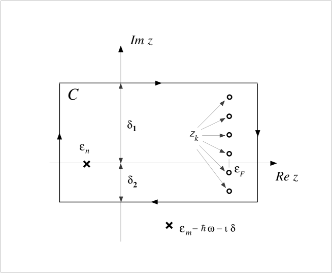
Figure 1: Contour in the complex plane corresponding to the integration in Eq. (2).

References

- [1] R. Kubo, J. Phys. Soc. Jpn. 12, 570 (1957).
- [2] C.S. Wang and J. Callaway, Phys. Rev. B 9, 4897 (1974).
- [3] J. Callaway, Quantum Theory of the Solid State, part B (New York: Academic, 1974).
- [4] H.S. Bennett and E.A. Stern, Phys. Rev. 137, A448 (1965).
- [5] P. M. Oppeneer and V. N. Antonov, In: Spin-orbit-influenced Spectroscopies of Magnetic Solids, p. 29 - 47, (Eds.: H. Ebert and G. Schütz), Springer Verlag 1996.
- [6] H. Ebert, Rep. Prog. Phys. 59, 1665 (1996).
- [7] T. Huhne and H. Ebert, submitted to Phys. Rev. B (1999). In there it is claimed that in a fully relativistic formalism the so-called diamagnetic contribution to the conductivity is not explicitely present.
- [8] J.M. Luttinger, in Mathematical Methods in Solid State and Superfluid Theory, Eds. R.C.Clark and G.H.Derrick (Oliver & Boyd, Edinburgh, 1967) pp. 157-193.
- [9] W. H. Butler, Phys. Rev. B 31, 3260 (1985).
- [10] J. Banhart, Phys. Rev. Lett. 82, 2139 (1999).
- [11] In fact , where is the current-current correlation function. Compare with Eq. (3.8.9) of G.D. Mahan, Many-Particle Physics, Plenum Press, New York, 1990.
- [12] P. Weinberger, Electron Scattering for Ordered and Disordered Matter, Clarendon Press, 1990.
- [13] W. H. Butler, X.-G. Zhang and D.M.C. Nicholson, J. Appl. Phys. 76, 6808 (1994); W.H. Butler, X.-G. Zhang, D.M.C. Nicholson and J.M. MacLaren, Phys. Rev. B 52, 13399 (1995).
- [14] P. Weinberger, P.M. Levy, J. Banhart, L. Szunyogh, and B. Újfalussy, J. Phys.: Condens. Matter 8, 7679 (1996).
- [15] L. Szunyogh, B. Újfalussy, and P. Weinberger, Phys. Rev. B 51, 9552 (1995).
- [16] L. Smrčka and P. Středa, J. Phys. C 10, 2153 (1977).