LAYER–RESOLVED MAGNETO–OPTICAL KERR EFFECT IN SEMI–INFINITE INHOMOGENEOUS LAYERED SYSTEMS

Abstract

The contour integration technique applied to calculate the optical conductivity tensor at finite temperatures in the case of inhomogeneous surface layered systems within the framework of the spin–polarized relativistic screened Korringa–Kohn–Rostoker band structure method is extended to arbitrary polarizations of the electric field. It is shown that besides the inter–band contribution, the contour integration technique also accounts for the intra-band contribution too. Introducing a layer–resolved complex Kerr angle, the importance of the first, non–magnetic buffer layer below the ferromagnetic surface on the magneto–optical Kerr effect in the $\mathrm{Co}\mid\mathrm{Pt}_{m}$ multilayer system is shown. Increasing the thickness of the buffer Pt, the layer–resolved complex Kerr angles follow a linear dependence with respect to $m$ only after nine Pt mono–layers.

1 Introduction

The magneto–optical Kerr effect (MOKE) was discovered by Rev. J. Kerr in 1876. Nowadays, the MOKE occurring in multilayers is investigated because of obvious technological implications for high–density magneto–optic recording media Bertero and Sinclair (1994); Mansuripur (1995).

The first ab–initio calculation of the absorptive part of the optical conductivity tensor based on the Kubo linear response theory Kubo (1957), was carried out for Ni by Wang and Callaway (1974). The dispersive part of the optical conductivity tensor, needed to get the theoretical MOKE, is usually computed using the Kramers–Kronig relations Daalderop et al. (1988). However, the first magneto–optical Kerr spectra, namely those for Fe and Ni, were calculated on the basis of a relativistic band–structure method by Oppeneer et al. (1992).

Commonly, the MOKE calculations for multilayers are performed using conventional band–structure methods and super–cells Guo and Ebert (1995); Uba et al. (1996). The contour integration technique developed by two of the authors Szunyogh and Weinberger (1999) used in connection with the spin–polarized relativistic screened Korringa–Kohn–Rostoker (SKKR) method Szunyogh et al. (1994, 1995); Újfalussy et al. (1995), on the other hand, is a more realistic approach for the magneto–optical Kerr spectra calculations in case of surface layered systems.

In the next section (Section 2) the theoretical framework is revisited and extended to arbitrary polarizations of the electric field. In Section 2.2 it is demonstrated that besides the inter–band contribution to the optical conductivity tensor, the contour integration technique Szunyogh and Weinberger (1999) includes also the intra–band contribution. In Section 2.3 it is shown that the Luttinger formalism Luttinger (1967) – and accordingly the contour integration technique too – provides the complex conductivity tensor even in the zero frequency limit for a finite life–time broadening. The symmetric part of the dc conductivity tensor, however, cannot be obtained by contour integrating in the complex energy plane. Recently, the authors discussed in details schemes of how to control the accuracy of the computation Vernes et al. (2000), therefore in Section 3 only the main aspects of these numerical methods are briefly reviewed. In Section 4 the layer–resolved complex Kerr angles are introduced. This concept is then used to study separately the impact of the ferromagnetic surface layer and of the non–magnetic buffer layers below the surface in the $\mathrm{Co}\mid\mathrm{Pt}_{m}$ surface layered system. In addition, the change of MOKE with the thickness of the buffer Pt–layer for a particular frequency is also analyzed. Finally, the main results of the present work are summarized in Section 5.

2 Theoretical framework

When a time dependent external electric field is applied to a solid, currents are induced, which create internal electric fields. The total electric field is then the sum of all these fields and in the long–wavelength limit is written as Eykholt (1986)

$$\vec{E}(\vec{r},t)=\vec{E}_{0}\ e^{i(\vec{q}\,\vec{r}-\omega t)}\ e^{\delta t}\ ,$$ (1)

the positive infinitesimal $\delta$ implying the field to be turned on at $t=-\infty$ Lax (1958).

Because the solid is not a homogeneous system, in linear response the resulting total current density is given by Mahan (1990)

$$J_{\mu}(\vec{r},t)=\sum_{\nu}\int d^{3}r^{\prime}\int dt^{\prime}\ \Sigma_{\mu\nu}(\vec{r},\vec{r}^{\,\prime};t,t^{\prime})E_{\nu}(\vec{r}^{\,\prime},t^{\prime})\ .$$ (2)

Here $\Sigma_{\mu\nu}(\vec{r},\vec{r}^{\,\prime};t,t^{\prime})$ is the non–local, time dependent conductivity and expresses the linear response of the current at $t$ in $\vec{r}$ and direction $\mu$ to the local electric field applied at $t^{\prime}$ in $\vec{r}^{\,\prime}$ and direction $\nu$ Butler et al. (1994).

The Fourier transform of Eq. (2)

$$J_{\mu}(\vec{q}^{\,\prime},\omega^{\prime})=\delta_{\vec{q}^{\,\prime},\vec{q}}\delta(\omega^{\prime}-\omega)\sum_{\nu}\Sigma_{\mu\nu}(\vec{q},\omega)E_{0\nu}\qquad(\mu,\nu=\mathrm{x,y,z})\ ,$$

introduces the wave–vector and frequency dependent complex conductivity tensor $\boldsymbol{\Sigma}(\vec{q},\omega)$ Eykholt (1986), which can be evaluated using the well–known Kubo formula Kubo (1957)

$$\Sigma_{\mu\nu}(\vec{q},\omega)=\lim_{\delta\rightarrow 0^{+}}\frac{1}{V}\int_{0}^{\infty}dt\ e^{\frac{i}{\hbar}\left(\hbar\omega+i\delta\right)t}\int_{0}^{\beta}d\lambda\ \left\langle J_{-\vec{q}}^{\nu}\ J_{\vec{q}}^{\mu}\left(t+i\hbar\lambda\right)\right\rangle_{\mathrm{eq}}\ .$$ (3)

Here $V$ is the crystalline volume, $\beta=\left(k_{\mathrm{B}}T\right)^{-1}$ and $\langle\ldots\rangle_{\mathrm{eq}}$ the ensemble average in the equilibrium state at $t=-\infty$, respectively. Notice that when the electric field is not transverse, i.e. $\vec{q}\vec{E}_{0}\neq 0$ Eykholt (1986); Mahan (1990), the Kubo conductivity tensor $\boldsymbol{\Sigma}(\vec{q},\omega)$ differs from that derived from the Maxwell equations Kubo (1966), i.e.

$$\boldsymbol{\Sigma}_{\mathrm{M}}(\vec{q},\omega)=\boldsymbol{\Sigma}(\vec{q},\omega)\left[1-\dfrac{4\pi i}{\omega}\ \hat{q}\cdot\boldsymbol{\Sigma}(\vec{q},\omega)\cdot\hat{q}\right]^{-1}\ ,$$

where $\hat{q}$ is the unit vector along $\vec{q}$.

2.1 Luttinger formalism

Based on the contour deformation method Yu-Kuang Hu (1993), it can be easily shown that

$$\int_{0}^{\beta}d\lambda\ \left\langle J_{-\vec{q}}^{\nu}\ J_{\vec{q}}^{\mu}\left(t+i\hbar\lambda\right)\right\rangle_{\mathrm{eq}}=\frac{i}{\hbar}\int_{t}^{\infty}dt^{\prime}\ \left\langle\left[J_{\vec{q}}^{\mu}\left(t^{\prime}\right),\ J_{-\vec{q}}^{\nu}\right]\right\rangle_{\mathrm{eq}}\ ,$$

where $J_{\vec{q}}^{\mu}\left(t^{\prime}\right)$ is the Heisenberg operator:

$$J_{\vec{q}}^{\mu}\left(t^{\prime}\right)=e^{\frac{i}{\hbar}Ht^{\prime}}\ J_{\vec{q}}^{\mu}\ e^{-\frac{i}{\hbar}Ht^{\prime}}\ .$$

For a diagonal representation of the one–electron Hamiltonian $H$ and for the equilibrium density operator

$$\rho_{\mathrm{eq}}\equiv f(H)=\dfrac{1}{e^{\beta(H-\mu)}+1}\ ,$$

with $f(H)$ being the Fermi–Dirac distribution function, $\mu$ the chemical potential (in the following the temperature dependence of the chemical potential is neglected, i.e. $\mu$ equals the Fermi level $\varepsilon_{\mathrm{F}}$), Eq. (3) can be rewritten as

$$\Sigma_{\mu\nu}(\vec{q},\omega) =\lim_{\delta\rightarrow 0^{+}}\frac{i}{\hbar V}\sum_{m,n}\ \left[f(\varepsilon_{m})-f(\varepsilon_{n})\right]\ J_{\vec{q},mn}^{\mu}\ J_{-\vec{q},nm}^{\nu}$$ (4)

$$\cdot\int_{0}^{\infty}dt\ e^{\frac{i}{\hbar}\left(\hbar\omega+i\delta\right)t}\int_{t}^{\infty}dt^{\prime}\ e^{\frac{i}{\hbar}(\varepsilon_{m}-\varepsilon_{n})t^{\prime}}\ ,$$

where

$$J_{\vec{q},mn}^{\mu}\equiv\left\langle m\right|J_{\vec{q}}^{\mu}\left|n\right\rangle\ ,\quad J_{-\vec{q},nm}^{\nu}\equiv\left\langle n\right|J_{-\vec{q}}^{\nu}\left|m\right\rangle\ ,$$

and $\varepsilon_{m}$ denotes the eigenvalue of $H$ corresponding to the eigenvector $\left|m\right\rangle$.

Both integrations in Eq. (4) with respect to $t^{\prime}$ and $t$, respectively, can be performed taking advantage on the Laplace transform of the identity Abramowitz and Stegun (1972). Proceeding by this manner, the factor $e^{\delta t}$ introduced in Eq. (1) to describe the interaction of the solid with its surroundings, can be seen also as a simple convergence factor Lax (1958). However, the complex conductivity tensor a for finite $\zeta=\hbar\omega+i\delta$, i.e.

$$\Sigma_{\mu\nu}(\vec{q},\zeta)=\frac{\hbar}{iV}\sum_{m,n}\ \frac{f(\varepsilon_{m})-f(\varepsilon_{n})}{\varepsilon_{m}-\varepsilon_{n}}\ \frac{J_{\vec{q},mn}^{\mu}\ J_{-\vec{q},nm}^{\nu}}{\varepsilon_{m}-\varepsilon_{n}+\zeta}\ ,$$ (5)

extends further the meaning of $\delta$. Here, $\delta$ can be seen as the finite life–time broadening, which accounts for all the scattering processes at finite temperature, which are not part of a standard band–structure calculation. Introducing the current–current correlation function as Mahan (1990)

$$\sigma_{\mu\nu}\left(\vec{q},\zeta\right)=\frac{i\hbar}{V}\sum_{m,n}\ \frac{f(\varepsilon_{m})-f(\varepsilon_{n})}{\varepsilon_{m}-\varepsilon_{n}+\zeta}\ J_{\vec{q},mn}^{\mu}\ J_{-\vec{q},nm}^{\nu}\quad,$$ (6)

finally results the well–known Luttinger formula Luttinger (1967)

$$\Sigma_{\mu\nu}(\vec{q},\zeta)=\frac{\sigma_{\mu\nu}\left(\vec{q},\zeta\right)-\sigma_{\mu\nu}\left(\vec{q},0\right)}{\zeta}\quad.$$ (7)

A rather technical point to be noticed is that in a previous paper Szunyogh and Weinberger (1999), the variable $\zeta$ has a slightly different definition, namely it was introduced as short–hand notation for $\omega+i\delta/\hbar$. For this meaning of $\zeta$, one has to use Eqs. (2) and (3) from Szunyogh and Weinberger (1999) instead of Eqs. (6) and (7).

The Luttinger formula (7) differs in form from that originally deduced by Kubo using the scalar potential description of the electric field Kubo (1957). In fact, Eq. (6) can be straightforwardly obtained starting from the vector potential description of the electric field Callaway (1974). Nevertheless, the formulae arising from the different descriptions of the electric field are completely equivalent Yu-Kuang Hu (1993).

The inter–band contribution to the complex conductivity tensor $\Sigma_{\mu\nu}^{\mathrm{inter}}(\vec{q},\zeta)$, can be obtained directly from Eqs. (6) and (7), imposing for the former $\varepsilon_{m}\neq\varepsilon_{n}$. Considering the intra–band life–time broadening equal to that taken for the inter–band contribution, Eq. (5) provides in the $\varepsilon_{m}\rightarrow\varepsilon_{n}$ limit immediately the intra–band contribution

$$\Sigma_{\mu\nu}^{\mathrm{intra}}(\vec{q},\zeta)=\dfrac{\sigma_{\mu\nu}^{\mathrm{intra}}(\vec{q})}{\zeta}\ ,$$ (8)

where

$$\sigma_{\mu\nu}^{\mathrm{intra}}(\vec{q})\equiv-\lim_{\varepsilon_{m}\rightarrow\varepsilon_{n}}\sigma_{\mu\nu}(\vec{q},0)\ ,$$ (9)

because $\sigma_{\mu\nu}^{\mathrm{intra}}\left(\vec{q},\zeta\right)=0$, if $\zeta\neq 0$. In contrast to the phenomenological Drude term, which is supposed to give the intra–band contribution Oppeneer et al. (1992), $\Sigma_{\mu\nu}^{\mathrm{intra}}(\vec{q},\zeta)$ is added to both, diagonal ($\mu=\nu$) and off–diagonal ($\mu\neq\nu$) elements of the complex conductivity tensor Oppeneer (1999). In conclusion, calculating $\sigma_{\mu\nu}\left(\vec{q},\zeta\right)$ in accordance with Eq. (6), both the inter– and intra–band contribution is present in the Luttinger formula (7), i.e.

$$\Sigma_{\mu\nu}(\vec{q},\zeta)=\Sigma_{\mu\nu}^{\mathrm{inter}}(\vec{q},\zeta)+\Sigma_{\mu\nu}^{\mathrm{intra}}(\vec{q},\zeta)\ .$$

2.2 Contour integration technique

The contour integration technique, originally developed for $\vec{q}=0$ by Szunyogh and Weinberger (1999), is extended below to calculate the current–current correlation function for arbitrary polarizations of the electric field. This technique permits the evaluation of Eq. (6) by performing a contour integration in the complex energy plane at finite temperature. The integration can be performed by exploiting the properties of the Fermi–Dirac distribution in the selection of the contour Mahan (1990),

$$f(z)=\frac{1}{e^{\beta(z-\mu)}+1}\quad\ ,$$

with $z\in\mathbb{C}$. Namely, that $f(z)$ is analytical everywhere, except the so–called Matsubara poles Nicholson et al. (1994)

$$z_{k}=\varepsilon_{\mathrm{F}}+i\left(2k-1\right)\delta_{T}\ ,\qquad k=0,\pm 1,\pm 2,\ldots$$

($\delta_{T}=\pi k_{\mathrm{B}}T$) and for energies parallel to the real axis situated in–between two, successive Matsubara poles Wildberger et al. (1995), $f(\varepsilon\pm 2ik\delta_{T})=f(\varepsilon)$.

Initially, two contours $\Gamma_{1}$ and $\Gamma_{2}$ are considered around the eigenvalues $\varepsilon_{m}$ and $\varepsilon_{n}$ including a finite number of Matsubara poles, see Fig. 1. The contour parts of $\Gamma_{1}$ parallel to the real axis ($z=\varepsilon\pm i\delta_{j}$, $j=1,2$) are taken in–between two, successive Matsubara poles

$$(2N_{j}-1)\delta_{T}<\delta_{j}<(2N_{j}+1)\delta_{T}\ ,$$ (10)

with $N_{1}$ being the Matsubara poles in the upper and $N_{2}$ in the lower semi–plane, respectively, included in $\Gamma_{1}$, e.g. $\delta_{j}=2N_{j}\delta_{T}$ for $j=1,2$. $\Gamma_{2}$ is $\Gamma_{1}$ mirrored along the real axis, hence includes $N_{2}$ Matsubara poles in the upper and $N_{1}$ in the lower semi–plane. In order to not have $\varepsilon_{n}-\zeta$ and $\varepsilon_{m}+\zeta$ contained in the contour $\Gamma_{2}$ and $\Gamma_{1}$, respectively, the only constraint applied is

$$\delta>\delta_{2}\ .$$ (11)

Using the residue theorem, it was shown that Szunyogh and Weinberger (1999)

$$i\frac{f(\varepsilon_{m})}{\varepsilon_{m}-\varepsilon_{n}+\zeta}= -\frac{1}{2\pi}\int_{\Gamma_{1}}\circlearrowright\ dz\frac{f(z)}{\left(z-\varepsilon_{m})(z-\varepsilon_{n}+\zeta\right)}$$

$$+i\frac{\delta_{T}}{\pi}\sum_{k=-N_{2}+1}^{N_{1}}\frac{1}{(z_{k}-\varepsilon_{m})(z_{k}-\varepsilon_{n}+\zeta)}$$

and

$$-i\frac{f(\varepsilon_{n})}{\varepsilon_{m}-\varepsilon_{n}+\zeta} =\frac{1}{2\pi}\int_{\Gamma_{2}}\circlearrowleft\ dz\frac{f(z)}{\left(z-\varepsilon_{n}\right)\left(z-\varepsilon_{m}-\zeta\right)}$$

$$+i\frac{\delta_{T}}{\pi}\sum_{k=-N_{1}+1}^{N_{2}}\frac{1}{(z_{k}-\varepsilon_{n})(z_{k}-\varepsilon_{m}-\zeta)}\ .$$

Observing that as long as $\zeta\neq 0$, the sum of these two expressions vanishes, when $\varepsilon_{m}=\varepsilon_{n}$, no restriction regarding to the eigenvalues must be imposed, such that by using the resolvent Weinberger (1990)

$$G(z)=\sum_{n}\frac{\left|n\rangle\langle n\right|}{z-\varepsilon_{n}}\ ,$$

immediately follows that

$$\sigma_{\mu\nu}(\vec{q},\zeta) =\int_{\Gamma_{1}}\circlearrowright\ dz\ f(z)\ \tilde{\sigma}_{\mu\nu}(\vec{q};z+\zeta,z)-\int_{\Gamma_{2}}\circlearrowleft\ dz\ f(z)\ \tilde{\sigma}_{\mu\nu}(\vec{q};z,z-\zeta)$$

$$-2i\delta_{T}\left[\sum_{k=-N_{2}+1}^{N_{1}}\tilde{\sigma}_{\mu\nu}(\vec{q};z_{k}+\zeta,z_{k})+\sum_{k=-N_{1}+1}^{N_{2}}\tilde{\sigma}_{\mu\nu}(\vec{q};z_{k},z_{k}-\zeta)\right]\ .$$ (12)

Here due to the trace, the quantity

$$\tilde{\sigma}_{\mu\nu}(\vec{q};z_{1},z_{2})=-\frac{\hbar}{2\pi V}\ \mathrm{Tr}\left[J_{\vec{q}}^{\mu}\ G(z_{1})\ J_{-\vec{q}}^{\nu}\ G(z_{2})\right]\ ,$$ (13)

contains the inter–band ($\varepsilon_{m}\neq\varepsilon_{n}$) and the vanishing intra–band ($\varepsilon_{m}=\varepsilon_{n}$) contribution too, i.e.

$$\sigma_{\mu\nu}(\vec{q},\zeta)=\sigma_{\mu\nu}^{\mathrm{inter}}(\vec{q},\zeta)\ .$$ (14)

Thus the contour integration technique – through Eq. (12) – preserves all the features of the current–current correlation function introduced by the Luttinger formalism (Section 2.1).

Originally, $\tilde{\sigma}_{\mu\nu}(\vec{q};z_{1},z_{2})$ was introduced for $\vec{q}=0$ as an auxiliary quantity to be evaluated for the calculation of the residual resistivity ($\omega,T=0$) of substitutionally disordered bulk systems Butler (1985). Since its extension to deal with inhomogeneously disordered layered systems Weinberger et al. (1996), this quantity nowadays is widely used to calculate the magneto–transport properties of multilayers Blaas et al. (1999). As it was shown in a previous paper Szunyogh and Weinberger (1999), it also plays a central role, when the magneto–optical properties of semi–infinite layered systems are calculated. In the case of electric fields with an arbitrary polarization, $\tilde{\sigma}_{\mu\nu}(\vec{q};z_{1},z_{2})$ obeys the following symmetry relations

$$\left\{\begin{aligned} \tilde{\sigma}_{\mu\nu}(\vec{q};z_{1},z_{2})&=\tilde{\sigma}_{\nu\mu}(-\vec{q};z_{2},z_{1})\\ \tilde{\sigma}_{\mu\nu}(\vec{q};z_{1}^{\ast},z_{2}^{\ast})&=\tilde{\sigma}_{\nu\mu}^{\ast}(\vec{q};z_{1},z_{2})=\tilde{\sigma}_{\mu\nu}^{\ast}(-\vec{q};z_{2},z_{1})\ ,\end{aligned}\right.$$

by which Eq. (12) can be written as

$$\sigma_{\mu\nu}(\vec{q},\zeta) =\int_{\Gamma_{1}}\circlearrowright\ dz\ f(z)\ \tilde{\sigma}_{\mu\nu}(\vec{q};z+\zeta,z)-\left[\int_{\Gamma_{1}}\circlearrowright\ dz\ f(z)\ \tilde{\sigma}_{\mu\nu}(-\vec{q};z-\zeta^{\ast},z)\right]^{\ast}$$

$$-2i\delta_{T}\sum_{k=-N_{2}+1}^{N_{1}}\left[\tilde{\sigma}_{\mu\nu}(\vec{q};z_{k}+\zeta,z_{k})+\tilde{\sigma}_{\mu\nu}^{\ast}(-\vec{q};z_{k}-\zeta^{\ast},z_{k})\right]\ .$$ (15)

Although $\sigma_{\mu\nu}(\vec{q},0)$ is obtained directly from Eq. (6) by taking $\zeta=0$, its evaluation requires right from the beginning a single contour integration, namely that along $\Gamma_{1}$, because the residue theorem provides directly

$$i\frac{f(\varepsilon_{m})-f(\varepsilon_{n})}{\varepsilon_{m}-\varepsilon_{n}}= -\frac{1}{2\pi}\int_{\Gamma_{1}}\circlearrowright\ dz\frac{f(z)}{\left(z-\varepsilon_{m})(z-\varepsilon_{n}\right)}$$

$$+i\frac{\delta_{T}}{\pi}\sum_{k=-N_{2}+1}^{N_{1}}\frac{1}{(z_{k}-\varepsilon_{m})(z_{k}-\varepsilon_{n})}\ .$$

¿From this expression results immediately the inter-band contribution $\sigma^{\mathrm{inter}}_{\mu\nu}(\vec{q},0)$, when $\varepsilon_{m}\neq\varepsilon_{n}$ and in the $\varepsilon_{m}\rightarrow\varepsilon_{n}$ limit this leads to

$$i\frac{\partial f(\varepsilon_{n})}{\partial\varepsilon_{n}}=-\frac{1}{2\pi}\int_{\Gamma_{1}}\circlearrowright\ dz\frac{f(z)}{(z-\varepsilon_{n})^{2}}\ +i\frac{\delta_{T}}{\pi}\sum_{k=-N_{2}+1}^{N_{1}}\frac{1}{(z_{k}-\varepsilon_{n})^{2}}\ .$$

Therefore, according to Eq. (13),

$$\sigma_{\mu\nu}(\vec{q},0)=\int_{\Gamma_{1}}\circlearrowright\ dz\ f(z)\ \tilde{\sigma}_{\mu\nu}(\vec{q};z,z)-2i\delta_{T}\sum_{k=-N_{2}+1}^{N_{1}}\tilde{\sigma}_{\mu\nu}(\vec{q};z_{k},z_{k})\$$ (16)

includes the intra–band contribution too, i.e., based on Eq. (9),

$$\sigma_{\mu\nu}(\vec{q},0)=\sigma_{\mu\nu}^{\mathrm{inter}}(\vec{q},0)-\sigma_{\mu\nu}^{\mathrm{intra}}(\vec{q})\ .$$ (17)

In conclusion, it can be stated that within the contour integration technique, the optical conductivity tensor obtained by using the Luttinger formula (7), contains both inter– and inter–band contributions, i.e. based on Eqs. (14), (17) and (8),

$$\Sigma_{\mu\nu}(\vec{q},\zeta)=\dfrac{\sigma^{\mathrm{inter}}_{\mu\nu}(\vec{q},\zeta)-\sigma^{\mathrm{inter}}_{\mu\nu}(\vec{q},0)}{\zeta}+\Sigma^{\mathrm{intra}}_{\mu\nu}(\vec{q})\ .$$

2.3 Static and sharp bands limit

In order to derive the dc electrical conductivity, it has been shown, that first the limit of $\vec{q}\rightarrow 0$ has to be taken Luttinger (1964). Eqs. (6) and (7) lead to finite values for $\vec{q}\rightarrow 0$ in the static regime ($\omega\rightarrow 0$), or, separately, on sharp bands limit ($\delta\rightarrow 0^{+}$). It should be recalled that the contour integration technique can be only used for $\omega=0$ calculations, when

$$\Sigma_{\mu\nu}\left(\delta\right)=\left.\frac{\partial\sigma_{\mu\nu}(\zeta)}{\partial\omega}\right|_{\omega=0}\ ,$$

because of the constraint (11) applied to the contour $\Gamma_{1}$, the sharp bands limit ($\delta=0$) is unreachable even when $T=0$ K.

Alternatively, in the static limit and for finite life–time broadening, Eq. (15) is given by

$$\Sigma_{\mu\nu}\left(\delta\right)=\frac{1}{2}\left[\Sigma_{\mu\nu}^{(+)}\left(\delta\right)+\Sigma_{\mu\nu}^{(-)}\left(\delta\right)\right]-\frac{1}{2}\left[\Sigma_{\mu\nu}^{(+)}\left(\delta\right)-\Sigma_{\mu\nu}^{(-)}\left(\delta\right)\right]\ ,$$

where

$$\Sigma_{\mu\nu}^{(\pm)}\left(\delta\right)\equiv\mp\frac{\hbar}{iV}\sum_{m,n}\frac{f(\varepsilon_{m})-f(\varepsilon_{n})}{\varepsilon_{m}-\varepsilon_{n}}\frac{J_{mn}^{\mu}\ J_{nm}^{\nu}}{\left(\varepsilon_{m}-\varepsilon_{n}\right)\mp i\delta}\ .$$

The sharp bands limit of its symmetric part Luttinger (1967)

$$\Sigma_{\mu\nu}^{(\mathrm{s})}=\frac{1}{2}\left[\Sigma_{\mu\nu}^{(+)}+\Sigma_{\mu\nu}^{(-)}\right]\ ,\qquad\mbox{with}\quad\Sigma_{\mu\nu}^{(\pm)}=\lim_{\delta\rightarrow 0^{+}}\Sigma_{\mu\nu}^{(\pm)}\left(\delta\right)\ ,$$

on the other hand, exists, but is restricted to the intra–band contribution and is given by the Landau form of the dc conductivity Greenwood (1958)

$$\Sigma_{\mu\nu}^{(\mathrm{s})}=\frac{\pi\hbar}{V}\sum_{m,n}\left[-\frac{\partial f(\varepsilon_{n})}{\partial\varepsilon_{n}}\right]\ \delta\left(\varepsilon_{m}-\varepsilon_{n}\right)\ J_{mn}^{\mu}J_{nm}^{\nu}\ .$$

As a consequence of the presence of the Dirac $\delta$–function in this expression, $\Sigma_{\mu\nu}^{(\mathrm{s})}$ can be calculated performing an energy integration along the real axis when $T>0$, i.e.,

$$\Sigma_{\mu\nu}^{(\mathrm{s})}=\int_{-\infty}^{\infty}d\varepsilon\ \left[-\frac{\partial f(\varepsilon)}{\partial\varepsilon}\right]\ \sigma_{\mu\nu}\left(\varepsilon\right)\ ,$$

where $\sigma_{\mu\nu}\left(\varepsilon\right)$ is the arithmetic mean of the four $\tilde{\sigma}_{\mu\nu}\left(z_{1},z_{2}\right)$, $z_{1,2}=\varepsilon\pm i0$, given by Eq. (13) in the $\vec{q}\rightarrow 0$ limit Butler (1985); Weinberger et al. (1996).

3 Computational details

In principle, the contour $\Gamma_{1}$ along which one integrates in Eqs. (15) and (16), should extend from $+\infty$ to $-\infty$. In practice, however, the lower limit of the contour $\Gamma_{1}$ is set to the bottom valence band energy $\varepsilon_{\mathrm{b}}$, i.e., no core states are assumed to contribute. For the upper limit, on the other hand, $\varepsilon_{\mathrm{u}}=\varepsilon_{\mathrm{F}}+\xi k_{\mathrm{B}}T$ ($\xi\in\mathbb{N}$) instead of $\infty$ is taken, because the Fermi–Dirac distribution decays fast. (For more details, see Fig. 1.)

In calculating the difference between Eq. (15) and (16), one can distinguish between four different contributions, i.e.

$$\sigma_{\mu\nu}(\vec{q},\zeta)-\sigma_{\mu\nu}(\vec{q},0)=\sum_{j=1}^{4}\sigma_{\mu\nu}^{(j)}(\vec{q},\zeta)\ .$$

The part of contour $\Gamma_{1}$ in the upper semi–plane contributes

$$\sigma_{\mu\nu}^{(1)}(\vec{q},\zeta) =\int_{\varepsilon_{\mathrm{b}}+i0}^{\varepsilon_{\mathrm{u}}+i\delta_{1}}\ dz\ f(z)\ \left[\tilde{\sigma}_{\mu\nu}(\vec{q};z+\zeta,z)-\tilde{\sigma}_{\mu\nu}(\vec{q};z,z)\right]$$

$$-\left[\int_{\varepsilon_{\mathrm{b}}+i0}^{\varepsilon_{\mathrm{u}}+i\delta_{1}}\ dz\ f(z)\ \tilde{\sigma}_{\mu\nu}(-\vec{q};z-\zeta^{\ast},z)\right]^{\ast}\ ,$$

whereas the contour part in the lower semi–plane contributes

$$\sigma_{\mu\nu}^{(2)}(\vec{q},\zeta)= -\int_{\varepsilon_{\mathrm{b}}-i0}^{\varepsilon_{\mathrm{u}}-i\delta_{2}}\ dz\ f(z)\ \left[\tilde{\sigma}_{\mu\nu}(\vec{q};z+\zeta,z)-\tilde{\sigma}_{\mu\nu}(\vec{q};z,z)\right]$$

$$+\left[\int_{\varepsilon_{\mathrm{b}}-i0}^{\varepsilon_{\mathrm{u}}-i\delta_{2}}dz\ f(z)\ \tilde{\sigma}_{\mu\nu}(-\vec{q};z-\zeta^{\ast},z)\right]^{\ast}\ .$$

It should be mentioned, that in a previous paper the sign of the latter was misprinted, see Eq. (25) from Szunyogh and Weinberger (1999). The Matsubara poles have two contributions: one coming from the $N_{1}-N_{2}$ poles situated in the upper semi–plane

$$\sigma_{\mu\nu}^{(3)}(\vec{q},\zeta)=-2i\delta_{T}\sum_{k=N_{2}+1}^{N_{1}} \left[\hskip 8.61108pt\tilde{\sigma}_{\mu\nu}(\vec{q};z_{k}+\zeta,z_{k})-\tilde{\sigma}_{\mu\nu}(\vec{q};z_{k},z_{k})\right.$$

$$\left.+\tilde{\sigma}_{\mu\nu}^{\ast}(-\vec{q};z_{k}-\zeta^{\ast},z_{k})\hskip 8.61108pt\right]$$

and an other one from the $2N_{2}$ poles near and on both sides of the real axis

$$\sigma_{\mu\nu}^{(4)}(\vec{q},\zeta)=-2i\delta_{T} \sum_{k=1}^{N_{2}}\left[\tilde{\sigma}_{\mu\nu}(\vec{q};z_{k}+\zeta,z_{k})-\tilde{\sigma}_{\mu\nu}(\vec{q};z_{k},z_{k})+\tilde{\sigma}_{\mu\nu}^{\ast}(-\vec{q};z_{k}-\zeta^{\ast},z_{k})\right.$$

$$\left.+\tilde{\sigma}_{\mu\nu}(\vec{q};z_{k}^{\ast}+\zeta,z_{k}^{\ast})-\tilde{\sigma}_{\mu\nu}(\vec{q};z_{k}^{\ast},z_{k}^{\ast})+\tilde{\sigma}_{\mu\nu}^{\ast}(-\vec{q};z_{k}^{\ast}-\zeta^{\ast},z_{k}^{\ast})\right]\ .$$

In the present paper, the current–current correlation function needed to evaluate $\sigma_{\mu\nu}^{(j)}(\vec{q},\zeta)$ is computed using Eq. (13), relativistic current operators Weinberger et al. (1996) and the Green functions $G(z)$ obtained by means of the spin–polarized relativistic screened Korringa–Kohn–Rostoker (SKKR) method for layered systems Szunyogh et al. (1994, 1995); Újfalussy et al. (1995). Because of the finite imaginary part of the complex energy variable $z$, the calculation scheme includes the so–called irregular solutions of the Dirac equation too Szunyogh and Weinberger (1999).

¿From the computational point of view, besides the Matsubara poles, the optical conductivity tensor $\Sigma_{\mu\nu}(\vec{q},\zeta)$ as given by Eq. (7), depends also on the number of complex energy points $n_{z}$ considered for the energy integrals involved ($\sigma_{\mu\nu}^{(1,2)}(\vec{q},\zeta)$), on the number of $\vec{k}$–points used to calculate the scattering path operator and the $\tilde{\sigma}_{\mu\nu}(\vec{q};z\pm\hbar\omega+i\delta,z)$ for a given energy $z$, respectively. Recently, the authors have proposed two schemes to control the accuracy of the $z$– and $\vec{k}$–integrations computing $\Sigma_{\mu\nu}(\vec{q},\zeta)$ Vernes et al. (2000). For that reason, only the main aspects of these numerical methods are given below.

The accuracy of the integrations with respect to $z$ is controlled comparing the obtained results by means of the Konrod quadrature Laurie (1997); Calvetti et al. (2000), $\mathcal{K}_{2n_{z}+1}\sigma_{\mu\nu}^{(j)}(\vec{q},\zeta)$, with those computed by using the Gauss integration rule Press et al. (1992), $\mathcal{G}_{n_{z}}\sigma_{\mu\nu}^{(j)}(\vec{q},\zeta)$, on each contour part in both semi–planes ($j=1,2$) – for the notations used, see Vernes et al. (2000). Hence along a particular contour part, $\sigma_{\mu\nu}^{(j)}(\vec{q},\zeta)$ is said to be converged, if

$$\max\ \left|\ \mathcal{K}_{2n_{z}+1}\sigma_{\mu\nu}^{(j)}(\vec{q},\zeta)-\mathcal{G}_{n_{z}}\sigma_{\mu\nu}^{(j)}(\vec{q},\zeta)\ \right|\;\leq\;\epsilon_{z}\,,$$ (18)

where $\epsilon_{z}$ is the accuracy parameter. One advantage of this scheme is that the integrands have to be evaluated only in $2n_{z}+1$ points, because the $2n_{z}+1$ Konrod–nodes include all the $n_{z}$ Gauss–nodes. Another advantage is, that Eq. (18) is fulfilled for any, arbitrary small $\epsilon_{z}$, as test calculations performed for $\vec{q}=0$ have shown Vernes et al. (2000).

In order to compute the involved two–dimensional $\vec{k}$–space integrals with arbitrary high precision, a new, cumulative special points method was developed by the present authors Vernes et al. (2000). This method exploits the arbitrariness of the mesh origin Hama and Watanabe (1992) and requires to evaluate the integrands only for the $\vec{k}$–points newly added to the mesh. Test calculations for $\vec{q}=0$ have shown Vernes et al. (2000), that a requirement similar to Eq. (18), i.e.

$$\max\ \left|\ \mathcal{S}_{n_{i}}\tilde{\sigma}_{\mu\nu}(\vec{q};z^{\prime},z)-\mathcal{S}_{n_{i-1}}\tilde{\sigma}_{\mu\nu}(\vec{q};z^{\prime},z)\ \right|\;\leq\;\epsilon_{\vec{k}}\,,$$ (19)

for any $z$ on the contour or $z_{k}$ Matsubara pole ($z^{\prime}=z+\zeta,z-\zeta^{\ast}$) can be fulfilled with arbitrary high accuracy $\epsilon_{\vec{k}}$.

Furthermore, it was shown Vernes et al. (2000), that if the $z$– and $\vec{k}$–integrations are performed and controlled in the manner presented above, the computed optical conductivity $\Sigma_{\mu\nu}(\vec{q},\zeta)$ does not depend on the form of the contour in the upper semi–plane. Hence our computational set–up for $\Sigma_{\mu\nu}(\vec{q},\zeta)$ is completely specified by $\epsilon_{z}$, $\epsilon_{\vec{k}}$ and the number of Matsubara poles $N_{2}$ near and on both sides of the real axis. (The latter is taken in accordance with the life–time broadening $\delta$, i.e., to fulfill the condition: $2\delta_{2}=\delta$.)

4 Results and discussions

The layered system studied in the present paper consists on a mono–layer of Co on the top of fcc–Pt(100) with Pt–layers serving as “buffer” to bulk Pt Pustogowa et al. (1999):

Co$\,\mid\,$ Pt${}_{m}\,\equiv\,$ Co${}_{(1)}\,\mid\,$ Pt${}_{(2)}\,\mid\,$ $\ldots\,\mid\,$ Pt${}_{(n-1)}\,\mid\,$ Pt${}_{(n)}\,\mid\,$ Pt (bulk)

with the subscript in parenthesis being the layer index. The bottom valence band energy $\epsilon_{\mathrm{b}}$ was taken at $-1$ Ryd, $\varepsilon_{\mathrm{u}}=\varepsilon_{\mathrm{F}}+8k_{\mathrm{B}}T$ and the Fermi level $\epsilon_{\mathrm{F}}$ is that of Pt bulk, i.e. $-0.039$ Ryd. (Pt bulk acts as a charge reservoir for the layered system.)

The optical conductivity calculations were carried out for $\vec{q}=0$, $T=300$ K and using a life–time broadening of $0.048$ Ryd, i.e. $N_{2}$ = 2 Matsubara poles near and on both sides of the real axis. The computation is less influenced by the Matsubara poles considered in the upper semi–plane, as it was already mentioned in Section 3, therefore we have taken $N_{1}-N_{2}=35$ poles to accelerate the computation in the upper semi–plane. The convergence criteria (18) and (19) were fulfilled for $\epsilon_{z}=\epsilon_{\vec{k}}=10^{-3}$ a.u.

It was shown Weinberger et al. (1996), that in case of layered systems the $\tilde{\sigma}_{\mu\nu}(\vec{q};z_{1},z_{2})$ over which one has to integrate, see Section 2.2, can be split into intra– ($p=q$) and inter–layer ($p\neq q$) contributions. This decomposition of the current–current correlation function in Eq. (13), makes the optical conductivity for layered systems to be of the form

$$\Sigma_{\mu\nu}(\vec{q},\zeta)=\sum_{p=1}^{n}\Sigma^{\,p}_{\mu\nu}(\vec{q},\zeta)\ ,$$ (20)

where the layer–resolved optical conductivities are given by

$$\Sigma^{\,p}_{\mu\nu}(\vec{q},\zeta)=\sum_{q=1}^{n}\Sigma^{pq}_{\mu\nu}(\vec{q},\zeta)\ ,\qquad p=1,\ldots,n\ .$$ (21)

Because in the present work, $\vec{q}=0$, $\delta$ and $T$ are fixed, in the following these variables are omitted and the optical conductivity tensor is simply denoted by $\Sigma_{\mu\nu}(\omega)$. In the case of the layered system $\mathrm{Co}\mid\mathrm{Pt}_{m}$, for the inter–layer contribution it is verified with an accuracy of $10^{-15}$ $\mathrm{fs}^{-1}$ that

$$\Sigma^{pq}_{\mu\nu}(\omega)=\Sigma^{qp}_{\mu\nu}(\omega)\ .$$

It was also found that these inter–layer contributions are always smaller than the intra–layer contributions $\Sigma^{pp}_{\mu\nu}(\omega)$.

When linearly polarized light is reflected from a magnetic solid, the reflected light becomes elliptically polarized and its polarization plane is rotated with an angle $\theta_{\mathrm{K}}$ with respect to the incident light. The former effect is characterized by the ellipticity $\varepsilon_{\mathrm{K}}$ and the phenomenon is called magneto–optical Kerr effect (MOKE). In the polar geometry, considered in the present work, both the incident light and the magnetization are perpendicular to the surface. For a precision up to several degrees the complex Kerr angle is given then by Reim and Schoenes (1990)

$$\Phi_{\mathrm{K}}=\theta_{\mathrm{K}}+i\varepsilon_{\mathrm{K}}=\dfrac{\Sigma_{\mathrm{xy}}(\omega)}{\Sigma_{\mathrm{xx}}(\omega)}\left[1+\dfrac{4\pi i}{\omega}\,\Sigma_{\mathrm{xx}}(\omega)\right]^{-\frac{1}{2}}\ .$$ (22)

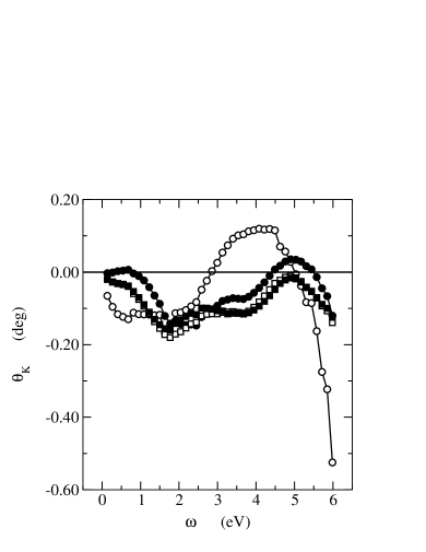
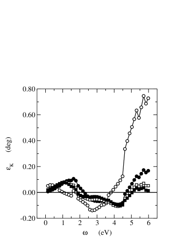
Figure 2: Complex Kerr effect for the $\mathrm{Co}\mid\mathrm{Pt}_{m}$ layered system with $m=0\ (\circ)$, 1 ($\bullet$), 2 ($\scriptstyle\square$), 3 ($\scriptstyle\blacksquare$) Pt–layers below the surface Co–layer (left panel) and separately for $m=3$ (right panel). $\delta=0.048$ Ryd, $T$ = 300 K and $\varepsilon_{z}=\varepsilon_{\vec{k}}=10^{-3}$ a.u., respectively.

The frequency dependence of $\theta_{\mathrm{K}}$ and $\varepsilon_{\mathrm{K}}$ in case of $\mathrm{Co}\mid\mathrm{Pt}_{m}$ surface layered system for different number of Pt buffer layers ($m=0,\ldots,3$) is shown in Fig. 2. As a general trend of these curves, it can be observed, that apart from the $m=0$ situation at low photon energies, our calculations are in agreement with the experimental fact, that the MOKE decreases, if the thickness of the buffer Pt increases Gao et al. (1998).

In fact, $m=0$ means, that one considers only the surface Co–layer in the calculations, i.e., Eqs. (20) and (21) are taken for $n=1$. Although in this case, the layer–resolved optical conductivity equals $\Sigma_{\mu\nu}(\omega)$, the corresponding Kerr spectrum is the most peculiar one in comparison with the results obtained for $m\geq 1$. Once the contribution of different Pt buffer layers below the surface are accounted for ($m\geq 1$), the complex Kerr angle changes dramatically in the whole frequency range and the calculated MOKE for $\mathrm{Co}\mid\mathrm{Pt}_{m=3}$, see right panels in Fig. 2, possesses already the features known from the experiments: $\theta_{\mathrm{K}}$ has two typical, local minima about 2 and 4 eV and $\varepsilon_{\mathrm{K}}$ has a flat region in–between two, local extrema in the middle of the frequency range Uba et al. (1996). The frequency width, however, is smaller than that known from experiments. Below 1 eV and above 5 eV our theoretical spectra are richer in fine details than the experimental data Ebert et al. (1998). Finally, it should be mentioned that, both the Kerr rotation angle and ellipticity are approximatively three times smaller than those measured for thin films of Co–Pt alloy Weller (1996).

To understand this, we introduce layer–resolved complex Kerr angles by using instead of $\Sigma_{\mu\nu}(\omega)$ in Eq. (22), the layer–resolved $\Sigma^{p}_{\mu\nu}(\omega)$, i.e.,

$$\Phi^{p}_{\mathrm{K}}=\theta^{\,p}_{\mathrm{K}}+i\varepsilon^{\,p}_{\mathrm{K}}=\dfrac{\Sigma^{\,p}_{\mathrm{xy}}(\omega)}{\Sigma^{\,p}_{\mathrm{xx}}(\omega)}\left[1+\dfrac{4\pi i}{\omega}\,\Sigma^{\,p}_{\mathrm{xx}}(\omega)\right]^{-\frac{1}{2}}\quad(p=1,\ldots,n)\ .$$ (23)

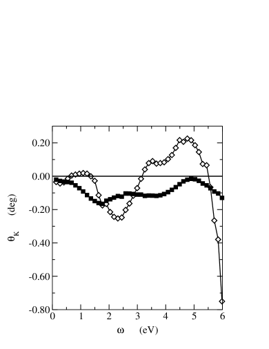
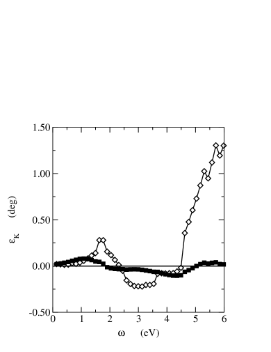
Figure 3: Layer–resolved complex Kerr effect for $\mathrm{Co}\mid\mathrm{Pt}_{m=3}$. In the left panel the Kerr spectra resolved for the surface Co–layer ($\scriptstyle\Diamond$) are compared with that of the layered system ($\scriptstyle\blacksquare$). The right panel show the complex Kerr effect arising from the Pt–layers: $\blacktriangle$ refers to the Kerr spectra resolved for the first Pt–layer below the surface, $\ast$ for the second Pt–layer and $\blacktriangledown$ for the last Pt–layer, respectively.

For $\mathrm{Co}\mid\mathrm{Pt}_{m=3}$, $\Phi^{p}_{\mathrm{K}}$ is plotted in Fig. 3. In contrast to a homogeneous system, like bcc–Fe or fcc–Co Huhne and Ebert (1999), it is found that the surface resolved MOKE cannot predict correctly the complex Kerr effect in our inhomogeneous, surface layered system $\mathrm{Co}\mid\mathrm{Pt}_{m=3}$, see left panels of Fig. 3. Inspecting the layer–resolved complex Kerr angles of the three Pt–layers (right panels in Fig. 3), it can be seen that both $\theta^{\,p}_{\mathrm{K}}$ and $\varepsilon^{\,p}_{\mathrm{K}}$ of the first Pt–layer below the surface Co–layer is in the experimental range Weller (1996). This shows that the first buffer layer is as important as the magnetic surface in an inhomogeneous layered system. Thus in order to exploit the relatively big MOKE in the first buffer layer, one has to bring Pt into the surface Co–layer, e.g. by alloying, and has to prepare thin films. This theoretical finding is completely in–line with the known experimental facts Hatwar et al. (1997).

In addition, we have also studied the variation of MOKE in $\mathrm{Co}\mid\mathrm{Pt}_{m}$ with the thickness of the Pt buffer for $\hbar\omega=0.68$ eV. The change in the layer–resolved MOKE for $m$ up to $15$ is given in Fig. 4. The $\mathrm{Co}\mid\mathrm{Pt}_{m}$ system has only six Pt–layers below the surface included self–consistently and the other Pt–layers are all bulk–like. This construction is based on the fact, that no changes occur neither in MOKE nor in the optical conductivity, if the system has more than six self–consistently included Pt–layers. (Test calculations were carried out for $\mathrm{Co}\mid\mathrm{Pt}_{m=9}$ and $\hbar\omega=0.68$ eV by changing the number of bulk–like Pt-layers in the system.)

As can be seen from Fig. 4, the layer–resolved complex Kerr angles up to nine (ten) Pt mono–layers do not depend linearly on the thickness of the Pt buffer. This is in agreement with other, ab–initio Blaas et al. (2000) and model Bruno et al. (1999) magneto–transport calculations ($\omega=0$) for different multilayer systems, but does not confirm the situation found performing super–cell calculations Perlov and Ebert (2000), where linearity of the surface resolved optical conductivity seems to occur after a few layers.

We have found, that the Kerr angle of the surface Co–layer increases with the thickness of Pt, whereas that of the first Pt–layer below the surface, decreases and the opposite holds for the layer–resolved Kerr ellipticity. Although, these two layers provide the main contributions to the MOKE in $\mathrm{Co}\mid\mathrm{Pt}_{m}$, they alone are not sufficient to describe the complex Kerr angle of the whole system (over nine Pt–layers), because at least twelve Pt–layers are needed to get $\theta_{\mathrm{K}}$ and $\varepsilon_{\mathrm{K}}$ stabilized around -0.005 and 0.009 deg, respectively. The change in the surface resolved MOKE with respect to $m$ is compensated mainly by the change in the layer–resolved MOKE arising from the first non–magnetic layer below the surface, and hence $\theta_{\mathrm{K}}$ and $\varepsilon_{\mathrm{K}}$ finally are converging, for simplicity the layer–resolved MOKE of the Pt–layers below the third one are not shown in Fig. 4. They are situated always in–between the results obtained for the surface Co– and the first Pt–layer below. The deeper the Pt–layer, the smaller its MOKE is, such that the contribution arising from a Pt–layer below the twelve–th layer has a really neglectable influence on the total MOKE.

Finally, in Fig. 5 we show that both, the layer–resolved and the total optical conductivity tensor, respectively, can indeed be computed for $\omega=0$ with a finite life–time broadening by means of the contour integration technique, see also Section 2.3. As can be seen from Fig. 5, the imaginary parts of all $\Sigma^{p}_{\mu\nu}(\omega=0)$ and $\Sigma_{\mu\nu}(\omega=0)$ vanish (with an accuracy of $10^{-3}\,\mathrm{fs}^{-1}$), whereas the real parts of the same quantities remain finite. However, these values cannot be used to calculate the MOKE based on Eqs. (22) and (23), because these expressions are diverging in the static limit.

5 Summary

The contour integration technique applied to Luttinger’s formalism for the optical conductivity tensor has been extended to electric fields with arbitrary polarizations and is shown to straightforwardly account for both the inter– and intra–band contribution. Hence within our technique there is no need to approximate the intra–band contribution by the so–called semi–empirical Drude term. The optical conductivity tensor for finite life–time broadening can be computed also in the zero frequency limit, however, the dc conductivity cannot be obtained integrating in the complex energy plane. The contour integration technique was also completed here in deriving formulae for the current–current correlation function at zero frequency and vanishing life–time broadening ($\zeta=0$).

Introducing the concept of the layer–resolved complex Kerr angles and computing the magneto–optical Kerr effect for the $\mathrm{Co}\mid\mathrm{Pt}_{m}$ surface layered system in polar geometry, we have shown that (1) the layer–resolved complex Kerr angle for the ferromagnetic surface alone cannot predict correctly the magneto–optical Kerr effect in inhomogeneous multilayers. In the case of $\mathrm{Co}\mid\mathrm{Pt}_{m}$ the first Pt–layer below the surface is as important for the polar MOKE as the ferromagnetic surface Co–layer itself. (2) The Kerr spectra of $\mathrm{Co}\mid\mathrm{Pt}_{m=3}$ possess all the known, experimental characteristics, but in order to exploit the relatively big complex Kerr angle arising from the first Pt–layer below the surface, one has to consider a Co–Pt alloy at the surface.

In addition, it was also shown that the layer–resolved MOKE shows a non–linear dependence with respect to the thickness of the buffer Pt up to $m=9$ for $\mathrm{Co}\mid\mathrm{Pt}_{m}$; only for $m\geq 12$ the complex Kerr angle is fully converged.

Finally, we have demonstrated that the contour integration technique developed for the Luttinger formalism can be used straightforwardly with a finite life–time broadening in the zero frequency limit. Calculations performed provide a purely real optical conductivity tensor at zero frequency.

6 Acknowledgements

This work was supported by the Austrian Ministry of Science (Contract No. 45.451/1-III/B/8a/99) and by the Research and Technological Cooperation Project between Austria and Hungary (Contract No. A-35/98). One of the authors (L.S.) is also indebted to partial support by the Hungarian National Science Foundation (Contract No. OTKA T030240).

Figure 1: Selection of contour $\Gamma_{1}$ and $\Gamma_{2}$. $\varepsilon_{m}$ and $\varepsilon_{n}$ are eigenvalues of the Hamiltonian, $\zeta=\hbar\omega+i\delta$, with $\omega$ being the frequency and $\delta$ the life–time broadening. $\varepsilon_{\mathrm{F}}$ is the Fermi level, $\varepsilon_{\mathrm{b}}$ the bottom valence band energy and $\varepsilon_{\mathrm{u}}=\varepsilon_{\mathrm{F}}+\xi k_{\mathrm{B}}T$ ($\xi\in\mathbb{N}$). $z_{k}=\varepsilon_{\mathrm{F}}+i\left(2k-1\right)\delta_{T}$ are Matsubara poles with $k=0,\pm 1,\pm 2,\ldots$ and $\delta_{T}=\pi k_{\mathrm{B}}T$. $\delta_{1,2}$ were selected to fulfill the condition given by Eq. (10).

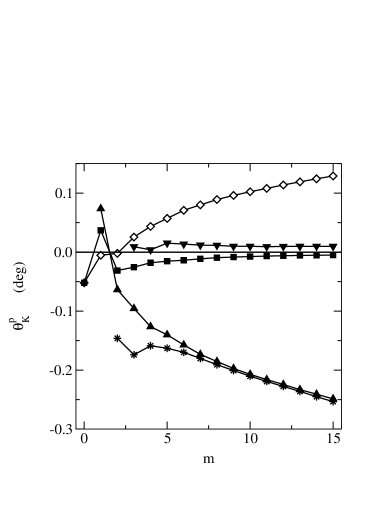
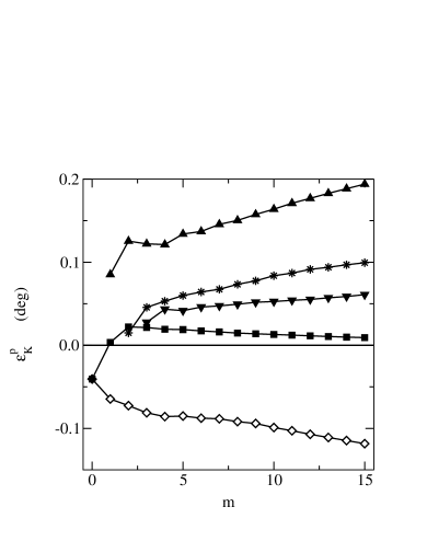
Figure 4: Total and layer–resolved complex Kerr angle for $\hbar\omega=0.68$ eV and the $\mathrm{Co}\mid\mathrm{Pt}_{m}$ multilayer ($m=0,\ldots,15$), containing below the surface Co–layer six self–consistently included Pt–layers followed by bulk–like layers. (The used symbols represent the same type of data as in Fig. 3.)

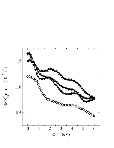
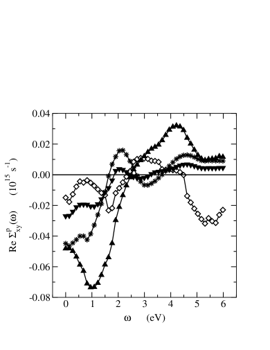
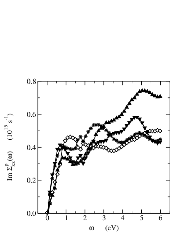
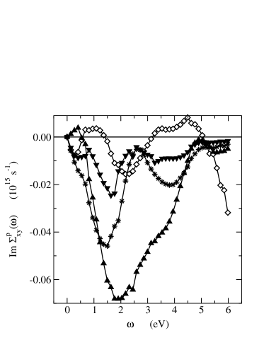
Figure 5: Real and imaginary part of the total and layer–resolved optical conductivity for $\mathrm{Co}\mid\mathrm{Pt}_{m=3}$. The optical conductivity resolved for the surface Co–layer is given by $\scriptstyle\Diamond$ and that resolved for the Pt–layers by $\blacktriangle$, $\ast$ and $\blacktriangledown$, respectively. The optical conductivity of the multilayer is represented by $\ast$.

References

- (1)
- Abramowitz and Stegun (1972) Abramowitz, M. and I.A. Stegun (1972). Handbook of Mathematical Functions with Formulas, Graphs and Mathematical Tables. Dover, New York.
- Bruno et al. (1999) Bruno, P., H. Itoh, J. Inoue and S. Nonoya (1999). Influence of disorder on the perpendicular magnetoresistance of magnetic multilayers. J. Magn. Magn. Materials, 198–199, 46.
- Bertero and Sinclair (1994) Bertero, G.A. and R. Sinclair (1994). Structure–property correlations in Pt/Co multilayers for magneto–optic recording. J. Magn. Magn. Materials, 134, 173.
- Blaas et al. (2000) Blaas, C., L. Szunyogh, P. Weinberger, C. Sommers and P.M. Levy (2000). Electrical transport properties of bulk NicFe1-c alloys and related spin–valve systems. Phys. Rev. B, manuscript no. BU7531.
- Butler (1985) Butler, W.H. (1985). Theory of electronic transport in random alloys: Korringa–Kohn–Rostoker coherent–potential approximation. Phys. Rev. B, 31, 3260.
- Blaas et al. (1999) Blaas, C., P. Weinberger, L. Szunyogh, P.M. Levy and C.B. Sommers (1999). Ab initio calculations of magnetotransport for magnetic multilayers. Phys. Rev. B, 60, 492.
- Butler et al. (1994) Butler, W.H., X.G. Zhang, D.M.C. Nicholson and J.M. MacLaren (1994). Theory of transport in inhomogeneous systems and application to magnetic multilayer systems. J. Appl. Physics, 76, 6808.
- Callaway (1974) Callaway, J. (1974). Quantum Theory of the Solid State part B. Academic Press, New York.
- Calvetti et al. (2000) Calvetti, D., G.H. Golub, W.B. Gragg and L. Reichel (2000). Computation of Gauss–Konrod quadrature rules. Math. Comput., 69, 1035.
- Daalderop et al. (1988) Daalderop, G.H.O., F.M. Mueller, R.C. Albers and A.M. Boring (1988). Prediction of a large polar Kerr angle in NiUSn. Appl. Physics Lett., 52, 1636.
- Ebert et al. (1998) Ebert, H., A. Perlov, A.N. Yaresko, V.N. Antonov and S. Uba (1998). Theoretical investigations on the magneto-optical properties of transition metal multilayer and surface systems. Mat. Res. Soc. Symp. Proc., 475, 407.
- Eykholt (1986) Eykholt, R. (1986). Extension of the Kubo formula for the electrical conductivity tensor to arbitrary polarizations of the electric field. Phys. Rev. B, 34, 6669.
- Gao et al. (1998) Gao, X., M.J. DeVries, D.W. Thompson and J.A. Woollam (1998). Thickness dependence of interfacial magneto–optic effects in PtCo multilayers. J. Appl. Physics, 83, 6747.
- Guo and Ebert (1995) Guo, G.Y. and H. Ebert (1995). Band theoretical investigation of the magneto-optical Kerr effect in Fe and Co multilayers. Phys. Rev. B, 51, 12633.
- Greenwood (1958) Greenwood, D.A. (1958). The Boltzmann equation in the theory of electrical conduction in metals. Proc. Phys. Soc., 71, 585.
- Huhne and Ebert (1999) Huhne, T. and H. Ebert (1999). Fully relativistic description of the magneto–optical properties of arbitrary layered systems. Phys. Rev. B, 60, 12982.
- Hatwar et al. (1997) Hatwar, T.K., Y.S. Tyan and C.F. Brucker (1997). High–performance Co/Pt multilayer magneto–optical disk using ultrathin seed layers. J. Appl. Physics, 81, 3839.
- Yu-Kuang Hu (1993) Yu-Kuang Hu, B. (1993). Simple derivation of a general relationship between imaginary- and real-time Green’s correlation functions. Am. J. Phys., 61, 457.
- Hama and Watanabe (1992) Hama, J. and M. Watanabe (1992). General formulae for the special points and their weighting in k-space integration. J. Phys.: Condensed Matter, 4, 4583.
- Kubo (1957) Kubo, R. (1957). Statistical–mechanical theory of irreversible processes I. J. Phys. Soc. Japan, 12, 570.
- Kubo (1966) Kubo, R. (1966). The fluctuation–dissipation theorem. Rep. Prog. Phys., 29, 255.
- Laurie (1997) Laurie, D.P. (1997). Calculation of Gauss–Konrod quadrature rules. Math. Comput., 66, 1133.
- Lax (1958) Lax, M. (1958). Generalized mobility theory. Phys. Rev., 109, 1921.
- Luttinger (1964) Luttinger, J.M. (1964). Theory of thermal transport coefficients. Phys. Rev., 135A, 1505.
- Luttinger (1967) Luttinger, J.M. (1967). Transport theory. In Mathematical Methods in Solid State and Superfluid Theory, Oliver and Boyd, Edingburgh, Chap. 4, pp. 157.
- Mahan (1990) Mahan, G.D. (1990). Many–Particle Physics. Plenum Press, New York.
- Mansuripur (1995) Mansuripur, M. (1995). The Principles of Magneto-Optical Recording. Cambridge University Press, Cambridge.
- Nicholson et al. (1994) Nicholson, D.M.C., G.M. Stocks, Y. Wang, W.A. Shelton, Z. Szotek and W.M. Temmerman (1994). Stationary nature of the density–functional free energy: Application to accelerated multiple–scattering calculations. Phys. Rev. B, 50, 14686.
- Oppeneer et al. (1992) Oppeneer, P.M., T. Maurer, J. Sticht and J. Kübler (1992). Ab initio calculated magneto–optical Kerr effect of ferromagnetic metals: Fe and Ni. Phys. Rev. B, 45, 10924.
- Oppeneer (1999) Oppeneer, P.M. (1999). Theory of the magneto–optical Kerr effect in ferromagnetic compounds. Habilitationsschrift, Technische Universität Dresden.
- Perlov and Ebert (2000) Perlov, A.Ya. and H. Ebert (2000). Layer–resolved optical conductivity of magnetic multilayers. Europhys. Lett., 52, 108.
- Press et al. (1992) Press, W.H., B.P. Flannery, S.A. Teukolsky and W.T. Vetterling (1992). Numerical Recipes in Fortran: The Art of Scientific Computing. Cambridge University Press, Cambridge.
- Pustogowa et al. (1999) Pustogowa, U., J. Zabloudil, C. Uiberacker, C. Blaas, P. Weinberger, L. Szunyogh and C. Sommers (1999). Magnetic properties of thin films of Co and of (CoPt) superstructures on Pt(100) and Pt(111). Phys. Rev. B, 60, 414.
- Reim and Schoenes (1990) Reim, W. and J. Schoenes (1990). Magneto–optical spectroscopy of –electron systems. In K.H.J. Buschow and E.P. Wohlfarth (Eds.), Ferromagnetic Materials, Vol. 5, North-Holland, Amsterdam, Chap. 2, pp. 133.
- Szunyogh et al. (1995) Szunyogh, L., B. Újfalussy and P. Weinberger (1995). Magnetic anisotropy of iron multilayers on Au(001). Phys. Rev. B, 51, 9552.
- Szunyogh et al. (1994) Szunyogh, L., B. Újfalussy, P. Weinberger and J. Kollár (1994). Self–consistent localized KKR scheme for surfaces and interfaces. Phys. Rev. B, 49, 2721.
- Szunyogh and Weinberger (1999) Szunyogh, L. and P. Weinberger (1999). Evaluation of the optical conductivity tensor in terms of contour integrations. J. Phys.: Condensed Matter, 11, 10451.
- Újfalussy et al. (1995) Újfalussy, B., L. Szunyogh and P. Weinberger (1995). Magnetism of 4d and 5d adlayers on Ag(001) and Au(001): comparison between a non–relativistic and a fully relativistic approach. Phys. Rev. B, 51, 12836.
- Uba et al. (1996) Uba, S., L. Uba, A.N. Yaresko, A.Ya. Perlov, V.N. Antonov and R. Gontarz (1996). Optical and magneto–optical properties of Co/Pt multilayers. Phys. Rev. B, 53, 6526.
- Vernes et al. (2000) Vernes, A., L. Szunyogh and P. Weinberger (2000). Numerically improved computational scheme for the optical conductivity tensor in layered systems. submitted to J. Phys.: Condensed Matter.
- Wang and Callaway (1974) Wang, C.S. and J. Callaway (1974). Band structure of nickel: spin-orbit coupling, the Fermi surface, and the optical conductivity. Phys. Rev. B, 9, 4897.
- Weinberger (1990) Weinberger, P. (1990). Electron Scattering Theory for Ordered and Disordered Matter. Oxford University Press, Oxford.
- Weller (1996) Weller, D. (1996). Magneto–optical Kerr spectroscopy of transition metal alloy and compound films. In H. Ebert and G. Schütz (Eds.) Spin-orbit Influenced Spectroscopies of Magnetic Solids, Vol. 466 of Lecture Notes in Physics, Springer, Berlin, pp. 1.
- Weinberger et al. (1996) Weinberger, P., P.M. Levy, J. Banhart, L. Szunyogh and B. Újfalussy (1996). Band structure and electrical conductivity of disordered layered systems. J. Phys.: Condensed Matter, 8, 7677.
- Wildberger et al. (1995) Wildberger, K., P. Lang, R. Zeller and P.H. Dederichs (1995). Fermi–Dirac distribution in ab initio Green’s–function calculations. Phys. Rev. B, 52, 11502.