Redundancy and synergy arising from correlations in large ensembles

Abstract

Multielectrode arrays allow recording of the activity of many single neurons, from which correlations can be calculated. The functional roles of correlations can be revealed by the measures of the information conveyed by neuronal activity; a simple formula has been shown to discriminate the information transmitted by individual spikes from the positive or negative contributions due to correlations (Panzeri et al, Proc. Roy. Soc. B., 266: 1001–1012 (1999)). The formula quantifies the corrections to the single-unit instantaneous information rate which result from correlations in spike emission between pairs of neurons. Positive corrections imply synergy, while negative corrections indicate redundancy. Here, this analysis, previously applied to recordings from small ensembles, is developed further by considering a model of a large ensemble, in which correlations among the signal and noise components of neuronal firing are small in absolute value and entirely random in origin. Even such small random correlations are shown to lead to large possible synergy or redundancy, whenever the time window for extracting information from neuronal firing extends to the order of the mean interspike interval. In addition, a sample of recordings from rat barrel cortex illustrates the mean time window at which such ‘corrections’ dominate when correlations are, as often in the real brain, neither random nor small. The presence of this kind of correlations for a large ensemble of cells restricts further the time of validity of the expansion, unless what is decodable by the receiver is also taken into account.

1 Do correlations convey more information than do rates alone?

Our intuition often brings us to regard neurons as independent actors in the business of information processing. We are then reminded of the potential for intricate mutual dependence in their activity, stemming from common inputs and from interconnections, and are finally brought to consider correlations as sources of much richer, although somewhat hidden, information about what a neural ensemble is really doing. Now that the recording of multiple single units is common practice in many laboratories, correlations in their activity can be measured and their role in information processing can be elucidated case by case. Is the information conveyed by the activity of an ensemble of neurons determined solely by the number of spikes fired by each cell as could be quantified also with non-simultaneous recordings [1]; or do correlations in the emission of action potentials also play a significant role?

Experimental evidence on the role of correlations in neural coding of sensory events, or of internal states, has been largely confined to ensembles of very few cells. Their contribution has been said to be positive, i.e. the information contained in the ensemble response is greater than the sum of contributions of single cells (synergy)  [2, 3, 4, 5, 6], or negative (redundancy) [7, 8, 9]. Thus, specific examples can be found of correlations that limit the fidelity of signal transmission, and others that carry additional information. Another view is that usually correlations do not make much of a difference in either direction [10, 11, 12] and that their presence can be regarded as a kind of random noise. In this paper, we show that even when correlations are of a completely random nature they may contribute very substantially, and to some extent predictably, to information transmission.

To discuss this point we must first quantify the amount of information contained in the neural response. Information theory [13] provides one framework for describing mathematically the process of information transmission, and it has been applied successfully to the analysis of neuronal recordings [12, 14, 15, 16]. Consider a stimulus taken from a finite discrete set $\cal{S}$ with $S$ elements, each stimulus $s$ occurring with probability $P(s)$. The probability of response ${\bf r}$ (the ensemble activity, imagined as the firing rate vector) is $P({\bf r})$, and the joint probability distribution is $P(s,{\bf r})$. The mutual information between the set of stimuli $\cal{S}$ and the response is

$$I(t)=\sum_{s\in\cal{S}}\sum_{{\bf r}}P(s,{\bf r})\log_{2}\frac{P(s,{\bf r})}{P(s)P({\bf r})}$$ (1)

where $t$ is the length of the time window for recording the response ${\bf r}$.

We study here the contribution of correlations to such mutual information. In the $t\to 0$ limit, the mutual information can be broken down into a firing rates and correlations components, as shown by Panzeri et al. [17] and summarized in the next section. The correlation-dependent part can be further expanded by considering “small” correlation coefficients (see Section 3). In this (additional) limit approximation the effects of correlations can be analyzed and it will be seen that even if they are random they give large contributions to the total information. The number of second-order (pairwise) correlation terms in the information expansion in fact grows as $C^{2}$, where $C$ is the number of cells, while contributions that depend only on individual cell firing rates of course grow linearly with $C$. As a result, as shown by Panzeri et al. [24], the time window to which the expansion is applicable shrinks as the number of cells increases, and conversely the overall effect of correlation grows. We complement this derivation by analysing (see Section 4) the response of cells in the rat somatosensory barrel cortex during the response to deflections of the vibrassae. Conclusions about the general applicability of correlation measures to information transmission are drawn in the last section.

2 The short time expansion

In the limit $t\to 0$, following Ref. [17], the information carried by the population response can be expanded in a Taylor series

$$I(t)=t\;I_{t}+{t^{2}\over 2}\;I_{tt}+\dots$$ (2)

There is no zero order term, as no information can be transmitted in a null time-window. Higher order terms (see Ref. [18]) are not considered here, but they could be included in a straightforward extension of this approach.

Assuming that the conditional probability of a spike being emitted by cell $i$, $n_{i}=1$, given that cell $j$ has fired scales proportionally to $t$, i.e.:

$$P(n_{i}(s)=1|n_{j}=1;s)\equiv\overline{r}_{i}(s)t(1+\gamma_{ij}(s))$$ (3)

(where the $\gamma_{ij}(s)$ coefficient quantifies correlations) the expansion (2) becomes an expansion in the total number of spikes emitted by an assembly of neurons (see Ref. [17] for details). Briefly, the procedure is the following: the expression for $P(n)$ (3) is inserted in the Shannon formula for information, Eq.(1), whose logarithm is then expanded in a power series. All terms, with the same power of $t$, are grouped and compared to Eq.(2), to extract first and second order derivatives.

The first time derivative (i.e. the information rate) depends only on the firing rates averaged over trials with the same stimulus, denoted as $\overline{r}_{i}(s)$

$$I_{t} = \sum_{i=1}^{C}\left<\overline{r}_{i}(s)\log_{2}{\overline{r}_{i}(s)\over\left<\overline{r}_{i}(s^{\prime})\right>_{s^{\prime}}}~{}\right>_{s}$$

i.e. the sum of the information rate of each single cell [19, 20].

The second derivative breaks into three components

$$I_{tt}=I_{tt}^{(1)}+I_{tt}^{(2)}+I_{tt}^{(3)}$$

These terms depend on two different kinds of correlations, usually termed ‘signal’ and ‘noise’ correlations [7]. ‘Noise’ correlations are pairwise correlations in the response variability, i.e. a measure of the tendency of both of the cells to fire more (or less) during the same trial, compared to their average response over many trials with the same stimulus. For short time windows this is a measure of the synchronization of the cells. We introduce the ‘scaled cross-correlation density’ [21], i.e. the amount of trial by trial concurrent firing between different cells, compared to that expected in the uncorrelated case

$$\gamma_{ij}(s)={\overline{{r}_{i}(s){r}_{j}(s)}\over\overline{r}_{i}(s)\overline{r}_{j}(s)}-1.$$

This coefficient can vary from $-1$ to $+\infty$; negative values indicate anticorrelation, whereas positive $\gamma_{ij}$ values indicate correlation. For $i=j$, the ‘scaled autocorrelation coefficient’ $\gamma_{ii}$ gives the probability of observing a spike emission, given that the same cell has already fired in the same time window; i.e.

$$\gamma_{ii}(s)={\overline{{r}^{2}}_{i}(s)-\overline{r}_{i}(s)\over\overline{r}_{i}^{2}(s)}-1$$

The relationship with alternative cross-correlation coefficients, like the Pearson correlation, is discussed in Ref. [17].

‘Signal’ correlations measure the tendency of pairs of cells to respond more (or less) to the same stimuli in the stimulus set. As in the previous case we introduce the signal cross-correlation coefficient $\nu_{ij}$,

$$\nu_{ij}={<\overline{r}_{i}(s)\overline{r}_{j}(s)>_{s}\over<\overline{r}_{i}(s)>_{s}<\overline{r}_{j}(s)>_{s}}-1$$ (4)

and, similarly, we define the autocorrelation coefficient $\nu_{ii}$.

The first term of $I_{tt}$ again depends only on the mean rates:

$$I_{tt}^{(1)}={1\over\ln 2}\sum_{i=1}^{C}\sum_{j=i}^{C}\left<\overline{r}_{i}(s)\right>_{s}\left<\overline{r}_{j}(s)\right>_{s}\biggl{[}\nu_{ij}+(1+\nu_{ij})\ln({1\over 1+\nu_{ij}})\biggr{]}$$

The second term is non-zero only when correlations are present both in the noise (even if they are stimulus-independent) and in the signal

$$I_{tt}^{(2)}={1\over\ln 2}\sum_{i=1}^{C}\sum_{j=i}^{C}\biggl{[}\left<\overline{r}_{i}(s)\overline{r}_{j}(s)\gamma_{ij}(s)\right>_{s}\biggr{]}\ln({1\over 1+\nu_{ij}}).$$

The third term contributes only if correlations are stimulus-dependent

$$I_{tt}^{(3)} = {1\over\ln 2}\sum_{i=1}^{C}\sum_{j=i}^{C}\left<\overline{r}_{i}(s)\overline{r}_{j}(s)(1+\gamma_{ij}(s))\ln\left[{\left<\overline{r}_{i}(s^{\prime})\overline{r}_{j}(s^{\prime})\right>_{s^{\prime}}(1+\gamma_{ij}(s))\over\left<\overline{r}_{i}(s^{\prime})\overline{r}_{j}(s^{\prime})(1+\gamma_{ij}(s^{\prime}))\right>_{s^{\prime}}}\right]\right>_{s}.$$

The sum $I_{t}t+\frac{1}{2}I_{tt}^{(1)}t^{2}$ depends only on average firing rates, $\overline{r}_{i}(s)$, (rate only contribution) and its first term is always greater than or equal to zero, while $I_{tt}^{(1)}$ is always less than or equal to zero.

In the presence of correlations, i.e. non zero $\gamma_{ij}$ and $\nu_{ij}$, more information may be available when observing simultaneously the responses of many cells, than when observing them separately: synergy. For two cells, it can happen due to positive correlations in the variability, if the mean rates to different stimuli are anticorrelated, or vice-versa. If the signs of signal and noise correlations are the same, the result is always redundancy. Quantitatively, the impact of correlations is minimal when the mean responses are only weakly correlated across the stimulus set.

The time range of validity of the expansion (2) is limited by the requirement that second order terms be small with respect to first order ones, and successive orders be negligible. Since at order $n$ there are $C^{n}$ terms with $C$ cells, the applicability of the short time limit contracts for larger populations.

3 Large number of cells

Let us investigate the role of correlations in the transmission of information by large populations of cells. For a few cells, all cases of synergy or redundancy are possible if the correlations are properly engineered, in simulations, or if, in experiments, the appropriate special case is recorded. The outcome of the information analysis simply reflects the peculiarity of each case. With large populations, one may hope to have a better grasp of generic, or typical, cases, more indicative of conditions prevailing at the level of, say, a given cortical module, such as a column.

Consider a ‘null’ hypothesis model of a large population: purely random correlations; i.e. correlations that were not designed to play any special role in the system being analyzed.

In this null hypothesis, signal correlations $\nu_{ij}$ can be thought of as arising from a random walk with $S$ steps (the number of stimuli). Such a random walk of positive and negative steps typically spans a range of size $\sqrt{S}$. The $\nu_{ij}$ have zero average, while the squares $\nu_{ij}^{2}$ still differ from zero on average, since they are positive. Noise correlations may be thought to arise from stimulus-independent terms, $\gamma_{ij}$ (which may well be large), and from stimulus-dependent contributions, which we denote $\delta\gamma_{ij}(s)$ and which might be expected to get smaller when more trials per stimulus are available, and whose squares again would be expected to span the range of a random walk (whose steps are now the different trials). The effect of such null hypothesis correlations on information transmission can be gauged by further expanding $I_{tt}$ in the small parameters $\nu_{ij}$ and $\delta\gamma_{ij}(s)$, i.e. assuming $|\nu_{ij}|<<1$ and $|\delta\gamma_{ij}(s)|<<1$.

Consider, first, the expansion of $I_{tt}^{(1)}$, that does not depend on $\gamma_{ij}(s)$. Expanding in powers of $\nu_{ij}$ and neglecting terms of order $3$ or higher, we easily get:

$$I_{tt}^{(1)} = -{1\over\ln 2}\sum_{i=1}^{C}\sum_{j=i}^{C}\left<\overline{r}_{i}(s)\right>_{s}\left<\overline{r}_{j}(s)\right>_{s}\nu_{ij}^{2}$$ (5)

The second contribution of $I_{tt}$, up to the second order in $\nu_{ij}$, is

$$I_{tt}^{(2)} = -{1\over\ln 2}\sum_{i=1}^{C}\sum_{j=i}^{C}\biggl{[}(1+\gamma_{ij})\left<\overline{r}_{i}(s)\right>_{s}\left<\overline{r}_{j}(s)\right>_{s}\nu_{ij}^{2}+$$ (6)

$$+ (1+\gamma_{ij})\left<\overline{r}_{i}(s)\right>_{s}\left<\overline{r}_{j}(s)\right>_{s}\nu_{ij}+\left<\overline{r}_{i}(s)\overline{r}_{j}(s)\delta\gamma_{ij}(s)\right>_{s}\nu_{ij}\biggr{]}$$ (7)

The third contribution, $I_{tt}^{(3)}$ is more complicated, as an expansion in $\delta\gamma_{ij}(s)$ is required as well. Expanding the logarithm in these small parameters up to second order we get:

$$I_{tt}^{(3)} = {1\over{\ln 2}}\sum_{i=1}^{C}\sum_{j=i}^{C}{1\over{1+\gamma_{ij}}}\biggl{[}\left<\overline{r}_{i}(s)\overline{r}_{j}(s)\delta\gamma_{ij}(s)^{2}\right>_{s}-\frac{\left<\overline{r}_{i}(s)\overline{r}_{j}(s)\delta\gamma_{ij}(s)\right>^{2}_{s}}{\left<\overline{r}_{i}(s)\overline{r}_{j}(s)\right>_{s}}\biggr{]}$$ (8)

Introducing the average on stimuli weighted on the product of the normalized firing rates, $\overline{r}_{i}(s)\overline{r}_{j}(s)/\left<\overline{r}_{i}(s)\overline{r}_{j}(s)\right>_{s}$, that is

$$\left<\delta\gamma_{ij}(s)\right>_{\{i,j\},s}=\frac{1}{S}\sum_{i=1}^{S}\frac{\overline{r}_{i}(s)\overline{r}_{j}(s)}{\left<\overline{r}_{i}(s)\overline{r}_{j}(s)\right>_{s}}\delta\gamma_{ij}(s)$$

we obtain, from Eq. (8),

$$I_{tt}^{(3)}={1\over{\ln 2}}\sum_{i=1}^{C}\sum_{j=i}^{C}\frac{(\nu_{ij}+1)\left<\overline{r}_{i}(s)\right>_{s}\left<\overline{r}_{j}(s)\right>_{s}}{1+\gamma_{ij}}\biggl{[}\left<\delta\gamma_{ij}(s)^{2}\right>_{\{i,j\},s}-\left<\delta\gamma_{ij}(s)\right>_{\{i,j\},s}^{2}\biggr{]}$$

that is a non-negative quantity, i.e. a synergetic contribution to information. In case of random “noise” correlations, with zero weighted average over the set of stimuli, i.e. $\left<\delta\gamma_{ij}(s)\right>_{\{i,j\},s}=0$, this equation can be re-written,

$$I_{tt}^{(3)}={1\over{\ln 2}}\sum_{i=1}^{C}\sum_{j=i}^{C}\frac{\nu_{ij}+1}{1+\gamma_{ij}}\left<\overline{r}_{i}(s)\right>_{s}\left<\overline{r}_{j}(s)\right>_{s}\left<\delta\gamma_{ij}(s)^{2}\right>_{\{i,j\},s}\equiv\frac{C(C+1)}{2\ln 2}\left<\delta\gamma^{2}\right>_{C}$$ (9)

where we have introduced, to simplify the notation,

$$\left<\delta\gamma^{2}\right>_{C}\equiv\frac{1}{C(C+1)/2}\sum_{i=1}^{C}\sum_{j=i}^{C}\frac{\nu_{ij}+1}{1+\gamma_{ij}}\left<\overline{r}_{i}(s)\right>_{s}\left<\overline{r}_{j}(s)\right>_{s}\left<\delta\gamma_{ij}(s)^{2}\right>_{\{i,j\},s}$$

Assuming purely random signal correlations $\nu_{ij}$ with zero average, we get, summing eqs. (5) and (7),

$$I_{tt}^{(1)}+I_{tt}^{(2)}=-{2\over\ln 2}\sum_{i=1}^{C}\sum_{j=i}^{C}(1+\frac{\gamma_{ij}}{2})\left<\overline{r}_{i}(s)\right>_{s}\left<\overline{r}_{j}(s)\right>_{s}\nu_{ij}^{2}\equiv-\frac{C(C+1)}{\ln 2}\left<\nu^{2}\right>_{C}$$ (10)

where we have introduced (in a similar way as for $\delta\gamma$; these two definitions coincide for $\nu_{ij}$ and $\gamma_{ij}\rightarrow 0$):

$$\left<\nu^{2}\right>_{C}=\frac{1}{C(C+1)/2}\sum_{i=1}^{C}\sum_{j=i}^{C}(1+\frac{\gamma_{ij}}{2})\left<\overline{r}_{i}(s)\right>_{s}\left<\overline{r}_{j}(s)\right>_{s}\nu_{ij}^{2}$$

This contribution (Eq. 10) to information is always negative (redundancy).

Thus the leading contributions of the new Taylor expansion are of two types, both coming as $C(C+1)/2$ terms proportional to $\left<\overline{r}_{i}(s)\right>_{s}\left<\overline{r}_{j}(s)\right>_{s}$. The first one, Eq. (10), is a redundancy term proportional to $\left<\nu^{2}\right>$; the second one, Eq. (9), is a synergy term roughly proportional to $\left<\delta\gamma^{2}\right>$.

These leading contributions to $I_{tt}$ can be compared to first order contributions to the original Taylor expansion in $t$ (i.e., to the $C$ terms in $I_{t}$) in different time ranges. For times $t\approx{\rm ISI}/C$, that is $t\left<\overline{r}\right>\approx 1/C$, first order terms sum up to be of order one bit, while second order terms are smaller (to the extent that $\left<\nu^{2}\right>_{C}$ and $\left<\delta\gamma^{2}\right>_{C}$ are taken to be small). This occurs however over a time range that becomes shorter as more cells are considered, and the total information conveyed by the population remains of order 1 bit.

For times $t\simeq{\rm ISI}$, i.e. $t\left<\overline{r}\right>\approx 1$, first order terms are of order $C$, while second order ones are of order $C^{2}\left<\nu^{2}\right>_{C}$ (with a minus sign, signifying redundancy) and $C^{2}\left<\delta\gamma^{2}\right>_{C}$ (with a plus sign, signifying synergy) respectively. If $\left<\nu^{2}\right>_{C}$ and $\left<\delta\gamma^{2}\right>_{C}$ are not sufficiently small to counteract the additional $C$ factor, these “random” redundancy and synergy contributions will be substantial. Moreover, over the same time ranges leading contributions to $I_{ttt}$ and to the next terms in the Taylor expansion in time may be expected to be substantial. The expansion already will be of limited use by the time most cells have fired just a single spike.

If this bleak conclusion comes from a model with small and random correlations, what is the time range of applicability of the expansion when several real cells are recorded simultaneously?

4 Measuring correlations in rat barrel cortex

We have analyzed many sets of data recorded from rat cortex. Part of the primary somatosensory cortex of the rat (the barrel cortex) is organized in a grid of columns, with each column anatomically and functionally associated with one homologous whisker (vibrissa) on the controlateral side: the column’s neurons respond maximally, on average, to the deflection of this “principal” whisker. In our experiments, in a urethane-anesthetized rat, one whisker was stimulated at 1 Hz, and each deflection lasted for 100 $ms$. The latency (time delay between stimulus onset and the evoked response) in this fast sensory system is usually around $5-10ms$. We present here the complete analysis of a single typical dataset. The physiological methods are described in Ref. [23].

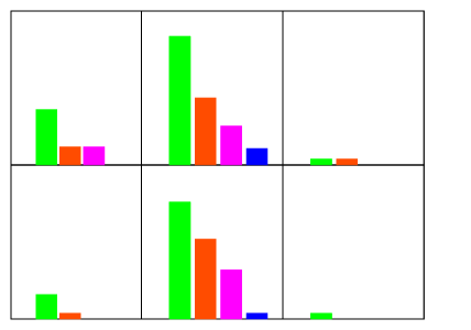
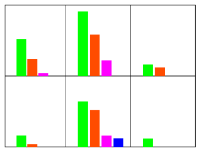
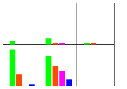
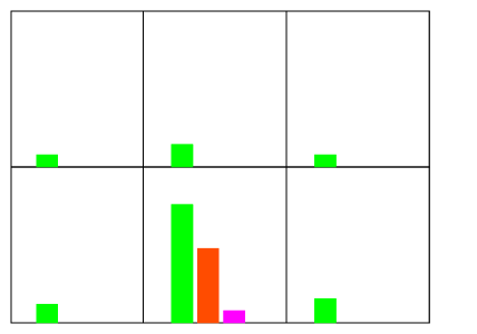
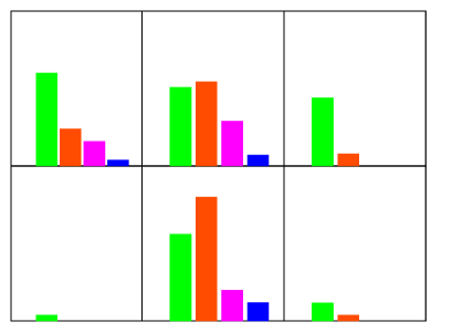
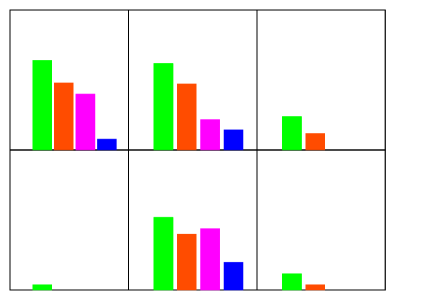
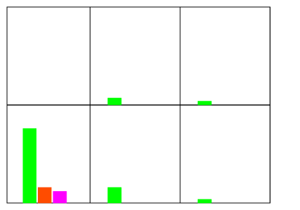
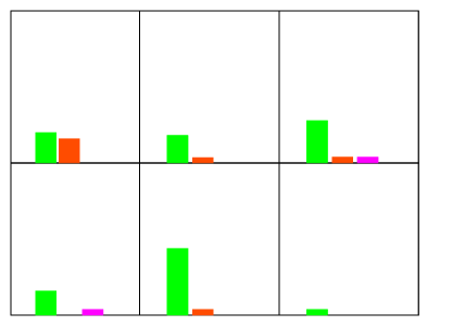
Figure 1: Firing rate distributions (probability of observing a given number of spikes emitted in the time window of $40ms$), for 9 cells and 6 different stimuli (that is, $6$ whisker sites). The bars, from left to right, represent the probability to have ($0$ not shown) $1$, $2$, $3$, or more than $3$ (black bar) spikes during a single stimulus presentation. Maximum $y$-axis set to $0.5$.

For each stimulus site there were $50$ trials and in our analysis we have considered up to $6$ stimulus sites, (i.e. different whiskers) with 12 cells recorded simultaneously. In Fig. 1 we report the firing distributions of 9 of the 12 cells for each of the 6 stimuli. One can immediately note that several cells are most strongly activated by a single whisker, while responding more weakly or not at all to the others. Other cells have less sharply tuned receptive fields. A mixture of sharply tuned and more broadly tuned receptive fields is characteristic of a given population of barrel cortex neurons. We have computed the distribution of $\nu_{ij}$ and $\delta\gamma_{ij}(s)$ for different time windows.

Figure 2: The distribution $P(\nu)$, considering the $\nu_{ij}$ for each cell pair $i$ and $j$. Computed after $30ms$ with 2 stimuli, $50$ trials per stimulus (averaged over all possible pairs from among $6$ stimuli, top left), with all the $6$ stimuli (top right), with $6$ stimuli and after $40ms$ (bottom left) and with $6$ stimuli and after $40ms$ but with only $20$ trials per stimulus (bottom right).

In Fig. 2 we have plotted the distribution of all $\nu_{ij}$. In the first figure (Fig. 2, top, left) we have considered 2 stimuli, taken from the set of $6$ stimuli, and averaged over all the possible pairs. In the following figure (Fig. 2, top, right), where we take all the $6$ stimuli, the distribution is broader ($\sigma=1.2$ vs. $\sigma=0.5$ in the previous case), and the maximum value of $\nu$ is $2.8$ (vs. $1.0$). This larger spread of $\nu$ values can be explained by the fact that most cells have a greater response for one stimulus, and weaker for the other. This can be seen by considering a limit case: two cells $i$ and $j$ fire just to a single stimulus $s^{\prime}$, i.e. $\overline{r}_{i}(s^{\prime})\neq 0$ $\overline{r}_{j}(s^{\prime})\neq 0$ and $\overline{r}_{j}(s)=\overline{r}_{i}(s)=0$ for $s\neq s^{\prime}$. From Eq. (4), we have

$$\nu_{ij}={\frac{1}{S}\sum_{s}\overline{r}_{i}(s)\overline{r}_{j}(s)\over\frac{1}{S}\sum_{s}\overline{r}_{i}(s)\frac{1}{S}\sum_{s}\overline{r}_{j}(s)}-1={\frac{1}{S}\overline{r}_{i}(s^{\prime})\overline{r}_{j}(s^{\prime})\over\frac{1}{S}\overline{r}_{i}(s^{\prime})\frac{1}{S}\overline{r}_{j}(s^{\prime})}-1=S-1$$

As the total number of stimuli $S$ increases, $\nu$ values of the order of $S$ appear, and broaden the distribution. The distribution does not change qualitatively when the time window lengthens, (Fig. 2, bottom, left) at least from $30ms$ to $40ms$, except for a somewhat narrower width with the longer time-window. For very short time windows ($\leq 20ms$) we observe instead a peak at $\nu=0$ and $\nu=-1$ due to the prevalence of cases of zero spikes: when the mean rates of at least one of the two cells are zero to all stimuli $\nu=0$, and when the stimuli, to which each gives a non-zero response, are mismatched, then $\nu=-1$. In the last panel (Fig. 2, bottom, right) we have taken a more limited sample ($20$ trials), which in this case does not significantly change the moments of the distribution.

Figure 3: The distribution $P(\delta\gamma)$, considering all $\delta\gamma_{ij}$ for each cell pair $i$ and $j$ and for each stimulus $s$. Computed after $30ms$ with 2 stimuli, $50$ trials per stimulus (averaged over all possible pairs of $6$ stimuli, top left), with all the $6$ stimuli (top right), with $6$ stimuli and after $40ms$ (bottom left) and with with $6$ stimuli and after $40ms$ but with only $20$ trials per stimulus (bottom right).

The distribution of $\delta\gamma$ is illustrated in Fig. 3. This distribution has $0$ average by definition; we can observe that the spread becomes larger when increasing the number of stimuli from $2$ (Fig. 3, top left) to $6$ (Fig. 3, top right). This derives from having rates $r_{i}(s)$ that differ from zero and only for one or a few stimuli. In this case increasing the number of stimuli the fluctuations in the distribution of $\gamma_{ij}$ (and hence of $\delta\gamma_{ij}(s)$) become larger, broadening the distribution. For longer time windows (Fig. 3, bottom, left), there are more spikes and a better sampling of the rates, so the spread of the distribution decreases ($\sigma=4.5$ for $40ms$ vs. $\sigma=5.7$ for $30ms$). The effect of finite sampling ($20$ trials) illustrated in the last plot (Fig. 3, bottom, left), is now a substantial reduction in width.

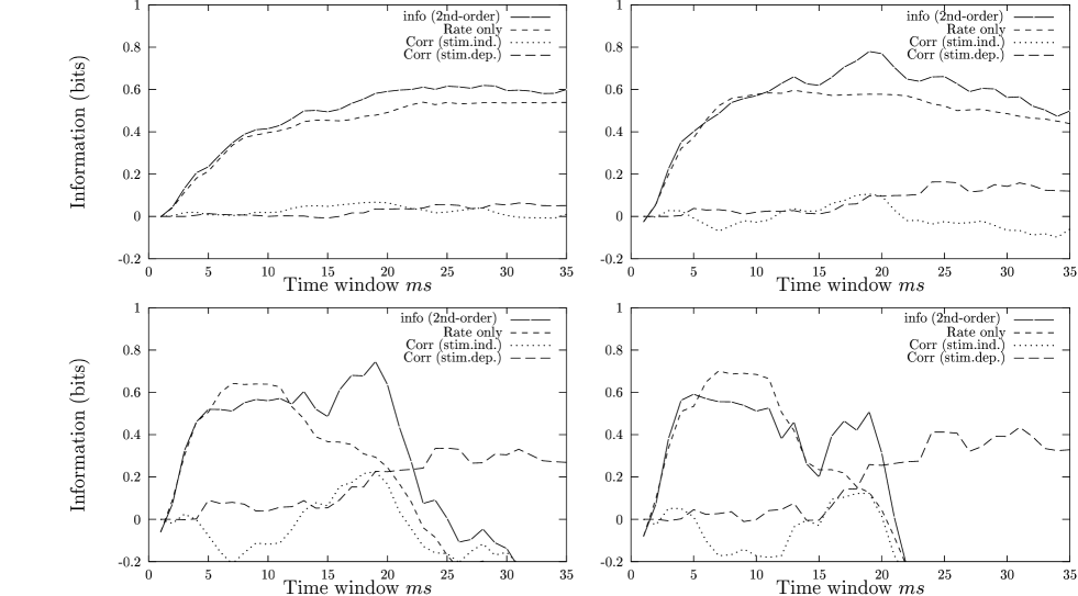
Figure 4: The short time limit expansion breaks down sooner when the larger population is considered. Cells in rat somatosensory barrel cortex for $2$ stimulus sites. Components of the transmitted information (see text for details) with $3$ (top, left), $6$ (top, right), $9$ (bottom, left) and $12$ cells (bottom, right). The initial slope (i.e. $I_{t}$) is roughly proportional to the number of cells. The effects of the second order terms, quadratic in $t$, are visible over the brief times between the linear regime and the break-down of the expansion. Information is estimated taking into account finite sampling effects [22]. Time window starts $5ms$ after the stimulus onset.

In Fig. 4 we have plotted, for the same experiment, the values of the information and of single terms of the second order expansion discussed above. The full curve represents the information $I(t)$ up to the second order, i.e. $I(t)=t\;I_{t}+{t^{2}\over 2}\;I_{tt}$ The short dashed curve is the sum $I_{t}t+\frac{1}{2}I_{tt}^{(1)}t^{2}$, i.e. the rate only contribution, as it depends only on average firing rates, $\overline{r}_{i}(s)$. The dotted line represents $\frac{1}{2}I_{tt}^{(2)}t^{2}$, i.e. the contribution of correlations to information even if they are stimulus independent. The last second-order term, $\frac{1}{2}I_{tt}^{(3)}t^{2}$, is non-zero only if the correlations are stimulus dependent. We expect $I_{t}$ to grow linearly with the number of cells, and in fact the slope of the total information (full curve in Fig. 4) increases linearly, at least for the short time interval before the second derivative starts to bend it down. As mentioned above, the number of second order terms grows as $C^{2}$, causing the range of validity of the expansion up to second order to decrease with the number of cells, as evident in Fig. 4. Note that, in general, as the number of cells increases one would expect an increase in the information they conveyed, which is not what one observes in Fig. 4, except in the brief initial linear regime. This is an indication of the failure of the second order expansion, which for $12$ cells appears to break down after little more than $5ms$ from the response onset.

5 Conclusions

The contribution of pairwise correlations to the total information conveyed by the activity of an ensemble of cells can be quantified by introducing a Taylor expansion of the information transmitted over cumulative time intervals, and calculating its terms up to second order. The range of validity of the expansion depends on the overall magnitude of second order terms with respect to first order ones. We have shown, by considering a model with ‘small’ random correlations in a large ensembles, that for times $t\simeq{\rm ISI}$ (inter-spike interval), the expansion would already begin to break down. The overall contribution of first order terms is in fact of order $C$, while second order ones are of order $-C^{2}\left<\nu^{2}\right>_{C}$ (redundancy) and $C^{2}\left<\delta\gamma^{2}\right>_{C}$ (synergy). These ‘random’ redundancy and synergy contributions will normally be substantial, unless a specific mechanism minimizes the values of $\left<\nu^{2}\right>_{C}$ and $\left<\delta\gamma^{2}\right>_{C}$ well below order $1/C$.

Further, data from the somatosensory cortex of the rat indicate that the assumption of ‘small’ correlations may be far too optimistic in the real brain situation; the expansion may then break down even sooner, although one should consider that the rat somatosensory cortex is a “fast” system, with short-latency responses and high instantaneous firing rates.

Our data show (see Fig. 4) that the range of validity of the second-order expansion decreases approximatively as $1/C$. The length of the time interval over which the expansion is valid is roughly $10-15ms$ for $9$ or $12$ cells, in agreement with Panzeri and Schultz [24]. They have found, analyzing a large amount of cells recorded from the somatosensory barrel cortex of an adult rat, that for single cells the expansion works well up to $100ms$. In its range of validity this expansion constitutes an efficient tool for measuring information even in the presence of limited sampling of data, when a direct approach using the full Shannon formula, Eq.(1), turns out to be impossible [17]. When its limits are respected, the expansion can be used to address fundamental questions, such as extra information in timing and the relevance of correlations contribution.

It is important that if second order terms are comparable in size to first order terms, all successive orders in the expansion are also likely to be relevant. The breakdown of the expansion is then not merely a failure of the mathematical formalism, but an indication that this particular attempt to quantify, in absolute terms, the information conveyed by a large ensemble is intrinsically ill-posed in that time range. There might be other expansions, or other ways to measure mutual information e.g. the reconstruction method [25], that lead to better results.

A pessimistic conclusion is then that the expansion should be applied only to very brief times, of the order of $t\approx{\rm ISI}/C$. In this range the information rates of different cells add up independently, even if cells are highly correlated, but the total information conveyed, no matter how large the ensemble, remains of order 1 bit.

A more optimistic interpretation stresses the importance of considering information decoding along with information encoding. In this vein, not all pairwise correlations are taken into account on the same footing, and similarly not all correlations to higher orders; rather, appropriate models of neuronal decoding prescribe which variables can affect the activity of neurons downstream, and it is only a limited number of such variables that are included as corrections into the evaluation of the information conveyed by the ensembles. This embodies the assumption that real neurons may not be influenced by the information (and the synergy and redundancy) encoded in a multitude of variables that cannot be decoded. In an ideal world, it would be preferable to characterize the quantity of information present in population activity and to assume that the target neurons can conserve all such information. In real life, such an assumption does not seem to be justified, and considerable further work is now needed to explore different models of neuronal decoding, and their implementation in estimating information, in order to make full use of the potential offered by the availability of large scale multiple single-unit recording techniques.

References

- [1] E.T. Rolls, A. Treves and M.J. Tovée (1997) The representational capacity of the distributed encoding of information provided by populations of neurons in primate temporal visual cortex. Experimental Brain Research 114: 149-162.
- [2] E. Vaadia, I. Haalman, M. Abeles, H. Bergaman, Y. Prut, H. Slovin and A. Aertsen, (1995) Dynamics of neural interactions in monkey cortex in relation to behavioural events, Nature 373, 515-518.
- [3] R.C. deCharms, M.M. Merzenich, (1996), Primary cortical representation of sounds by the coordination of action potential, Nature 381, 610-613.
- [4] A. Riehle, S. Grun, M. Diesmann, A.M.H.J. Aertsen, (1997), Spike synchronization and rate modulation differentially involved in motor cortical function. Science 278, 1950-1953.
- [5] W. Singer, A.K. Engel, A.K. Kreiter, M.H.J. Munk, S. Neuenschwander and P. Roelfsema (1997) Neuronal assemblies: necessity, signature and detectability. Trends. Cogn. Sci. 1, 252-261.
- [6] E.M. Maynard, N.G. Hatsopoulos, C.L. Ojakangas, B.D. Acuna, J.N. Sanes, R.A. Normann and J.P. Donoghue, (1999) Neuronal interactions improve cortical population coding of movement direction. J. Neurosci. 19 8083-8093.
- [7] T. J. Gawne, and B. J. Richmond, (1993) How independent are the messages carried by adjacent inferior temporal cortical neurons?, J. Neurosci. 13: 2758–2771.
- [8] E. Zohary, M.N. Shadlen and W.T. Newsome (1994), Correlated neuronal discharge rate and its implication for psychophysical performance, Nature 370, 140-143.
- [9] M.N. Shadlen, W.T. Newsome (1998) The variable discharge of cortical neurons: implications for connectivity, computation and coding, J. Neurosci. 18, 3870-3896.
- [10] D.R. Golledge, C.C. Hildetag and M.J. Tovée (1996) A solution to the binding problem? Curr. Biol. 6, 1092-1095.
- [11] D.J. Amit, Is synchronization necessary and is it sufficient? Behav. Brain Sci. 20, 683.
- [12] E.T. Rolls, A. Treves (1998) Neural networks and brain function, Oxford University Press.
- [13] C.E. Shannon, (1948), A mathematical theory of communication, AT&T Bell Lab. Tech. J. 27, 279-423.
- [14] R. Eckhorn and B. Pöpel (1974), Rigorous and extended application of information theory to the afferent visual system of the cat. I. Basic concept, Kybernetik, 16, 191-200.
- [15] L.M. Optican, B.J. Richmond (1987), Temporal encoding of two-dimensional patterns by single units in primate inferior temporal cortex. III. Information theoretic analysis. J. Neurophysiol. 76, 3986-3982.
- [16] F. Rieke, D. Warland, R.R. de Ruyter van Steveninck, W. Bialek, (1996), Spikes: exploring the neural code. Cambridge, MA: MIT Press.
- [17] S. Panzeri, S. R. Schultz, A. Treves, and E. T. Rolls. (1999) Correlations and the encoding of information in the nervous system. Proc. Roy. Soc. (London) B 266: 1001–1012.
- [18] L. Martignon, G. Deco, K. Laskey, M. Diamond, W. Freiwald, E. Vaadia, Neural Coding: Higher Order Temporal Patterns in the Neurostatics of Cell Assemblies, Neural Computation 12, 1-33.
- [19] W. E. Skaggs, B. L. McNaughton, M. A. Wilson, and C. A. Barnes, (1992). Quantification of what it is that hippocampal cell fires encodes, Soc. Neurosci. Abstr., p. 1216.
- [20] W. Bialek, F. Rieke, R.R. de Ruyter van Steveninck and D. Warland (1991) Reading a neural code. Science 252: 1854-1857.
- [21] A.M.H.J. Aertsen, G.L. Gerstein, M.K. Habib and G. Palm, (1989) Dynamics of neural firing correlation. J. Neurophysol. 61, 900-917.
- [22] S. Panzeri and A. Treves (1996) Analytical estimates of limited sampling biases in different information measures. Network 7: 87-107.
- [23] M.A. Lebedev, G. Mirabella, I. Erchova and M.E. Diamond (2000), Experience-dependent plasticity of rat barrel cortex: Redistribution of activity across barrel-columns. Cerebral Cortex 10: 23-31.
- [24] S. Panzeri and S. R. Schultz (2000) A unified approach to the study of temporal, correlational and rate coding. Neural Computation in press.
- [25] F. Rieke, D. Warland, R.R. de Ruyter van Steveninck and W. Bialek, (1999) Spikes, MIT Press.