Probing interactions in mesoscopic gold wires

Abstract

We have measured in gold wires the energy exchange rate between quasiparticles, the phase coherence time of quasiparticles and the resistance vs. temperature, in order to probe the interaction processes which are relevant at low temperatures. We find that the energy exchange rate is higher than expected from the theory of electron-electron interactions, and that it has a different energy dependence. The dephasing time is constant at temperatures between 8 K and 0.5 K, and it increases below 0.5 K. The magnetoresistance is negative at large field scales, and the resistance decreases logarithmically with increasing temperatures, indicating the presence of magnetic impurities, probably Fe. Whereas resistivity and phase coherence measurements can be attributed to magnetic impurities, the question is raised whether these magnetic impurities could also mediate energy exchanges between quasiparticles.

Several recent experiments have demonstrated that the low-energy properties of quasiparticles in metallic thin films are sample-dependent. On the one hand, the power-law increase of the phase-coherence time with decreasing temperature, predicted by the theory of electron-electron interactions in diffusive wires [1], has been observed in several experiments [2, 3]. The energy exchange rates between electrons was found to be in agreement with this theory in experiments on silver wires [4]. On the other hand, the dephasing rate of quasiparticles was found to saturate at low temperature in a series of gold wires [5], and the energy exchange rate between quasiparticles in copper wires to display an energy dependence different from the predicted one [6]. We present here measurements on gold samples, in which the energy exchange rates have the same energy dependence as was observed in copper and have a magnitude even higher. In order to investigate the origin of this effect, we have performed resistance measurements on samples fabricated similarly. The logarithmic dependence of the resistance, the negative magnetoresistance at large field and the temperature dependence of the phase coherence time, which is constant between $8~{}\mathrm{K}$ and $0.5~{}\mathrm{K}$ and increases at lower temperature, suggest the presence of magnetic impurities, which might mediate electron-electron interactions.

I Energy exchange rates

A Measurement set-up

In order to access the energy exchange rates among quasiparticles, we have measured the distribution function $f(E)$ in a stationary out-of-equilibrium set-up [6], described in Fig. 1. We consider a mesoscopic metallic wire placed between two ideal reservoirs. In the absence of interactions, the population of quasiparticles at a given energy interpolates linearly between the distribution functions in the contacts, leading, if $k_{B}T\ll eU,$ to a double-step-shaped distribution function. In the opposite “hot electron” regime, in which the typical interaction time is much shorter than the diffusion time $\tau_{D}=L^{2}/D,$ equilibrium is reached locally at each position along the wire: the energy distribution function $f(x,E)$ is a Fermi function (see dotted curves in Fig. 1). If heat is only carried out by electrons, the local temperature is $T_{\mathrm{eff}}(x)=\sqrt{T^{2}+x\left(1-x\right)U^{2}/\mathfrak{L}},$ where $\mathfrak{L}=\frac{\pi^{2}}{3}\left(\frac{k_{B}}{e}\right)^{2}$is the Lorenz number [7, 8]. Our experiments focus on the intermediate regime, in which interactions lead to a significant redistribution of the energy among quasiparticles, but not to a complete thermalization. The distribution function is obtained from the differential conductance $dI/dV\left(V\right)$ of a tunnel junction between the wire and superconducting electrodes [6, 9]. When the temperature of the superconductor lies well below the superconducting transition temperature, and if the density of states in the normal electrode wire is taken as energy independent on the probed energy range, the differential conductance of the junction is simply proportional to the convolution product of the density of states in the superconductor $n_{S}(E)=\left|E\right|/\sqrt{E^{2}-\Delta^{2}},$ with $\Delta$ the gap of the superconductor, and of the energy derivative of the distribution function in the wire, $\frac{\partial f(x,E)}{\partial E}:$

$$\frac{dI}{dV}\left(V\right)=\frac{-1}{R_{t}}\int n_{S}(eV-E)\frac{\partial f(x,E)}{\partial E}dE,$$ (1)

with $R_{t}$ the tunnel resistance of the junction.

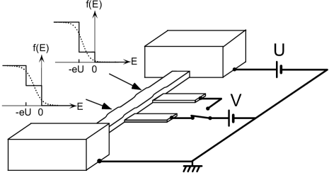
FIG. 1.: Experimental layout: a metallic wire of length $L$ is connected to large reservoir electrodes, biased at potentials $0$ and $U$. In absence of interaction, the distribution function at a distance $X=xL$ from the grounded electrode has an intermediate step $f\left(E\right)=1-x$ for energies between $-eU$ and $0$ (solid curves) (we assume $U>0$). When interactions are strong enough to thermalize electrons, the distribution function is a Fermi function (dotted curves). In the experiment, the distribution function is obtained from the differential conductance $dI/dV(V)$ of the tunnel junction formed by the wire and a superconducting electrode placed underneath.

B Samples

The samples were fabricated by deposition with an electron-gun, at several angles, through a PMMA suspended mask patterned using e-beam lithography. The substrate was thermally oxidized silicon, as in our experiments on Cu and Ag. We fabricated on the same chip two Au wires: wire #1, with length $L=1.55~{}\mu\mathrm{m,}$ and a single probe junction placed at $x=0.7$; and wire #2, with length $L=5~{}\mu\mathrm{m,}$ and two probe junctions, at $x=0.25$ and $x=0.5.\;$

We first deposited a $25~{}\mathrm{nm}$-thick aluminum film, which was then oxidized. This layer defines the superconducting probe electrodes. The wires and the pads were obtained by the subsequent evaporation from a 99.99% purity gold target, at a pressure of $10^{-6}~{}\mathrm{mb}$, at $1~{}\mathrm{nm/s}$. The thickness and width of the wires are $45~{}\mathrm{nm}$ and $165$ $\mathrm{nm}$. The electrodes at the ends of the wires are $500~{}\mathrm{nm}$-thick pads, with an area of about $1~{}\mathrm{mm}^{2}$. From the low temperature wire resistances $R_{1}=5.39~{}\Omega$ and $R_{2}=16.9~{}\Omega,$ we deduce from Einstein’s relation, assuming rectangular cross-sections, the diffusion constant $D=0.013~{}\mathrm{m}^{2}/\mathrm{s}$ and the diffusion times $\tau_{D1}=0.18~{}\mathrm{ns}$ and $\tau_{D2}=1.8~{}\mathrm{ns.}$ The samples were mounted in a copper box thermally anchored to the mixing chamber of a dilution refrigerator. Electrical connections were made through filtered coaxial lines [10].

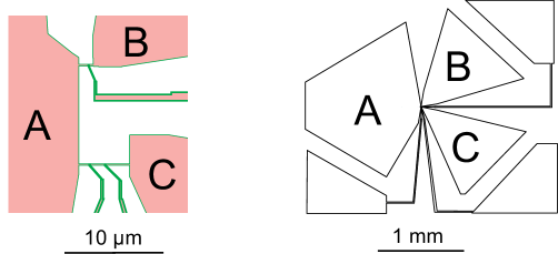
FIG. 2.: Micrometric scale (left) and large scale (right) shape of the sample. The wires are placed between pairs of large contact pads (wire #1 between A and B, wire #2 between A and C). Superconducting probe junctions are placed on wire #1 at $x=0.7$, on wire #2 at $x=0.25$ and $x=0.5$. The shape of the pads A, B, C has been designed to optimize the cooling of the reservoirs.

Measurements proceed as follows. In a first step, the voltage $U$ is set to zero. From the comparison of the measured differential conductance of the tunnel junctions with the calculated convolution product of the BCS density of states and of the derivative of a Fermi function at the temperature of the mixing chamber (see Eq. (1)), we deduce the gap of the superconductor ($\Delta\approx 0.2~{}\mathrm{mV}$) and the tunnel resistances [11] ($R_{t}=57~{}\mathrm{k\Omega}$ (wire #1), $28~{}\mathrm{k\Omega}$ and $30~{}\mathrm{k\Omega}$ (wire #2)). In a second step, the voltage $U$ is set to a dc value. From the differential conductance of the tunnel junctions, we deduce by numerical deconvolution the distribution functions in the wire at the position of the junctions, using Eq. (1) and the values of the gap and tunnel resistance determined in the first step.

C Distribution functions

We show in Fig. 3 the distribution functions measured with the three junctions at $U=0.1,$ $0.2,$ $0.3$ and $0.4$ $\mathrm{mV}$ [12].

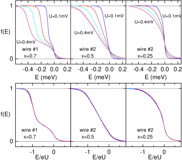
FIG. 3.: Measured distribution functions $f(E)$ on wire #1 (left panel) and wire #2 (central and right panel) for $U=0.1,~{}0.2,~{}0.3$ and $0.4~{}\mathrm{mV,}$ plotted as a function of $E$ (top) and $E/eU$ (bottom). The dotted line in the central panel is the prediction in the hot electron regime for $U=$ $0.4~{}\mathrm{mV.}$

As expected from the difference in the diffusion times, the distribution functions are much more rounded in wire #2 than in wire #1. The distribution function at the middle of wire #2 is close to the hot electron prediction, shown with a dotted line in the central panel for $U=0.4~{}\mathrm{mV.}$ However, the distribution functions measured on the same wire close to the left electrode (right panel) are clearly different from Fermi functions: they display a strong slope near $E=0,$ reminiscent of the Fermi step at this energy in the closest pad (A) which was grounded.

The larger the voltage $U,$ the wider the interval of energy in which $f$ varies from 1 to 0, as expected in both limiting regimes (see Fig. 1). In order to remove this dependence, we have replotted the same data in the bottom of Fig. 3, but with the reduced energy $E/eU$ on the horizontal axis. Remarkably, all scaled curves superimpose. This scaling property, which was also found in all the experiments on copper wires, is not generic: in experiments on silver wires, the slope of $f(E)$ at $E/eU=-0.5$ was found to increase with $U$ [4].

D Energy exchange kernel

The distribution function can be calculated by solving the stationary Boltzmann equation in the diffusive regime [13, 8]:

$$\frac{1}{\tau_{D}}\frac{\partial^{2}f\left(x,E\right)}{\partial x^{2}}+{\mathcal{I}}_{\mathrm{coll}}^{\mathrm{in}}\left(x,E,\left\{f\right\}\right)-{\mathcal{I}}_{\mathrm{coll}}^{\mathrm{out}}\left(x,E,\left\{f\right\}\right)=0$$ (2)

where ${\mathcal{I}}_{\mathrm{coll}}^{\mathrm{in}}\left(x,E,\left\{f\right\}\right)$ and ${\mathcal{I}}_{\mathrm{coll}}^{\mathrm{out}}\left(x,E,\left\{f\right\}\right)$ are the rates at which quasiparticles are scattered in and out of a state at energy $E$ by inelastic processes. The observation of the hot-electron regime in the middle of wire #2, with a temperature close to the expected one, indicates that the energy is mainly redistributed among the quasiparticles. In particular, phonon emission can be neglected. Assuming that the dominant inelastic process is a two-quasiparticle interaction which is local on the scale of variations of the distribution function,

$${\mathcal{I}}_{\mathrm{coll}}^{\mathrm{in}}\left(x,E,\left\{f\right\}\right)=\int{\mathrm{d}}\varepsilon{\mathrm{d}}E^{\prime}K\left(\varepsilon\right)f_{E+\varepsilon}^{x}(1-f_{E}^{x})f_{E^{\prime}}^{x}(1-f_{E^{{}^{\prime}}-\varepsilon}^{x})$$ (3)

where the shorthand $f_{E}^{x}$ stands for $f\left(x,E\right).$ The out-collision term ${\mathcal{I}}_{\mathrm{coll}}^{\mathrm{out}}$ has a similar form. The kernel function $K\left(\varepsilon\right)$ is proportional to the averaged squared interaction between two quasiparticles exchanging an energy $\varepsilon.$ We have neglected the possible dependence of $K(\varepsilon)$ on the energies of the initial and final states and on the position along the wire. The theory of electron-electron interactions in diffusive conductors in the $1\mathrm{D}$ regime [1] predicts $K\left(\varepsilon\right)\propto\varepsilon^{-3/2},$ a regime which was observed in silver wires [4]. In gold and copper wires, the scaling property implies, by a simple change of variables in Eq. (3), that $U^{2}K\left(\varepsilon\right)$ is a function of $\varepsilon/eU$ only [14]. If futhermore $K\left(\varepsilon\right)$ does not depend on $U,$ one obtains $K\left(\varepsilon\right)=\gamma/\varepsilon^{2},$ with $\gamma$ a typical interaction rate. We nevertheless tried to fit our data at $U=0.1~{}\mathrm{mV}$ with $K\left(\varepsilon\right)=\kappa/\varepsilon^{3/2}$, and obtained $\kappa=50~{}\mathrm{ns}^{-1}\mathrm{meV}^{-1/2}$, which is three orders of magnitude larger than the theoretical prediction $\kappa^{\mathrm{thy}}=(\hbar^{3/2}\nu S\pi\sqrt{D/2})^{-1}\approx 0.06~{}\mathrm{ns}^{-1}\mathrm{meV}^{-1/2},$ with $\nu$ the density of states in gold and $S$ the cross-section of the wire [15, 4]. Moreover, the shape of the distribution functions on wire #2 is not properly reproduced and the calculated curve for wire #1 at $U=0.4~{}\mathrm{mV}$ with the same parameter is significantly more rounded than the experimental data.

E Fits

Figure 4 shows the best fit of the data with $K\left(\varepsilon\right)=\gamma/\varepsilon^{2},$ obtained with $\gamma=8.9~{}\mathrm{ns}^{-1}$.

FIG. 4.: Symbols: measured distribution functions with $~{}U=0.1~{}\mathrm{mV}$ and (shifted vertically) $U=0.4~{}\mathrm{mV.}$ Solid lines: calculated distribution functions with the phenomenological kernel $K\left(\varepsilon\right)=\gamma/\varepsilon^{2}.$ Reservoirs are here assumed to be at $T=33~{}\mathrm{mK.}$

By construction, the scaling property of the data is exactly reproduced. Whereas the shape of the distribution functions on wire #2 is well accounted for, the experimental data on wire #1 are more rounded than we calculate. The opposite discrepancy was observed in experiments on $5$ $\mu\mathrm{m-}$long copper wires [16]. We attribute the strong rounding in the distribution functions on wire #1 to the large heating of the reservoirs associated with the low resistance of wire #1: at a given value of voltage $U,$ the heat power $P=U^{2}/R$ is the highest in the less-resistive wires. The solution of the heat equation in the contacts, assumed to have the shape of an angular sector, with angle $\theta$, and neglecting phonon emission, gives the reservoir temperature at the end of the wire [17]: $T=\sqrt{T_{0}^{2}+b^{2}U^{2}}.$ Here, $T_{0}$ is the temperature of the quasiparticles at a large distance $r_{\max}$ from the contact to the wire, and $b=\sqrt{\frac{1}{\theta\mathfrak{L}}\frac{R_{\Box}^{\mathrm{res}}}{R}\ln\frac{r_{\max}}{r_{\min}}},$ with $R_{\Box}^{\mathrm{res}}\approx 0.05~{}\Omega$ the sheet resistance of the reservoir, estimated from the resistivity of the wires and the thickness ratio of the wires and of the reservoirs, $r_{\max}\approx 1~{}\mathrm{mm}$ a typical equilibration length between electrons and phonons [18], and $r_{\min}$ the smallest radius for the radial approximation to be valid: $r_{\min}\approx w.$ In the experiment, the left contact (labelled A in Fig. 2), opens with an angle $\theta_{L}\approx 2.44\mathrm{~{}rad},$ whereas the two other contacts (B and C in Fig. 2) have a smaller angle: $\theta_{R}\approx 0.96\mathrm{~{}rad}.$ We have fitted the distribution functions separately from $U=0.005\ \mathrm{mV}$ to $U=0.5\ \mathrm{mV,}$ with the temperatures of the reservoirs as fit parameters. The results are shown in Fig. 5.

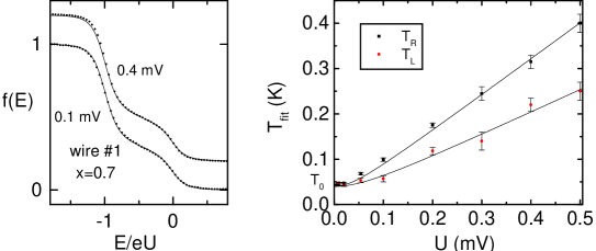
FIG. 5.: Left panel : distribution functions on wire #1 calculated with $K\left(\varepsilon\right)=\gamma/\varepsilon^{2}$ at $U=0.1\ \mathrm{mV}$ and $0.4\ \mathrm{mV,}$ the reservoirs temperatures being taken as fit parameters (solid lines). Symbols are data points. Right panel: symbols: temperatures of the right ($T_{R})$ and left ($T_{L}$) reservoirs obtained from the fits. Solid lines: reservoir heating model with $b$ as a free parameter.

At voltages below $20\ \mathrm{\mu V,}$ the fit temperature is nearly constant and identical in both reservoirs: $T_{0}=43~{}\mathrm{mK,}$ in reasonable agreement with the temperature $T=33~{}\mathrm{mK}$ indicated by the thermometer on the mixing chamber. At such low voltages, scaling is not obeyed since temperature produces a significant rounding of the steps and $eU/k_{B}T$ varies with $U.$ From the fit of the data on Fig. 5, we deduce $b_{L}=0.50~{}\mathrm{mK/\mu V}$ for the left contact, and $b_{R}=0.80~{}\mathrm{mK/\mu V}$ for the right contact. Theory gives $b_{R}/b_{L}=\sqrt{\theta_{L}/\theta_{R}}=1.60,$ in excellent agreement with the ratio found from the fits. Our estimated values of $b_{L}$ and $b_{R}$ are about a factor of 2 larger than those obtained from Fig. 5, possibly because the sheet resistance of the reservoirs is less than our estimate based on the electronic mean free path in the wire. At voltages larger than $50~{}\mu\mathrm{V}$, the temperature of the reservoirs is proportional to $U,$ leading to a scaling in the rounding of the steps. In contrast, we want to stress that the slope of the distribution function near $E/eU=-0.5$ cannot be explained by heating alone. The fits of the distribution functions in this regime, taking into account both $K\left(\varepsilon\right)=\gamma/\varepsilon^{2}$ (with $\gamma=8.9~{}\mathrm{ns}^{-1}$) and heating is shown on the left panel of Fig. 5. A consequence of reservoir heating is that the distribution functions are rounded at the scale of $\frac{k_{B}}{e}bU\approx U/15,$ and the sharp features that were observed on copper samples cannot not be resolved [16].

F Two-level systems

The distribution functions can also be well accounted for by a model in which quasiparticles are in local equilibrium with two-level systems distributed uniformly along the wire. The relevance of TLS on phase relaxation has recently been suggested by several authors [19, 20, 21]. Agreement is found if one assumes, in a simple model (described in [4]), that the quasiparticles are weakly coupled to the TLS with a density inversely proportional to the spacing $\varepsilon$ between the two levels. Such a density is obtained if the two-level systems are the two lowest energy levels in symmetric double-well potentials, and if the distribution of the barrier heights is uniform. In glasses the distribution of potential well asymmetries is usually taken as white [22], but one might argue that in metals, symmetric double-wells could result from crystalline symmetries  [23]. We note that a similar assumption is made in calculations based on a strong coupling to TLS [21].

II Resistance measurements

Complementary information on interactions was obtained from resistance measurements. We have fabricated long gold wires in the same deposition machine as for the energy relaxation experiment. To enhance adhesion of the Au film on the substrate, we used two different methods. For a first sample (Au1)  [3], we evaporated first $1~{}\mathrm{nm}$ of aluminum, and oxidized it. On a second sample (Au2), the surface of the sample was ion-milled just before gold deposition. A more complete set of data was taken on sample Au2, and we report only here the results on this sample. Its length, width and thickness are $L=271~{}\mu\mathrm{m,}$ $w=115~{}\mathrm{nm,}$ and $t=45~{}\mathrm{nm,}$ respectively. The low temperature resistance was $1125~{}\Omega.$ Assuming Einstein’s relation and a rectangular cross-section, we deduce the diffusion constant $D=0.016$ m²/s [24]. In another fabrication run conducted at Michigan State University, we have Joule evaporated another sample, called AuMSU, with very pure gold (99.9999%, i.e. $1~{}\mathrm{ppm}$ of impurities), with $L=176~{}\mu\mathrm{m,}$ $w=80~{}\mathrm{nm}$, $t=45~{}\mathrm{nm}$ and $D=0.016$ m²/s. All the samples were measured in the same top-loading dilution refrigerator.

A Resistance vs. temperature

We show in Fig. 6 the temperature dependence of the resistance for samples Au2 and AuMSU. The contribution of weak localization for Au2, smaller than $10^{-4}$ (see below), can be neglected. For AuMSU, this contribution, up to 3$\times 10^{-3}$ in $\delta R/R,$ has a well understood temperature dependence (see below), and was substracted. The contribution of electron-electron interactions to the resistivity, $\frac{\delta R_{ee}}{R}\approx 3.13\frac{R}{R_{K}}\frac{L_{T}}{L}=\frac{\alpha}{\sqrt{T}}$ [25], with $R_{K}=\frac{h}{e^{2}}$ and $L_{T}=\sqrt{\frac{\hbar D}{k_{B}T}},$ plotted as dotted lines in Fig. 6, accounts well for the data of AuMSU [26], where the fit parameter $\alpha=2.7\times 10^{-3}~{}K^{-1/2}$ is very close to the calculated value $\alpha^{\mathrm{thy}}=2.5\times 10^{-3}~{}K^{-1/2}.$ In contrast, the variations observed in Au2 are stronger and have a different temperature dependence.

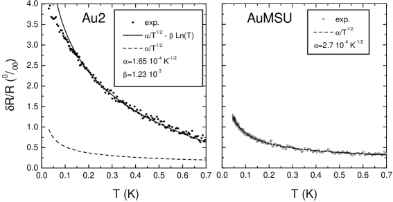
FIG. 6.: Relative variations of the resistance of sample Au2 and AuMSU as a function of temperature. The dotted line is the prediction of the theory of electron-electron interactions; the solid line on the left panel is a fit with an additional logarithmic term.

A good fit of the data can be obtained with: $\frac{\delta R}{R}=\frac{\delta R_{ee}}{R}-\beta\log T,$ with $\beta=1.23\times 10^{-3}.$ The logarithmic term is characteristic of the Kondo effect [27], and it was in particular studied in great detail in dilute alloys of Fe in Au [28, 29, 30, 31], where $\beta$ was found to be proportional to the Fe concentration and dependent on the cross section of the wire as well as on disorder. Assuming that the logarithmic dependence of the resistance of Au2 is due to Fe impurities, we get, by comparison with a sample with similar width, thickness and diffusion constant (AuFe2 in [31]), an impurity concentration $c\approx 55~{}\mathrm{ppm,}$ which is compatible with the purity of the gold source used for evaporation (99.99%, i.e. $100~{}\mathrm{ppm}$ of impurities) [32].

B Resistance vs. magnetic field - Phase coherence time

We present in the left panel of Fig. 7 the magnetoresistance of Au2 and AuMSU.  Around zero magnetic field, the resistance presents a dip, as expected from weak antilocalisation [1]. A large-scale negative magnetoresistance is found on Au2, which is similar to measurements performed on dilute alloys of Fe in Au [28, 31]. It can be attributed to the freezing of the magnetic moment of the impurities with the magnetic field [28]. In order to extract the phase coherence time from the magnetoresistance of Au2, we subtracted out the large scale magnetoresistance, which was, at each temperature, fitted with $\Delta R(B)/R=-r(T)(\sqrt{B_{0}^{2}+B^{2}}-B_{0}).$ The remaining magnetoresistance was then fitted with the predictions of the weak localization theory [1, 3]. In the right panel of Fig. 7, we show the phase coherence time $\tau_{\varphi}$ of samples Au1, Au2 and AuMSU as a function of temperature. Upon cooling, the phase coherence time of Au1 and Au2 remains unchanged from $8~{}\mathrm{K}$ to $0.5~{}\mathrm{K}$: $\tau_{\varphi}\approx 10~{}\mathrm{ps,}$ then it increases roughly as $1/T$. A simple interpretation of the very low value of $\tau_{\varphi}$ and of the desaturation below $0.5~{}\mathrm{K}$ is found by comparing with similar measurements performed on gold wires in which a small amount of iron was purposely introduced [28, 29, 5, 31]. The same behavior of $\tau_{\varphi}(T)$ was found in these experiments, and it was interpreted as an effect of spin-flip scattering by the impurities, the rate of which presents a maximum at the Kondo temperature of Fe in Au ($T_{K}\approx 0.3-1~{}\mathrm{K}$). The value $\tau_{\varphi}^{0}$ of $\tau_{\varphi}$ near the Kondo temperature was found to be roughly given by $\tau_{\varphi}^{0}\approx 0.25~{}\mathrm{ns/}c,$ with the concentration of impurities $c$ expressed in ppm (parts per million) [5, 31]. In this interpretation, $\tau_{\varphi}^{0}\approx 10~{}\mathrm{ps}$ is obtained for $c\approx 25~{}\mathrm{ppm.}$ This provides us with another estimation of $c$ which is of the same order of magnitude as what we deduced from the resistance vs. temperature measurements. Sample AuMSU does not show any magnetoresistance at large scale, and the phase coherence time presents no saturation down to $44~{}\mathrm{mK}$ (see Fig. 7). A good fit of the data could be obtained with the theoretical dependence [1] $\tau_{\phi}^{-1}=AT^{2/3}+BT^{3},$ with $A=0.9~{}\mathrm{ns}^{-1}\mathrm{K}^{-2/3}$ and $B=68~{}\mathrm{\mu s}^{-1}\mathrm{K}^{-3}.$ The theoretical value from the theory of electron-electron interactions is $A=0.5~{}\mathrm{ns}^{-1}\mathrm{K}^{-2/3}$ [25].

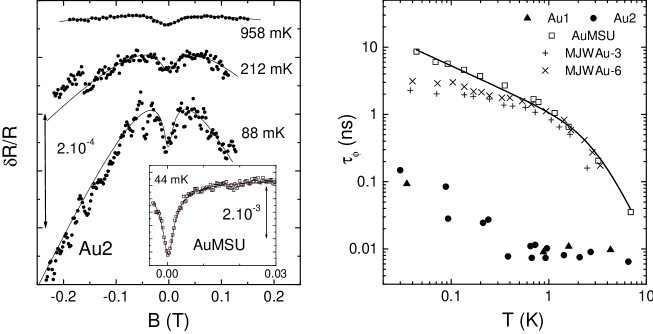
FIG. 7.: Left panel: Symbols: magnetoresistance of sample Au2 (vertical shifts between the curves taken at different temperatures are arbitrary) and of sample AuMSU (inset; note the difference in the scales). Solid curves: fit with the sum of the weak localisation expressions and (for Au2 only) of a phenomenological large scale contribution $-r(T)\sqrt{B_{0}^{2}+B^{2}}.$ Right panel: phase coherence time as a function of temperature, for samples Au1, Au2 and AuMSU. Solid line: fit of AuMSU with $\tau_{\phi}^{-1}=AT^{2/3}+BT^{3}.$ For reference, we have also plotted the data of two samples of Ref. [5] similar to AuMSU (MJW Au-3&6)

To allow for a comparison with the results of Mohanty et al., we have also plotted on the same figure the phase coherence time of samples Au-3 and Au-6 in [5], which have similar size and diffusion constants as AuMSU (Au-3: $w=100~{}\mathrm{nm}$, $t=35~{}\mathrm{nm}$ and $D=0.011$ m²/s; Au-6: $w=180~{}\mathrm{nm}$, $t=40~{}\mathrm{nm}$ and $D=0.016$ m²/s). It is clearly seen that our data do not display the saturation found in [5]. We had already found no saturation in measurements on silver wires [3], which were made from very pure (99.9999%) Ag. We suspect that energy exchanges in samples fabricated with very pure Au would be consistent with the theory of Ref. [1], as in very pure Ag [4], but this experiment remains to be performed. It is noteworthy that the low-temperature saturation of $\tau_{\phi}$ reported in Cu wires [3] was identically found in other samples obtained from 99.9999% Cu, supporting the hypothesis that surface oxide could play a major role in Cu [33].

III Can magnetic impurities mediate electron-electron interactions?

The data presented in section 2 provide strong evidence that some of the gold wires we have studied contain several tens of ppm of iron. The question arises as to whether the energy exchange measurements can also be explained by the presence of these magnetic impurities. Kaminski and Glazman [34] recently pointed out that $K(\varepsilon)\propto\varepsilon^{-2}$ is obtained in second order perturbation theory from the interaction of two quasiparticles with a magnetic impurity. The effective matrix element $M_{eff}$ of the second order process is proportional to $J^{2}/(E_{v}-E_{i}),$ where $J$ is the coupling parameter between the quasiparticles and the magnetic impurity and $E_{v}-E_{i}$ is the energy difference between the intermediate (virtual) state and the initial state. In the intermediate state, one quasiparticle is promoted to an energy state higher by $\varepsilon$ than the initial state, whereas the magnetic impurity has been reversed. One thus obtains $K(\varepsilon)\propto c\times\left|M_{eff}\right|^{2}=cJ^{4}/\varepsilon^{2},$ which has the energy dependence observed in the experiment, but the bare coupling parameter $J\approx 1/\nu\log(E_{F}/k_{B}T_{K})$ is too small. If one assumes that we have Fe impurities in Au, $k_{B}T_{K}\approx 50~{}\mu\mathrm{eV}$ is of the order of the energies probed in the energy exchange experiment, and the coupling constant is expected to be renormalised by the Kondo effect. This effect has been treated in [34], and the proposed expression $K(\varepsilon)=\frac{\pi}{2}\frac{c}{\hbar\nu}S(S+1)\log^{-4}(\frac{eU}{T_{K}})\frac{1}{\varepsilon^{2}},$ has now the right order of magnitude but too strong a $U$-dependence. Further work is clearly needed to clarify this issue.

REFERENCES

- [1] For a review, see B.L. Altshuler and A.G. Aronov, in Electron-Electron Interactions in Disordered Systems, Ed. A.L. Efros and M. Pollak, Elsevier Science Publishers B.V. (1985).
- [2] S. Wind, M.J. Rooks, V. Chandrasekhar, and D.E. Prober, Phys. Rev. Lett. 57, 633 (1986); P.M. Echternach, M.E. Gershenson, H.M. Bozler, A.L. Bogdanov and B. Nilsson, Phys. Rev. B 48, 11516 (1993).
- [3] A.B. Gougam, F. Pierre, H. Pothier, D. Esteve, and N.O. Birge, J. Low Temp. Phys. 118, 447 (2000).
- [4] F. Pierre, H. Pothier, D. Esteve, and M. H. Devoret, J. Low Temp. Phys. 118, 437 (2000). The measurements in all Ag wires can be accounted for by the effect of electron-electron interactions together with phonon emission, which we had incorrectly neglected for the -long wires in this work. The predicted intensity of the electron-electron interaction [1, 15] was between 3 and 12 times smaller than the experimental determination.
- [5] P. Mohanty, E.M.Q. Jariwala and R.A. Webb, Phys. Rev. Lett. 78, 3366 (1997).
- [6] H. Pothier, S. Guéron, Norman O. Birge, D. Esteve, and M. H. Devoret, Phys. Rev. Lett. 79, 3490 (1997).
- [7] A. H. Steinbach, J. M. Martinis, and M. H. Devoret, Phys. Rev. Lett. 76, 3806 (1996).
- [8] V. I. Kozub and A. M. Rudin, Phys. Rev. B 52, 7853 (1995).
- [9] J. M. Rowell and D.C. Tsui, Phys. Rev. B 14, 2456 (1976).
- [10] D. Vion, P.F. Orfila, P. Joyez, D. Esteve, and M. H. Devoret, J. Appl. Phys. 77, 2519 (1995).
- [11] We generally find that the current voltage characteristic of the junction presents a small hysteresis at voltages , that we attribute to surface effects on the probe electrode. When applying a small magnetic field () perpendicularly to the surface of the chip, this singularity disappears. The magnetic field is kept at the same value during all the experiment.
- [12] At voltages larger than tunneling of hot electrons into the superconductor results in a reduction of the gap of the probe electrode.
- [13] K.E. Nagaev, Phys. Lett. A 169, 103 (1992); Phys. Rev. B 52, 4740 (1995).
- [14] H. Pothier, S. Guéron, Norman O. Birge, D. Esteve, and M. H. Devoret, Z. Phys. B 104, 178 (1997).
- [15] A. Kamenev and A. Andreev, Phys. Rev. B 60, 2218 (1999).
- [16] The distribution functions measured on several Cu wires displayed very sharp steps at energies and (F. Pierre, Thèse de l’Université Paris 6, 2000).
- [17] M. Henny, S. Oberholzer, C. Strunk, and C. Schönenberger, Phys. Rev. B 59, 2871 (1999).
- [18] M.L. Roukes, M.R. Freeman, R.S. Germain, R.C. Richardson, and M.B. Ketchen, Phys. Rev. Lett. 55, 422 (1985).
- [19] Y. Imry, H. Fukuyama and P. Schwab, Europhys. Lett. 47, 608 (1999).
- [20] A. Zawadowski, Jan von Delft, D. C. Ralph, Phys. Rev. Lett. 83, 2632 (1999).
- [21] J. Kroha, this volume.
- [22] P.W. Anderson, B.I. Halperin, and C.M. Varma, Philos. Mag. 25, 1 (1972); W.A. Phillips, J. Low Temp. Phys. 7, 351 (1972).
- [23] J. von Delft, D.C. Ralph, R.A. Buhrman, S.K. Upadhyay, R. N. Louie, A.W.W. Ludwig, and V. Ambegaokar, Ann. Phys. 263, 1 (1998).
- [24] A slightly higher value m2/s is obtained from the resistivity ratio
- [25] I. L. Aleiner, B. L. Altshuler and M. E. Gershenson, Waves in Random Media 9, 201 (1999).
- [26] The same agreement was obtained in measurements of Cu and Ag wires.
- [27] A.C. Hewson, The Kondo Problem to Heavy Fermions (Cambridge University Press, 1993).
- [28] M.A. Blachly and N. Giordano, Phys. Rev. B 51, 12537 (1995); N. Giordano, Phys. Rev. B 53, 2487 (1996).
- [29] R. P. Peters, G. Bergmann, and R. M. Mueller, Phys. Rev. Lett. 58, 1964 (1987).
- [30] V. Chandrasekhar, P. Santhanam, N. A. Penebre, R. A. Webb, H. Vloeberghs, C. Van Haesendonck, and Y. Bruynseraede, Phys. Rev. Lett. 72, 2053 (1994).
- [31] P. Mohanty and R. A. Webb, Phys. Rev. Lett. 84, 4481 (2000).
- [32] A Secondary Ions Mass Spectroscopy analysis on a sample fabricated similarly to Au1 and Au2 concluded that the concentration of iron was smaller than 100 ppm.
- [33] J. Vranken, C. Van Haesendonck, and Y. Bruynseraede, Phys. Rev. B 37, 8502 (1988).
- [34] A. Kaminski and L.I. Glazman, cond-mat/0010379.