Weak localization in disordered systems at the ballistic limit

Abstract

The weak localization (WL) contribution to the two-level correlation function, $R(\omega)$, is calculated for two-dimensional disordered conductors. Our analysis extends to the nondiffusive (ballistic) regime, where the elastic mean path is of order of the size of the system. In this regime the structure factor, $S(t)$, (the Fourier transform of $R(\omega)$) exhibits a singular behavior consisting of dips superimposed on a smooth positive background. The strongest dips appear at periods of the periodic orbits of the underlying clean system. Somewhat weaker singularities appear at times which are sums of periods of two such orbits. The results elucidate various aspects of the weak localization physics of ballistic chaotic systems.

I Introduction

Interference effects, arising from the interplay of phases accumulated along different paths, are particularly interesting in ballistic chaotic systems. It is due to the hierarchy of importance among the classical trajectories in these systems: Long trajectories exhibit a universal statistical behavior, while short ones constitute the dynamical fingerprints of the system. The stable (and therefore usually also the shorter) the orbit is the stronger is its signature. This signature appears both in the wave functions (the scar phenomenon[1]) as well as in the statistical properties of the energy spectrum of the system[2]. The purpose of this paper is to study the fingerprints of the classical periodic orbits on the nature of interference in chaotic systems.

Our best understanding of quantum interference is in disordered systems. In these systems interference may lead to localization of the particle in space[3]. If, however, the disorder is too weak to localize the particle, interference manifest itself as an increase in the return probability compared to the classical value. This effect, known as weak localization (WL), has been observed by measuring the magnetoresistance of metallic films[4].

Recent advances in nanostructure technology[5], opened the possibility of manufacturing clean mesoscopic systems – systems in which the elastic mean free path, $l$, is of order of the size of the system, $L$. It is natural to ask what is the analogue of WL in such ballistic systems?

Very little is known about this issue, mainly because of the failure of periodic orbit theory to provide a simple systematic procedure for calculating interference (i.e. WL) corrections[6]. This failure has been one of the main motivations for constructing the supersymmetric nonlinear $\sigma$-model of ballistic systems[7]. The hope was that this model will produce a WL expansion for ballistic systems analogous to that of disordered systems. However, it turned out that WL crucially depends on the regularization of the field integral, and only specific cases could be worked out[8]. These are the cases where the dynamics is still diffusive or dictated by random matrix theory (RMT)[9].

Usually one would choose to study the WL signature in transport properties, because they are naturally related to the experimental data. However, this choice will be inappropriate for our purpose for the following reason: WL (similar to localization) takes place on a certain manifold in phase space. For example, in disordered systems this manifold is the real space, while in a circular billiard with rough boundaries localization occurs in the angular momentum space[10]. In general chaotic systems there is no preferred basis, therefore, WL may appear on a complicated manifold in the phase space[11]. Yet, transport measurements dictate a preferred basis, and may totally miss the WL physics we seek to describe.

Nevertheless, interference effects manifest themselves also in the spectral properties of chaotic systems, which are independent of the choice of basis. Therefore, in this work we shall focus our attention on the WL contribution to the simplest nontrivial spectral quantity – the two-level correlation function:

$$R(\omega)=\Delta^{2}\left\langle\rho(\epsilon+\hbar\omega)\rho(\epsilon)\right\rangle-1.$$ (1)

Here $\rho(\epsilon)=\sum_{\alpha}\delta(\epsilon-\epsilon_{\alpha})$ is the density of states, $\Delta=1/\langle\rho\rangle$ is the mean spacing between neighboring energy levels, $\epsilon_{\alpha}$, and the averaging, $\langle\cdots\rangle$, is over the disorder configurations or the energy $\epsilon$.

To state our problem in this context, consider the density of states of quantum system with Hamiltonian having a classical chaotic counterpart. Gutzwiller’s trace formula [12] expresses the density of states, in the semiclassical limit, as a sum over the classical periodic orbits of the system:

$$\rho(\epsilon)\simeq\frac{1}{\Delta}+\sum_{p.o.}A_{p}e^{\frac{i}{\hbar}s_{p}(\epsilon)},$$ (2)

where $s_{p}(\epsilon)$ is the action of the $p$-th periodic orbit, and $A_{p}$ is the corresponding amplitude depending on the stability of the orbit and its period [12].

The traditional way of calculating correlators such as (1), within periodic orbit theory, is to use the so called diagonal approximation [13, 2]. In this approximation one

FIG. 1.: (a+b) An illustration of pairs of orbits contributing to the diagonal approximation: (a) an orbit with itself, (b) an orbit with its time reversed counterpart. (c) The eight-shaped periodic orbits associated with the WL contribution to $R(\omega)$ in diffusive systems.

replaces a double sum over periodic orbits (such as that obtained when substituting (2) in (1)) by a single sum:

$$\left\langle\sum_{pp^{\prime}}A_{p}A^{*}_{p^{\prime}}e^{\frac{i}{\hbar}\left[s_{p}(\epsilon+\hbar\omega)-s_{p^{\prime}}(\epsilon)\right]}\right\rangle\to\frac{2}{\beta}\sum_{p}|A_{p}|^{2}e^{i\omega\tau_{p}},$$ (3)

where $\tau_{p}=\partial s_{p}(\epsilon)/\partial\epsilon$ is the period of the $p$-th orbit. The rational behind the diagonal approximation is that the coherent contributions, at $\omega=0$, come from pairs of orbits $(p,p^{\prime})$ having precisely the same action. Thus one should pair orbits with themselves, $p=p^{\prime}$ (Fig. 1a), as well as with other orbits related by symmetries such as time reversal symmetry (Fig. 1b). In the absence of other spatial symmetries, $\beta$ in the above formula is one for systems with time reversal symmetry, and two for systems which do not have this symmetry.

The problem of WL in the context of the two-level correlation function can be formulated as: How can one improve on the diagonal approximation to include interference effects systematically?

In seeking for the solution of this problem it is natural to inquire about the situation in disordered systems where the systematic interference corrections to the diagonal approximation is the “weak localization” expansion. The diagrammatic picture of the WL correction to $R(\omega)$ suggests that the WL contribution is associated with pairs of periodic orbits crossing themselves at some point in space as shown in Fig. 1c[14]. Thus along one loop the two orbits propagate in the same direction, while along the other loop they are in opposite directions. However, such orbits exist only in the presence of a non-classical scattering potential, and do not have a direct analog in the periodic orbit theory.

Facing this difficulty, in this work, we study WL using disorder diagrammatics but far from the diffusive regime, i.e. when the elastic mean free path is of order of the size of the system. In this case, the disorder is sufficiently weak, and traces of the short periodic orbits of the underlying clean system are still significant.

We, thus, consider a system consisting of a particle confined to move on a two dimensional torus, in the landscape of a random potential, see Fig. 2. The Hamiltonian

FIG. 2.: (a) An illustration of the model used in this paper for calculating the WL effects in the ballistic limit. The system consists of a non-interacting electron gas on a torus with white noise potential. This potential is sufficiently weak, such that the elastic mean free path is of order of the size of the system. (b) An equivalent representation of the system as a square with periodic boundary conditions.

of the system is

$$H=\frac{{\bf p}^{2}}{2m}+V({\bf r}),$$ (4)

where ${\bf p}$ is the momentum of the particle, $m$ is its mass, and $V({\bf r})$ is a Gaussian random potential defined by

$$\langle V({\bf r})\rangle = 0,~{}~{}~{}~{}\mbox{and}~{}~{}~{}~{}~{}\langle V({\bf r})V({\bf r}^{\prime})\rangle=\frac{\hbar}{2\pi\nu\tau}\delta({\bf r}-{\bf r}^{\prime}).$$ (5)

Here, $\nu=1/\Delta L^{2}$ is the averaged density of states per unit area, and $\tau$ is the elastic mean free time for scattering on the potential. This system has been considered earlier by Altland and Gefen [15] and by Agam and Fishman [16], but only in the framework of the diagonal approximation.

In analyzing the results of the above model, it will be convenient to use the spectral structure factor defined as

$$S(t)=\frac{\hbar}{\Delta}\int_{-\infty}^{\infty}d\omega R(\omega)e^{-i\omega t}.$$ (6)

Using $S(t)$ one can relate the quantum spectral properties of the system to the behavior of its classical analog. In particular, $S(t)$ form a connection to the periodic orbits of the system: Substituting (3) in (6) one sees that, within the diagonal approximation, the structure factor takes the form of a sum over peaks located at times which equal to the periods of the classical periodic orbits:

$$S(t)\simeq\frac{2h\Delta}{\beta}\sum_{p}|A_{p}|^{2}\delta(t-\tau_{p}).$$ (7)

It has been noticed by Argaman et al.[17] that the right hand side of the above equation can be also interpreted as $|t|p(t)$, where $p(t)$ is the classical return probability at time $t$. The notion of return probability has been further developed by Chalker et al. to obtain a more accurate description of the structure factor for diffusive electrons[18].

A disorder potential usually erases the $\delta$-singularities of $S(t)$ associated with the classical orbits of the clean system. But, if it is sufficiently weak, it will leave traces of the them. Indeed, $S(t)$ calculated, in the diagonal approximation, for weak disorder, shows a series of peaks [16] (see inset of Fig. 3). The locations of these peaks

FIG. 3.: The structure factor of chaotic systems with time reversal symmetry. The solid line represents the results of random matrix theory. Magnified is the regime where perturbation theory applies and nonuniversal corrections, which are the main focus of this paper, are important. Here we depict only the results of the contribution of the “diagonal approximation”. The peaks, indicated by pairs of winding numbers, are the signatures of the periodic orbits of the clean system (see Fig. 4). Both, the Fermi velocity and the system size, $L$, are set to unity. The elastic mean free path, in these units, is 1/2. $t_{H}=2\pi\hbar/\Delta$ is the Heisenberg time.

along the time axis are precisely the periods of the orbits of the clean system. (These orbits are defined by pairs of winding numbers which count the times the trajectory winds around the torus in each direction, see Fig. 4.)

In view of the behavior shown in Fig. 3 and the results of disorder diagrammatics, one may naively speculate that the WL contribution to the structure factor adds up in a similar way. Namely it consists of a series of singularities located at periods of the eight-shaped orbits illustrated in Fig. 1c. One may also expect this contribution to be positive, as in diffusive systems, since it should reflect an increase in the return probability compared to the classical value (i.e. the diagonal approximation).

However, as we show here, this picture is inaccurate. Indeed, in the ballistic regime, some singularities do appear at times which can be interpreted as periods of eight-shaped orbits (Fig. 1c). But these contributions are rather weak. A large negative contribution comes from the original periodic orbits. It is superimposed on a smooth positive background which is not related to properties of the clean system. At certain cases the WL contribution to the structure factor can even become altogether negative. Thus, in ballistic systems, it does not have, necessarily, a definite sign.

To make the paper self-contained, we organized it as follows: In the next section we prepare the mathematical background for our derivation by reviewing the standard results of disorder diagrammatics in the diffusive limit. This way we set the basis for extending the diagrammatic approach to the ballistic regime. In section III we

FIG. 4.: Periodic orbits of a particle moving on a tours are defined by pairs of integer numbers $(n_{x},n_{y})$. These “winding numbers” count the number of times the trajectory winds around the torus in the $x$ and in the $y$ directions, respectively. Some particular examples are: (a) the orbit (0,1) with length $L$, (b) the orbit (1,1) of length $2^{\frac{1}{2}}L$, and (c) the orbit (1,2) of length $5^{\frac{1}{2}}L$.

derive our central formulae for the WL contribution to $R(\omega)$, and the structure factor, $S(t)$. In section IV, we analyze these results and derive an asymptotic expression for $S(t)$. Finally, we summarize and present our conclusions in Section V.

II Background

The purpose of this section is to lay the technical background, and set the nomenclature for the analysis which will be carried out in the forthcoming sections. We shall review the main ideas of disorder diagrammatic technique for diffusive systems[19], present the basic building blocks, discuss the approximations involved, and the limits of applicability. Finally, we summarize the results for the WL contribution to $R(\omega)$ within RMT framework, and for diffusive systems. These results will form a reference point for the analysis of $R(\omega)$ in the ballistic limit, which will be carried out in the next section.

The disorder diagrammatic approach for Hamiltonians of the type (4) is an efficient way of constructing the perturbation expansion, in the weak potential $V({\bf r})$, for quantities averaged over the disorder configurations. Examples of such quantities are $n$-point spectral correlation functions, the magnetic susceptibility, and various properties of the conductance of disordered metals.

This diagrammatic approach is a semiclassical approximation in which the ratio of the particle wave length, $\lambda_{F}$, to the elastic mean free path, $l$, is assumed to be small. Therefore, it takes the formal form of an asymptotic series in powers of $1/k_{F}l$, where $k_{F}=2\pi/\lambda_{F}$ is the Fermi wavenumber. Yet, usually there will be also non-perturbative contributions, which are important when trying to resolve features on the scale of the mean level spacing, $\Delta$, or over time scales longer than the Heisenberg time $t_{H}=2\pi\hbar/\Delta$. Therefore, the applicability range of disorder diagrammatic is also limited to times smaller than the Heisenberg time, and energies larger than the mean level spacing.

As a first example, consider the average of the retarded Green function:

FIG. 5.: Example of diagrams contributing to the average Green function, $G_{\epsilon}^{R}({\bf k})$ (represented by the bold line). Thin lines represent the free Green function (i.e. in the absence of disorder), and dashed lines represents impurity scatterers.

$$G^{R}_{\epsilon}({\bf k})=\left\langle\frac{1}{\epsilon+i\eta-\frac{\hbar^{2}{\bf k}^{2}}{2m}-V({\bf r})}\right\rangle.$$ (8)

Here $\langle\cdots\rangle$ denotes an averaging over the configurations of the disordered potential, $\eta$ is an infinitesimal positive number, and ${\bf p}$ is the particle momentum. Expanding the Green function in powers of $V({\bf r})$, and changing representation to momentum space yields

$$G^{R}_{\epsilon}({\bf k})=G^{R}_{0}(\epsilon,{\bf k})+G^{R}_{0}(\epsilon,{\bf k})\left\langle V_{0}\right\rangle G^{R}_{0}(\epsilon,{\bf k})+~{}~{}~{}~{}~{}$$ (9)

$$+\sum_{{\bf k^{\prime}}}G^{R}_{0}(\epsilon,{\bf k})G^{R}_{0}(\epsilon,{\bf k^{\prime}})G^{R}_{0}(\epsilon,{\bf k})\left\langle V_{\bf k-k^{\prime}}V_{\bf k^{\prime}-k}\right\rangle+...$$ (10)

where $V_{\bf q}=\frac{1}{L^{2}}\int d^{2}re^{\frac{i}{\hbar}{\bf q\cdot r}}V({\bf r})$ is the Fourier transform of the potential (5), and $G^{R}_{0}(\epsilon,{\bf k})=1/(\epsilon+i\eta-\frac{\hbar^{2}k^{2}}{2m})$ is the free Green function. Terms containing an odd number of $V$-s vanish upon averaging, while those having an even number are calculated by Wick’s theorem (since the potential $V$ is Gaussian). Thus the average is equal to the product of averages of all possible pairs, such as $\langle V_{\bf q}V_{-{\bf q}}\rangle$. The various terms of this expansion can be represented diagrammatically as shown in Fig. 5.

A partial summation of the infinite series of the diagrams in Fig. 5, is achieved using Dyson’s equation, and summation over the irreducible diagrams (those which cannot be separated into two disconnected diagrams by cutting one internal propagator line, e.g. (b) (d) and (e) in Fig. 5). Thus the averaged Green function satisfies the relation

$$G^{R}_{\epsilon}({\bf k})=G^{R}_{0}(\epsilon,{\bf k})+G^{R}_{\epsilon}({\bf k})\Sigma G^{R}_{0}(\epsilon,{\bf k}),$$ (11)

where $\Sigma$ is the self energy given by the sum over all irreducible diagrams, see Fig. 6. To the leading order in $1/k_{F}l$, $\Sigma$ is the contribution of the first diagram in Fig. 6b. Thus

$$\Sigma \simeq \sum_{{\bf q}}\left\langle V_{\bf q}V_{-{\bf q}}\right\rangle G_{0}(\epsilon,{\bf k}+{\bf q})$$ (12)

$$= \frac{\hbar\Delta}{2\pi\tau}\left[P.V.\left(\int d\xi\frac{\rho(\xi)}{\epsilon-\xi+i\eta}\right)-\frac{i\pi}{\Delta}\right],$$ (13)

where $P.V.$ denotes the principle value of the integral. The real part of $\Sigma$ can be absorbed into the definition of the reference energy $\epsilon$, thus the solution of Dyson’s equation (11) yields

FIG. 6.: (a) The diagrammatic representation of Dyson’s equation for the average Green function (11). The bold and thin lines represents the dressed and the bare Green functions, respectively. (b) The self energy, $\Sigma$, given as a sum of irreducible diagrams.

$$G^{R}_{\epsilon}({\bf k})=\frac{1}{\epsilon\!-\!\epsilon({\bf k})\!+\!\frac{i\hbar}{2\tau}},$$ (14)

where $\epsilon({\bf k})=(\hbar k)^{2}/2m$. Similarly, the average of the advanced Green function is given by $G^{A}_{\epsilon}({\bf k})=(G^{R}_{\epsilon}({\bf k}))^{*}$.

Consider, next, the probability of a particle to arrive to ${\bf r}^{\prime}$ in time $t$, when its initial state, $|{\bf r};\epsilon_{F}\rangle$, is a wave packet localized near ${\bf r}$. We assume that this wave packet is composed of eigenstates centered at the Fermi energy, $\epsilon_{F}$, and ranging over an energy band of width $\hbar/\tau$. In the semiclassical limit $\hbar/\tau\ll\epsilon_{F}$, these conditions imply that the particle velocity, $v_{F}$, is well defined, and the wave packet width is of order of the elastic mean free path, $l=v_{F}\tau$. The probability density for finding the particle at point ${\bf r}^{\prime}$ after time $t$ is given by $P({\bf r}^{\prime},{\bf r};t)=L^{2}|U({\bf r}^{\prime},{\bf r};t)|^{2}$ where $U({\bf r}^{\prime},{\bf r};t)=\langle{\bf r}^{\prime}|e^{-\frac{i}{\hbar}Ht}|{\bf r};\epsilon_{F}\rangle$ is the propagator of the system. Using the convolution theorem, one obtains

$$P({\bf r}^{\prime},{\bf r};t)=\hbar\int d\omega e^{-i\omega t}\int d\epsilon\tilde{\cal D}({\bf r}^{\prime},{\bf r};\omega)$$ (15)

where

$$\tilde{\cal D}({\bf r}^{\prime},{\bf r};\omega)=L^{2}\left\langle G^{R}({\bf r}^{\prime},{\bf r};\epsilon_{F}+\hbar\omega)G^{A}({\bf r},{\bf r}^{\prime};\epsilon_{F})\right\rangle,$$ (16)

and $G^{R}({\bf r}^{\prime},{\bf r};\epsilon)$ and $G^{A}({\bf r}^{\prime},{\bf r};\epsilon)$ are the exact Green functions of the system for particular realization of the disordered potential. Notice that under our assumptions, $\tilde{\cal D}({\bf r}^{\prime},{\bf r};\omega)$ weakly depends on $\epsilon$, therefore the integration over $\epsilon$ results in a factor of $\hbar/\tau$.

The diagrammatic expansion of $\tilde{\cal D}({\bf r}^{\prime},{\bf r};\omega)$ proceeds along the same lines described above. It is convenient to perform the calculation in Fourier space, i.e. for

$${\cal D}({\bf q},\omega)=\left(\frac{\hbar}{2\pi\nu\tau}\right)^{2}\frac{1}{L^{2}}\int d{\bf r}e^{i{\bf q}\cdot{\bf r}}\tilde{\cal D}({\bf r}^{\prime},{\bf r}^{\prime}+{\bf r};\omega).$$ (17)

The leading contribution to ${\cal D}({\bf q};\omega)$, known as the diffuson, is given by the set of diagrams shown in Fig. 7a. The Dyson equation summing this set of diagrams yields

$${\cal D}(\bf q,\omega) = \frac{\hbar}{2\pi\nu\tau}\frac{1}{1-\Pi(\omega,\bf q)},$$ (18)

where

FIG. 7.: The diagrams of the diffuson (a) and the Cooperon (b), and their interpretations as the contribution of pairs of classical orbits associated with the retarded and the advanced Green functions: (c) An orbit with itself (diffuson) and (d) an orbit with its time reversed counterpart (Cooperon).

$$\Pi(\omega,{\bf q}) = \frac{\hbar}{2\pi\nu\tau}\int\frac{d^{2}k}{(2\pi)^{2}}G^{R}_{\epsilon+\hbar\omega}({\bf k}+{\bf q})G^{A}_{\epsilon}({\bf k})$$ (19)

$$\!\!\!\!\!\!\!\!\!\!\!\!\!\!\!= \!\!\!\!\!\!\!\!\frac{\hbar}{2\pi\tau}\int\frac{d\xi d\theta}{2\pi}\frac{1}{\xi+\hbar\omega\!-\!\hbar v_{F}q\cos\theta\!+\!\frac{i\hbar}{2\tau}}\frac{1}{\xi\!-\!\frac{i\hbar}{2\tau}}.$$ (20)

To obtain the second line of the above formula, we have expanded $({\bf k}+{\bf q})^{2}$ to linear order in ${\bf q}$, and approximated $2{\bf k\cdot q}$ by $2k_{F}q\cos\theta$, where $k_{F}$ is Fermi wave number, and $\theta$ is the angle between the vectors ${\bf k}$ and ${\bf q}$. This approximation is valid when $q\ll k_{F}$.

In the diffusive limit, additional approximations can be made. Namely, one may use the small parameters

$$ql\ll 1~{}~{}~{}\mbox{and}~{}~{}~{}\omega\tau\ll 1,$$ (21)

to expand $\Pi(\omega,{\bf q})$ in $\omega\tau$, and $ql$. The result takes the form $\Pi(\omega,{\bf q})\simeq 1+i\omega\tau-Dq^{2}\tau$, where $D=l^{2}/2\tau$ is the diffusion constant, thus

$${\cal D}({\bf q},\omega)=\frac{\hbar}{2\pi\nu\tau}~{}\frac{1}{-i\omega\tau+Dq^{2}\tau}.$$ (22)

This formula shows that the diffuson is the kernel of the diffusion equation: $\partial n/\partial t=D\nabla^{2}n$, where $n({\bf r})$ is the density of particles in real space. The diffuson is, therefore, the classical mode of a disordered system in the limit of long time ($\omega\tau\ll 1$) and large spatial scale ( $ql\ll 1$).

It is instructive to relate the diffuson to classical orbits[20]. For this purpose we turn to calculate $D({\bf r},\omega)$ using the van-Vleck approximation for the Green functions. A comment is now in order. The use of the van-Vleck propagator for a system with a white noise potential is unjustified, since the scattering is not semiclassical. Therefore, here, we assume the disorder potential to be in the form of randomly located hard scatterers of size larger than the particle wave length. This potential is semiclassical, and produces diffusion on large scales of time and space.

The van-Vleck’s formula for the Green function, $G^{R,A}({\bf r^{\prime}},{\bf r};\epsilon)$ is expressed as a sum over the classical trajectories[21] from ${\bf r}$ to ${\bf r^{\prime}}$ with energy $\epsilon$:

$$\begin{array}[]{l}G^{R}({\bf r^{\prime}},{\bf r};\epsilon)\simeq\frac{1}{\sqrt{2\pi\hbar}}\sum_{\mu}B_{\mu}e^{\frac{i}{\hbar}s_{\mu}({\bf r^{\prime}},{\bf r};\epsilon)},\\ G^{A}({\bf r},{\bf r^{\prime}};\epsilon)\simeq\frac{1}{\sqrt{2\pi\hbar}}\sum_{\mu}B_{\mu}^{*}e^{-\frac{i}{\hbar}s_{\mu}({\bf r^{\prime}},{\bf r};\epsilon)}.\end{array}$$ (23)

Here $s_{\mu}({\bf r^{\prime}},{\bf r};\epsilon)$ is the classical action of the $\mu$-th trajectory, while $B_{\mu}$ is the corresponding amplitude which can

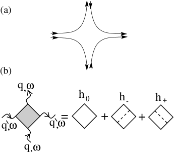
FIG. 8.: The Hikami box associated with the interaction between diffusons and Cooperons: (a) Its pictorial view in terms of “classical” trajectories. (b) Its diagrammatic expansion.

be interpreted as the square root of the classical probability to arrive to ${\bf r}^{\prime}$, after time $t$, starting from r. Substituting (23) in (16), yields $\tilde{\cal D}({\bf r}^{\prime},{\bf r};\omega)$ as a double sum over the classical trajectories from ${\bf r}$ to ${\bf r}^{\prime}$. Approximating the average of this double sum by the diagonal part, and substituting the result in (15) we obtain

$$P({\bf r}^{\prime},{\bf r},t)\simeq L^{2}\sum_{\mu}|B_{\mu}|^{2}\delta(t-\tau_{\mu}),$$ (24)

where $\tau_{\mu}$ is the time which takes for the particle to travel from ${\bf r}$ to ${\bf r}^{\prime}$ along the $\mu$-th trajectory. Using classical sum rules, one can sum over the classical trajectories[20]. The result for diffusive systems is that of the diagrammatic calculation. This implies that set of diagrams associated with the diffuson is equivalent to the diagonal approximation of pairs of orbits as shown in Fig. 7c.

In systems with time reversal symmetry there is an additional classical mode called Cooperon. It comes from the infinite sum over the maximally crossed diagrams shown in Fig. 7b. These diagrams are obtained by reversing the direction of the momentum in one of the Green function lines. The classical picture of the Cooperon is, therefore, that of an orbit paired with its time reversed counterpart as shown in Fig. 7d. It can be easily checked that the Cooperon has precisely the same analytical form of the diffuson.

The issue of WL, in the language of diagrammatics, is the interaction between diffuson and Coopron modes. Pictorially, this interaction is the switching between the directions of the momenta of two trajectories, as shown in Figs. 1c and 8a. The diagrammatic entity accounting for this switching is the Hikami box[22], see Fig. 8b. It is a function of the incoming and outgoing momenta and frequencies of the diffuson and the Cooperon. For the particular choice of momenta and frequencies shown in Fig. 8b one has $h({\bf q},{\bf q}^{\prime},\omega)=h_{0}+h_{-}+h_{+}$, where

$$h_{0} = \sum_{\bf k}G^{R}_{\epsilon+\hbar\omega}({\bf k})G^{R}_{\epsilon+\hbar\omega}({\bf k}\!-\!{\bf q}\!-\!{\bf q}^{\prime})G^{A}_{\epsilon}({\bf k}\!-\!{\bf q})G^{A}_{\epsilon}({\bf k}\!-\!{\bf q}^{\prime}),$$ (25)

$$h_{-} = \frac{\hbar\Delta}{2\pi\tau}h_{\frac{1}{2}}({\bf q},-{\bf q}^{\prime};\epsilon,\epsilon+\hbar\omega)h_{\frac{1}{2}}(-{\bf q},{\bf q}^{\prime};\epsilon,\epsilon+\hbar\omega)$$ (26)

$$h_{+} = \frac{\hbar\Delta}{2\pi\tau}h_{\frac{1}{2}}^{*}({\bf q},{\bf q}^{\prime};\epsilon+\hbar\omega,\epsilon)h_{\frac{1}{2}}^{*}(-{\bf q}^{\prime},-{\bf q};\epsilon+\hbar\omega,\epsilon),$$ (27)

while

$$h_{\frac{1}{2}}({\bf q},{\bf q}^{\prime};\epsilon,\epsilon^{\prime})=\sum_{\bf k}G^{A}_{\epsilon}({\bf k})G^{R}_{\epsilon^{\prime}}({\bf k}+{\bf q}^{\prime})G^{R}_{\epsilon^{\prime}}({\bf k}+{\bf q}).$$ (28)

The calculation of the above diagrams in the diffusive limit (21) (the corresponding integrals are provided in Appendix A), gives

$$h({\bf q},{\bf q}^{\prime},\omega) = \frac{4\pi\tau^{4}}{\hbar^{3}\Delta}[D(q^{2}+q^{\prime 2})-i\omega].$$ (29)

Having the basic ingredients of the disorder diagrammatics, we turn now to calculate the two-level correlation function defined by Eq. (1). Using the relation $\rho(\epsilon)=\mbox{Im}\left\{\mbox{Tr}G^{R}(\epsilon)\right\}/\pi$, we have

$$R(\omega)=\frac{\Delta^{2}}{2\pi^{2}} \left[\left\langle\mbox{Tr}G^{R}(\epsilon+\omega)\mbox{Tr}G^{A}(\epsilon)\right\rangle\right.$$ Re (30)

$$- \left.\left\langle\mbox{Tr}G^{R}(\epsilon+\omega)\right\rangle\left\langle\mbox{Tr}G^{A}(\epsilon)\right\rangle\right].$$ (31)

This formula can be used as a starting point for diagrammatic expansion. However, it produces a large number of diagrams. A convenient way of reducing this number is to express $R(\omega)$ in terms of a generating function which has a simpler diagrammatic expansion. This generating function, $F(\omega)$, has been found by Smith, Lerner and Altshuler[14]. It satisfies the relation:

$$R(\omega) = -\frac{\Delta^{2}}{2\pi^{2}\hbar^{2}}\frac{\partial^{2}}{\partial\omega^{2}}\mbox{Re}F(\omega),$$ (32)

and has the form of a free energy. The diagrammatic expansion of $F(\omega)$ can be loosely pictured as an expansion in the number of diffusons and Cooperons loops:

$$F(\omega)=F_{1}(\omega)+F_{2}(\omega)+F_{3}(\omega)+\cdots.$$ (33)

Thus, the leading term, $F_{1}(\omega)$, is the contribution of the one loop diagram (see Fig. 9), $F_{2}(\omega)$ is the two-loop contribution (plus two additional terms whose role is to remove the ultraviolet divergence in the first diagram), $F_{3}(\omega)$ comes from three-loop diagrams, etc[14]. In the periodic orbit picture, $F_{1}(\omega)$ is the contribution of orbits shown in Fig. 1a+b, while $F_{2}(\omega)$ is, in essence, the contribution of the eight-shape orbits illustrated in Fig. 1c.

The small parameter of the loop expansion (33) is $1/g$, where $g$ is the dimensionless conductance of the system. $g\propto t_{H}/t_{c}$ is the ratio of the Heisenberg time, $t_{H}=2\pi\hbar/\Delta$, to the classical relaxation time of particles in the system, $t_{c}$. In diffusive systems, $t_{c}=L^{2}/D$ (known as the Thouless time[23]) is the time which takes for a classical particle to diffuse across the system.

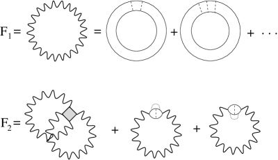
FIG. 9.: Diagrams of the free energy: $F_{1}(\omega)$ is the leading contribution associated with the diagonal approximation of periodic orbit theory. $F_{2}(\omega)$ is the WL contribution to the free energy associated with the eight-shaped orbits of Fig. 1c. Dashed impurity lines represent large momentum transfer, $k>1/l$, dotted lines represent small momentum transfer, $k<1/l$.

The form of the free energy (33) together with Eq. (32) induces a similar expansion for the two-level correlator:

$$R(\omega)=R_{1}(\omega)+R_{2}(\omega)+R_{3}(\omega)+\cdots,$$ (34)

where

$$R_{j}(\omega) = -\frac{\Delta^{2}}{2\pi^{2}\hbar^{2}}\frac{\partial^{2}}{\partial\omega^{2}}\mbox{Re}F_{j}(\omega),~{}~{}~{}~{}j=1,2,3\cdots.$$ (35)

Thus $R_{1}(\omega)$ is the result of diagonal approximation, $R_{2}(\omega)$ is the WL contribution, and additional terms give higher WL corrections.

The leading contribution to the two-level correlation function, $R_{1}(\omega)$, has been discussed extensively by Altshuler and Shklovskii[24]. It is straightforwardly calculated using (35). Taking into account the $1/n$ symmetry factor of the $n$ ladder diagram defining $F_{1}(\omega)$ (see Fig. 9) we obtain $F_{1}(\omega)=-\sum_{q}\ln(Dq^{2}\tau-i\omega\tau)$, where the diffusive approximation (21) has been assumed. Notice that although this sum does not converge, its second derivative with respect to $\omega$ does. Moreover, one can check that, in two dimensions, $R_{1}(\omega)=0$ for $\omega>0$. Thus the leading term in this case is the WL contribution[25].

In this paper we focus our attention on the WL contribution to $R(\omega)$ of two dimensional ballistic systems. As a reference point, however, it will be instructive to review results of RMT, and disorder diagrammatics in the diffusive limit. In both cases, our starting point is the diffusive form of the WL contribution to the free energy (obtained from the diagrams shown in Fig. 9):

$$F_{2}(\omega) = \frac{\Delta}{\hbar\pi}\sum_{{\bf q},{\bf q}^{\prime}}\frac{i\omega}{(Dq^{2}-i\omega)(Dq^{\prime 2}-i\omega)}.$$ (36)

The RMT result corresponds to the zero mode contribution (${\bf q}={\bf q}^{\prime}=0$) in the above sum, namely $F_{2}(\omega)\simeq-i\Delta/\hbar\pi\omega$. It is purely imaginary, therefore, Eq. (35) implies that $R_{2}(\omega)=0$ in the RMT limit. Since RMT accounts for the universal behavior of chaotic system, we conclude that $R_{2}(\omega)$ is a purely nonuniversal quantity.

Turning to the diffusive limit, we first note that the sum in (36) diverges logarithmically, even after differentiating twice with respect to $\omega$. Thus one has to introduce an upper cutoff on the momentum, which is usually taken to be $1/l$, where $l$ is the elastic mean free path. As will be shown in the next chapter this artificial cutoff can be avoided if the approximations (21) are not used in the calculations.

To evaluate $F_{2}$ in the regime $1/t_{c}\ll\omega\ll 1/\tau$, one can also use dimensional regularization[14]: Replacing the sums over ${\bf q}$ and ${\bf q}^{\prime}$ by integrals, and evaluating them in $d=2+\eta$ dimensions yields

$$F_{2}(\omega) = \frac{i\omega L^{4}\Delta}{\pi\hbar}\left[\int\frac{d^{d}q}{(2\pi)^{d}}\frac{1}{Dq^{2}-i\omega}\right]^{2}.$$ (37)

Changing variables from $q$ to $(iD/\omega)^{1/2}q$ and using the formula (see Appendix A)

$$\int\frac{d^{d}q}{1+q^{2}}=\pi^{d/2}\Gamma(1-\frac{d}{2}),$$ (38)

one arrives at

$$F_{2}(\omega) = \frac{iL^{4}\Delta}{\hbar\pi(4\pi D)^{2}}\left(\frac{-i}{4\pi D}\right)^{\eta}\Gamma^{2}(\frac{-\eta}{2})\omega^{1+\eta}.$$ (39)

$R_{2}(\omega)$ is now obtained by taking the second derivative with respect to $\omega$, as follows from Eq. (35). Thus using $\Gamma(1+\eta/2)\Gamma(-\eta/2)=\pi/\sin(-\eta\pi/2)$ we have

$$R_{2}(\omega) = -\frac{\Delta\pi(1+\eta)\eta\mbox{Re}[(-i\omega)^{\eta-1}]}{2\hbar g^{2}(4\pi D)^{\eta}\sin^{2}(-\eta\pi/2)\Gamma^{2}(1+\eta/2)},$$ (40)

where $g=4\pi^{2}\hbar D/L^{2}\Delta$ is the dimensionless conductance of the system. Finally we let $\eta\to 0$, and obtain

$$R(\omega)\simeq R_{2}(\omega)=-\frac{\Delta}{g^{2}\hbar\omega},\hskip 28.45274pt\frac{1}{t_{c}}\ll\omega\ll\frac{1}{\tau}.$$ (41)

Note that the domain of validity of the above formula vanishes in the ballistic limit since the classical relaxation time, $t_{c}$, is smaller or equal to the scattering time, $\tau$.

III Weak localization in the nondiffusive regime

In this section we calculate the WL contribution to the two-point correlator in the ballistic regime. By ballistic we refer to the situation in which the elastic mean free path, $l$, is of order of the size of the system $L$. To understand what kind of changes are needed in order to extend the diagrammatic calculation into the ballistic regime, recall that the diffusive approximation (21) corresponds to the leading order result in the small parameter $l/L$ (since $ql\ll 1$, $q$ is of order $1/L$, and $l\ll L$). In the ballistic regime this approximation cannot be used, and one has to evaluate integrals, such as (20) and (26), to all orders in $l/L$. Moreover, diagrams having a small number of impurity lines form the dominant contribution (unlike in the diffusive regime), therefore, possible cancellations among diagrams as well as double counting should be examined carefully. The outcome of this examination is that diffusons and Cooperons contributing to $F_{2}(\omega)$ should start from two impurity lines. Apart form this point, the WL contribution is given by the same diagrams shown in Fig. 9, but evaluated to all orders in $l/L$.

We begin by deriving an expression for the diffuson (starting from two impurity lines) in the ballistic regime. Dyson’s equation, in this case, yields

$${\cal D}({\bf q},\omega) = \frac{\hbar}{2\pi\nu\tau}\frac{\Pi(\omega,{\bf q})}{1-\Pi(\omega,{\bf q})},$$ (42)

where $\Pi(\omega,{\bf q})$ is the integral given by Eq. (20). To avoid the expansion in $ql$ and $\omega\tau$, here we first integrate over $\xi$ (by closing the contour in the complex plain), and then integrate over the angle, $\theta$, exactly. The result is $\Pi(\omega,{\bf q})=1/Q_{\omega}(q)$, where

$$Q_{\omega}(q) = \sqrt{(1-i\omega\tau)^{2}+(lq)^{2}}.$$ (43)

Thus the generalized formula for the diffuson is

$${\cal D}({\bf q},\omega) = \frac{\hbar}{2\pi\nu\tau}\frac{1}{Q_{\omega}(q)-1}.$$ (44)

A similar calculation for the Cooperon produces the same analytical expression.

The above formula holds both in the ballistic as well as the diffusive regime (21). It can be easily checked that an expansion of the denominator of Eq. (44) in $\omega\tau$ and $ql$, yields the result of the diffusive limit, (22).

The calculation of the Hikami box (Fig. 8b, Eq. 26), in the ballistic limit, follows along the same lines. Namely, one first integrates over the modulus of ${\bf k}$, and then the remaining angular integration is performed exactly. For example, after integration over the modulus of ${\bf k}$, Eq. (28) reduces to an integral of the from

$${\cal I}(x_{1},x_{2},\varphi)=\frac{1}{2\pi}\!\!\int_{0}^{2\pi}\!\!\!\!\frac{d\theta}{(1\!+\!x_{1}\cos\theta)(1\!+\!x_{2}\cos(\theta\!-\!\varphi))}.$$ (45)

The result of the integration over the angle $\theta$ (see Appendix A) is

$${\cal I}(x_{1},x_{2},\varphi)=\left(\frac{1}{y_{1}}+\frac{1}{y_{2}}\right)\frac{1}{1+y_{1}y_{2}-x_{1}x_{2}\cos(\varphi)}$$ (46)

where

FIG. 10.: The results for the WL contribution to the structure factor at various values of the ratio of the elastic mean free path, $l$, to the size of the system $L$. The WL effect, in this system, becomes stronger in two limits: (a) the diffusive regime, $\l\ll L$, where the particle approaches localization in real space, and (b) the ballistic limit, $l\gg L$, where the particle becomes localized in momentum space.

$$y_{i}=\sqrt{1-x_{i}^{2}},~{}~{}~{}~{}~{}~{}i=1,2.$$ (47)

With the help of this function, the various terms of the Hikami box (see Eq. (26) and Fig. 8b) take the form:

$$h_{\pm}=-\frac{2\pi\tau^{3}}{\hbar^{3}(1-i\omega\tau)^{4}\Delta}{\cal I}^{2}\left[\frac{ilq_{1}}{1-i\omega\tau},\frac{\pm ilq_{2}}{1-i\omega\tau},\varphi_{12}\right],$$ (48)

where $\varphi_{12}$ is the angle between ${\bf q}_{1}$ and ${\bf q}_{2}$, and

$$h_{0}=\frac{4\pi\tau^{3}(1\!-\!i\omega\tau)}{\hbar^{3}f_{1}^{2}f_{2}^{2}\Delta}{\cal I}\left[\left(\frac{lq_{1}}{\sqrt{2}f_{1}}\right)^{2}\!,\left(\frac{lq_{2}}{\sqrt{2}f_{2}}\right)^{2}\!,2\varphi_{12}\right],$$ (49)

where

$$f_{i}=\sqrt{(1-i\omega\tau)^{2}+(q_{i}l)^{2}/2}~{}~{}~{}~{}~{}~{}i=1,2.$$ (50)

Collecting the diagrams of $F_{2}(\omega)$ (Fig. 9) we obtain

$$F_{2}(\omega)=\frac{\hbar^{2}\!\Delta^{2}}{4\pi^{2}\!\tau^{2}}\!\sum_{1,2}\!{\cal D}_{1}{\cal D}_{2}\!\left[h_{0}\!+\!(h_{+}\!+\!h_{-})\!\left(\!\frac{1}{{\cal D}_{1}}\!+\!\frac{1}{{\cal D}_{2}}\!+\!1\!\right)\right],$$ (51)

where we use the notation

$${\cal D}_{i}=2\pi\nu\tau{\cal D}({\bf q}_{i},\omega)/\hbar,$$ (52)

and the sum is over the vectors ${\bf q}_{1}$ and ${\bf q}_{2}$. The periodic boundary conditions in our system imply that ${\bf q}_{i}\!=\!2\pi{\bf m}_{i}/L$ where ${\bf m}_{i}$ is an integer vector of two components.

The above formula is our central result. Performing the sum over momenta and substitution it in (35) gives the exact WL contribution to the two-level correlation function in the semiclassical limit. The applicability range

FIG. 11.: The weak localization contribution to the structure factor, in the ballistic regime, exhibits a singular behavior. The singularities are located at times which are linear combinations of periods of two orbits of the clean system (see Fig. 4). Here $t(n_{x},n_{y})=(n_{x}^{2}+n_{y}^{2})^{1/2}L/v_{F}$ denote the period of the periodic orbit defined by the pair of winding numbers $(n_{x},n_{y})$.

of our result goes beyond the diffusive limit, $l\ll L$, and includes the ballistic regime, $l\sim L$, as well. In contrast with the formula in the diffusive limit (Eq. 36), here the momenta sum converges, and there is no need to introduce an arbitrary cutoff or regularization. The results which will be shown below were obtained by performing the momenta sum numerically with cutoff chosen such that contribution of additional terms is of order of the numerical error.

In presenting our results it will be convenient to employ the spectral structure factor defined in Eq. (6). We denote by $S_{2}(t)$ the corresponding WL contribution,

$$S_{2}(t)=\frac{\hbar}{\Delta}\int d\omega R_{2}(\omega)e^{-i\omega t},$$ (53)

and rescale its magnitude by a factor of $2\pi^{3}g^{2}$, where $g\propto t_{H}/t_{c}$ is the dimensionless conductance of the system. Note that in the ballistic regime, the relaxation time, $t_{c}$, is no longer the diffusion time. It is approximately the traversal time across the system, $t_{c}=L/v_{F}$ where $v_{F}$ is the velocity of the particle, and $L$ is the size of the system. Therefore, from now on we define $g$ to be

$$g=\frac{\hbar v_{F}}{\Delta L}.$$ (54)

In Fig. 10 we plot $S_{2}(t)$, for various values of the ratio between the elastic mean free path and the size of the system. These values range from diffusive ($l/L=0.01$) to ballistic ($l/L=1.5$) dynamics. Several features of $S_{2}(t)$ are evident: First, the WL contribution appears only within a finite interval of time. It vanishes both at $t=0$ and when $t\to\infty$. Second, in both limits, $l\ll L$ and $l\gg L$, the WL contribution becomes strong. Third,

FIG. 12.: The convergence behavior of the momenta sum of the structure factor in the ballistic regime. The smooth part (dash-dotted) is determined by the zero mode, ${\bf q}_{1}={\bf q}_{2}=0$. The dashed line is the result of a sum over momenta within radius of $2.83\pi$. Higher $q$ terms build up singularities along the time axis as demonstrated by the solid line where the momenta sum extends to radius of $80\pi$.

in the ballistic regime, $l\sim L$, $S_{2}(t)$ exhibits a distinctive singular behavior consisting of a series of dips. These dips are located at times which are combinations of periods of the periodic orbits of the clean system. In Fig. 11 we depict $S_{2}(t)$ for $l=L/2$ and indicate the singularities with the corresponding combinations of periodic orbits.

IV Analysis

In analyzing the above results it is instructive to study, first, the convergence behavior of the momenta sum of the WL contribution. In Fig. 12 we depict the results for $S_{2}(t)$ calculated in the following approximations: The dash-dotted line is the contribution coming from the zero mode, ${\bf q}_{1}={\bf q}_{2}=0$. Clearly this mode dictates the gross behavior of $S_{2}(t)$. In particular, it determines the interval of time where WL is significant. The dashed line is the result obtained by taking into account the next lowest momentum modes, i.e. summing over ${\bf q}_{1}$ and ${\bf q}_{2}$ within the radius $q_{1},q_{2}\leq\sqrt{8}\pi$. In this approximation some additional features of $S_{2}(t)$ are resolved. The solid line is the result of the full momenta sum. Thus the singular behavior of the structure factor comes from the tail of the sum.

To obtain a simple analytic characterization of the WL contribution to the structure factor, we proceed in the following way. First, we derive a formula for the smooth part of $S_{2}(t)$ given by the contribution of the zeroth mode ${\bf q}_{1}={\bf q}_{2}=0$. This formula will give us the main parameters characterizing the WL contribution in the ballistic limit. Then, we evaluate the momenta sum in the asymptotic limit of large $\omega$. The result of this calculation provide the local behavior of $S_{2}(t)$ in the vicinity of the singularities.

To calculate the smooth part of $S_{2}(t)$, denoted hereinafter by $\bar{S}_{2}(t)$, we start by evaluating the zero mode contribution to $R_{2}(\omega)$. A straightforward calculation of the term ${\bf q}_{1}={\bf q}_{2}=0$ yields

$$R_{2}(\omega;q=0~{}\mbox{contrib.})=\frac{4\tau^{3}\Delta^{3}\left[5-54(\omega\tau)^{2}+21(\omega\tau)^{4}\right]}{\hbar^{3}\pi^{3}[1+(\omega\tau)^{2}]^{6}}.$$ (55)

Taking, now, the Fourier transform we obtain:

$$\bar{S}_{2}(t)=\frac{l^{2}}{12\pi^{2}g^{2}L^{2}}e^{-\tilde{t}}~{}\tilde{t}^{2}(\tilde{t}^{3}+3\tilde{t}^{2}+6\tilde{t}+6),$$ (56)

where $\tilde{t}=t/\tau$. We remark, here, that the above formula applies only in the ballistic regime, where the zeroth mode is dominant. In the diffusive systems, the zero mode contribution is negligible compared to that coming from the momenta sum in regime $1/L<q\ll 1/l$ (which is absent in the ballistic case).

Formula (56) allows one to characterize the major features of the WL contribution to the structure factor: The time $t^{*}$ where $\bar{S}_{2}(t)$ is maximal; its value at this point, $S_{2}^{*}$; and the width of the time interval where the WL effects are appreciable, $W^{*}$. The results are:

$$t^{*} = 4.24~{}\tau,$$ (57)

$$W^{*} = 2.46~{}\tau,$$ (58)

and

$$S_{2}^{*} = 0.353~{}\left(\frac{l}{Lg}\right)^{2}=0.353~{}\left(\frac{\tau\Delta}{\hbar}\right)^{2},$$ (59)

where the interval width is defined by $(W^{*})^{2}=\int dt\bar{S}_{2}(t)(t-t^{*})^{2}/\int dt\bar{S}_{2}(t)$. Thus WL effects, in the ballistic limit, are pronounced within a time interval of width $2.46\tau$ centered at $t=4.24\tau$, and the typical value of the WL contribution is proportional to $\tau^{2}$.

Note that these results are independent of the size of the system. Therefore the gross behavior of $S_{2}(t)$ is not influenced by the periodic orbits of the clean system. It is natural to ask what is the role the classical orbits of the system? As we show below, these orbits lead to the singular features decorating the smooth part of the structure factor $\bar{S}_{2}(t)$ as demonstrated in Fig. 12.

In analyzing this singular behavior, we first notice that its main part comes from large $\omega$ or equivalently large values of the momenta ${\bf q}_{1}$ and ${\bf q}_{2}$. Therefore, to calculate this contribution it is sufficient to approximate the discrete angular sum of $F_{2}(\omega)$ (over the phase between the vectors ${\bf q}_{1}$ and ${\bf q}_{2}$) by an integral. The small parameter of this approximation is $1/\omega\tau$. From (46) one finds that the angular average of the WL contribution to the free energy, denoted by $\bar{F}_{2}(\omega)$, is:

$$\bar{F}_{2}(\omega)=\frac{\tau\Delta}{\pi\hbar}\sum_{{\bf q}_{1},{\bf q}_{2}}\frac{A+B+C}{Q_{1}Q_{2}(Q_{1}+Q_{2})(Q_{1}-1)(Q_{2}-1)},$$ (60)

where

$$A=\frac{1}{1-i\omega\tau},~{}~{}~{}B=\frac{1-i\omega\tau}{Q_{1}Q_{2}},~{}~{}~{}C=-B(Q_{1}+Q_{2}),$$ (61)

and

$$Q_{i}=Q_{\omega}(q_{i}).$$ (62)

At asymptotically large values of $\omega\tau$ the leading contribution comes from $C$. This is evident once noticing that when $\omega\tau\to\infty$, $Q_{i}\to\omega\tau$, and therefore $A,B=O(\frac{1}{\omega\tau})$ whereas $C=O(1)$.

Next we apply the Poisson summation formula to convert the sum over ${\bf q}_{1}$ and ${\bf q}_{2}$ into an integral. The free energy is then expressed as

$$F_{2}(\omega)\simeq\bar{F}_{2}(\omega)=\sum_{{\bf m},{\bf n}}F_{2}^{({\bf m},{\bf n})},$$ (63)

where ${\bf m}$ and ${\bf n}$ are integer vectors. As will be shown below, these integer vectors are associated with winding numbers of the periodic orbits of the clean system. Each term in formula (63) is of the form

$$F_{2}^{({\bf m},{\bf n})}=-\frac{\tau\Delta L^{4}}{\pi\hbar}(1-i\omega\tau)K(m)K(n),$$ (64)

where

$$K(m)=\int_{0}^{\infty}\frac{dq}{2\pi}\frac{qJ_{0}(mqL)}{Q_{\omega}^{2}(q)(Q_{\omega}(q)-1)}.$$ (65)

Here $J_{0}(x)$ is the Bessel function of zero order, and $m=|{\bf m}|$ is the magnitude of the vector ${\bf m}$. For $m=0$ this integral yields

$$K(0)=\frac{1}{2\pi l^{2}(1-i\omega\tau)}+O\left(1/\omega^{2}\right).$$ (66)

For $m\neq 0$ the integral (65) can be calculated using the steepest descents method (see Appendix B), and in the large $m$ limit it gives

$$K(m)\sim-\frac{e^{3/2}}{\sqrt{72}\pi l^{2}}\frac{e^{-\frac{mL}{l}(1-i\omega\tau)}}{1-i\omega\tau}.$$ (67)

The above results imply the following form of the structure factor

$$S_{2}(t)\sim\bar{S}_{2}(t)+\sum_{{\bf n},{\bf m}}S_{2}^{({\bf n},{\bf m})}(t),$$ (68)

where

$$S_{2}^{({\bf n},{\bf m})}(t)=-B_{nm}\left(\frac{L}{gl}\right)^{2}\Theta[t-t_{nm}]~{}\tilde{t}^{2}e^{-\tilde{t}}$$ (69)

is the contribution associated with orbits characterized by the winding vectors ${\bf n}$ and ${\bf m}$. Here $\tilde{t}=t/\tau$, $t_{nm}=(n+m)L/v_{F}$, and $\Theta(x)$ is the step function. The amplitude of each contribution, $B_{nm}$, depends on the values ${\bf n}$ and ${\bf m}$. For cases where either ${\bf n}$ or ${\bf m}$ vanish, $B_{0m}=B_{n,0}\simeq e^{3/2}/12\sqrt{2}\pi^{4}$, while if $n$ and $m$ are large, $B_{nm}\simeq e^{3}/144\hbar^{2}\pi^{4}$.

Thus, $S_{2}(t)$ is composed of a smooth contribution (56) and a sequence of singular functions, of the form $-t^{2}e^{-(t-t_{mn})/\tau}\Theta(t-t_{mn})$, where $t_{mn}$ is the period of a composite orbit, i.e. the sum of periods of two periodic orbits of the clean system. Each singular contribution is negative, and its magnitude at time $t_{mn}$ is proportional to $t_{mn}^{2}e^{-t_{mn}/\tau}/l^{4}$. The contribution associated with single orbits (i.e. when either $n$ or $m$ vanish) is considerably larger than that of composite orbit (in which both $n$ and $m$ differ from zero). In any case, the singular contribution decreases exponentially in time , and as a power law in $1/l$ (when $L<l$). This behavior is indeed observed in Figs. 10, 11, and 12.

V Summary and concluding remarks

In this paper we have calculated the WL contributions to the two-level correlation function and its Fourier transform, the structure factor. These are the leading quantum interference effects which affect the spectral statistical properties of the system defined in (4).

Our theory generalize previous calculations of the WL contribution to the spectral statistics of diffusive systems[25] by extending them into the ballistic regime where the elastic mean free path, $l$, is of order of the size of the system, $L$. Here the disorder is weak enough to leave traces of the dynamics of the underlying clean system, which appear as singularities in the structure factor (Figs. 10, 11, and 12).

Our study has been focused on spectral rather than dynamical characteristics to avoid the problem of specifying the manifold on which WL takes place. Indeed Fig. 10 demonstrates that the WL contribution is pronounced in two limits. Panel (a) of Fig. 10 is a representative example of the results deep in the diffusive regime $l\ll L$, while panel (b) shows the typical behavior in the ballistic limit, $l=1.5L$. In both cases, the system approaches the strong localization limit, but the localization is of different nature. In the diffusive case, it is localization in real space [3], whereas in the ballistic case the localization is on a quasi-one-dimensional annulus in the momentum space. (This is evident once noticing that on clean torus, eigenstates are plain waves and therefore the particle is localized in momentum space.) In the latter case, it is suggestive that the effective dynamics is associated with Levy flights [26] rather than diffusion, since the disorder couples, predominantly, momentum states with degenerate eigenvalues, which may lie far away along the momentum annulus[27].

A simple semiclassical interpretation of our results, within periodic orbit theory, is not straightforward. The results, clearly, cannot be obtained from a diagonal approximation in which higher order $\hbar$ corrections are added to Gutzwiller’s trace formula (e.g. diffracting orbits, creeping orbits, etc. ). One can easily verified that such approximation yields only a positive contribution, in contrast with our results. This type of correction might explain the smooth positive part of the WL contribution, $\bar{S}_{2}(t)$. However, a correct analysis within periodic orbit theory must go beyond the diagonal approximation, and take into account pairing of orbits which are not related by symmetry, but have actions exponentially close one to the other (up to a constant phase, $\pi$, which is needed in order to explain the negative contribution of the periodic orbits). The fact that the WL contribution may become negative at certain times implies that the system exhibits anti-weak-localization at certain regions in phase space. This may be related to anti-scarring effects observed in wave functions of chaotic billiards[28].

Nevertheless, our work still elucidates several features of the leading WL effects in ballistic chaotic systems. First it shows that it appears within a finite interval of time; Second, it has a singular behavior associated with periodic orbits and linear combinations of periodic orbits; Third it can have different signs at different points in phase space.

These results have important consequences: First they show that the dominant contribution to the WL, in the ballistic regime, does not come from the eight-shaped orbits (Fig. 1c), as suggested by the diagrammatic picture. The main contribution comes from diffracting orbits (which are not related to the classical periodic orbits of the system), as well as from the original periodic orbits of the system. Moreover, the zero mode contribution, defining $\bar{S}_{2}(t)$, plays a dominant role here, while according to the results of the ballistic $\sigma$-model it should vanish (since the zero mode of the $\sigma$-model is identical to RMT). The apparent contradiction between our results and those of the ballistic $\sigma$-model is probably due to the fact that the ballistic $\sigma$-model does not account correctly for the return probability. This is also manifested by the so called “repetition problem” which is a small mismatch, associated with repetitions of periodic orbits, between the exact asymptotic results of periodic orbit theory and those of the ballistic $\sigma$-model. Ideas associated with memory effects in long range random potential[29] may be useful in resolving this problem.

Acknowledgment

It is our pleasure to thank Igor Aleiner, Alex Altland, Boris Altshuler, John Chalker, Igor Lerner, and Rob Smith for useful discussions. This work has been initiated at the “Extended Workshop on Disorder, Chaos and Interactions in Mesoscopic Systems” (Trieste, Aug. 98). We thank the I.C.T.P. and especially Volodya Kravtsov for the generous hospitality. This research was supported by THE ISRAEL SCIENCE FOUNDATION founded by The Israel Academy of Science and Humanities, and by The Herman Shapira foundation.

Appendix A. Useful integrals

In this appendix we calculate useful integrals frequently encountered when calculating diagrams which appear in this paper. The first type of such integrals appear when integrating products of retarded and advanced Green functions over the energy. The integral is of the form:

$$Y_{n,m}=\int_{-\infty}^{\infty}d\eta\left(\frac{1}{\eta+\frac{i}{2\tau}}\right)^{n}\left(\frac{1}{\eta-\frac{i}{2\tau}}\right)^{m},$$ (70)

where $n$ and $m$ are non-zero integers. Applying the Cauchy theorem, and using the fact that the coefficient $a_{-1}$ of a Laurent series, $\sum_{l}a_{-l}(z-z_{0})^{-l}$ of a function with an $n$-th order pole is $a_{-1}=\frac{1}{(n-1)!}\frac{d^{n-1}}{dz^{n-1}}\left[(z-z_{0})^{n}f(z)\right]_{z=z_{0}}$, one immediately gets

$$Y_{n,m}=\frac{2\pi(m+n-2)!~{}i^{m-n}{\tau}^{m+n-1}}{(n-1)!(m-1)!}.$$ (71)

The second type of integral appears when integrating over momenta in $d$ dimensions, e.g. in the calculation of the WL contribution to the free energy (37) in the diffusive limit. This family of integrals is of the form

$$I_{n,d}=\int\frac{d^{d}q}{(1+q^{2})^{n}},$$ (72)

where $n$ is an integer, $d$ is a real number, and $d^{d}q=d\Omega q^{d-1}$ denotes the measure in $d$ dimensions. Since the integrand is independent of the angles, the angular integral yields $\int d\Omega=d\pi^{d/2}/\Gamma(1+d/2)$. This formula should be understood as an analytic continuation of a function defined on an infinite set of integer values of $d$. Changing the integration variable to $x=q^{2}$ yields

$$I_{n,d}=\frac{\pi^{d/2}d}{2\Gamma(1+d/2)}\int_{0}^{\infty}dx\frac{x^{d/2-1}}{(1+x)^{n}}=~{}~{}~{}~{}~{}~{}~{}~{}~{}~{}~{}~{}~{}~{}~{}~{}$$ (73)

$$\frac{\pi^{\frac{d}{2}}d}{2\Gamma(1+\frac{d}{2})}\frac{(-1)^{n-1}\partial^{n-1}}{(n\!-\!1)!\partial\beta^{n-1}}\left.\int_{0}^{\infty}\!\!\!d\xi\int_{0}^{\infty}\!\!\!dxx^{\frac{d}{2}-1}e^{-\xi(x+\beta)}\right|_{\beta=1}.$$ (74)

Integrating over x, then changing the integration variable to $y=\xi\beta$, and integrating over $y$ we obtain

$$I_{n,d}=\frac{\pi^{d/2}\Gamma(d/2)\Gamma(1-d/2)(-1)^{n-1}}{\Gamma(n)\Gamma(1+d/2-n)}.$$ (75)

As the last step, we use the relation $\Gamma(x+1)=x\Gamma(x)$ to simplify the expression. The result is:

$$I_{n,d}=\pi^{d/2}\frac{\Gamma(n-d/2)}{\Gamma(n)}.$$ (76)

We turn now to evaluate the integral which appears when calculating diagrams in the ballistic limit, namely the integral defined by Eq. (45). It will be calculated in the regime $|x_{1}|,|x_{2}|<1$ (corresponding to the diffusive limit) and then analytically continued to the full complex plain. It is natural to substitute $z=e^{i\theta}$ which immediately transforms (45) into the contour integral

$$I(x_{1},x_{2},\varphi)=~{}~{}~{}~{}~{}~{}~{}~{}~{}~{}~{}~{}~{}~{}~{}~{}~{}~{}~{}~{}~{}~{}~{}~{}~{}~{}~{}~{}~{}~{}~{}~{}~{}~{}~{}~{}~{}~{}~{}~{}~{}~{}~{}~{}~{}~{}$$ (77)

$$~{}~{}~{}~{}~{}=\frac{-2i}{\pi x_{1}x_{2}}\!\oint_{|z|=1}\!\frac{zdz}{(z^{2}\!+\!\frac{2}{x_{1}}z\!+\!1)(z^{2}e^{-i\varphi}\!+\!\frac{2}{x_{2}}z\!+\!e^{i\varphi})}$$ (78)

$$~{}~{}~{}~{}~{}=\frac{-2ie^{i\varphi}}{\pi x_{1}x_{2}}\oint_{|z|=1}\frac{zdz}{(z-z_{1})(z-z_{2})(z-z_{3})(z-z_{4})}$$ (79)

where $z_{i}$ are

$$z_{1}=-\frac{1}{x_{1}}+\sqrt{\frac{1}{x_{1}^{2}}-1},~{}~{}~{}~{}~{}~{}~{}~{}~{}z_{2}=\frac{1}{z_{1}},$$ (80)

$$z_{3}=-\left(\frac{1}{x_{2}}+\sqrt{\frac{1}{x_{2}^{2}}-1}\right)e^{i\varphi},~{}~{}~{}~{}~{}~{}~{}z_{4}=\frac{e^{i2\varphi}}{z_{3}}.$$ (81)

Only the poles $z_{1}$ and $z_{3}$, which lie inside the unit circle, contribute to the integral. Thus using the residue theorem we get

$$I(x_{1},x_{2},\varphi)=\frac{4}{x_{1}x_{2}}\left[\frac{z_{1}}{(z_{1}-z_{2})(z_{1}-z_{3})(z_{1}-z_{4})}\right.$$ (82)

$$\left.+\frac{z_{3}}{(z_{3}-z_{1})(z_{3}-z_{2})(z_{3}-z_{4})}\right]~{}~{}~{}~{}~{}~{}~{}~{}~{}~{}~{}~{}~{}$$ (83)

Finally, we substitute (81) in (83) and arrived at (46).

Appendix B. Asymptotics of $K(m)$

In this appendix we evaluate the integral (65) in the asymptotic limit $m\gg 1$ and $\omega\tau\gg 1$. We begin by changing variables to $\eta=\frac{lq}{i+\omega\tau}$ and taking the leading term in $1/(i+\omega\tau)$. The result is

$$K(m) \simeq \frac{1}{2\pi l^{2}(i+\omega\tau)}\int\frac{\eta J_{0}(\frac{mL}{l}(i+\omega\tau)\eta)d\eta}{(\eta^{2}-1)^{\frac{3}{2}}}.$$ (84)

Being interested in the leading order expansion in $1/\omega\tau$, we further approximate the integral by substituting the asymptotic formula of the Bessel function: $J_{0}(x)\simeq\sqrt{\frac{2}{\pi x}}\cos(x-\pi/4)$ as $x\to\infty$. Representing the cosine as a sum of two exponents we arrive at:

FIG. 13.: The contour of integration for the asymptotic evaluation of $K(m)$. It is composed of steepest descent paths (a) and (b), connected by arcs, (c) and (d), which give vanishing contributions. The dashed lines represent cuts of the integrand in the complex plain (see Eq. 86)

.

$$K(m)\simeq\frac{1}{\sqrt{mL(2\pi l)^{3}(i+\omega\tau)^{3}}}~{}~{}~{}~{}~{}~{}~{}~{}~{}~{}~{}~{}$$ (85)

$$~{}~{}~{}~{}\times\sum_{\pm}\int\frac{\eta d\eta}{(\eta^{2}-1)^{\frac{3}{2}}}e^{\pm i\left[\frac{mL}{l}(i+\omega\tau)\eta-\frac{\pi}{4}\right]}.$$ (86)

The two terms in the above sum will be handled separately. Later, it will become clear, that the leading contribution to the integral comes from the plus-sign term. Therefore, for the time being, we ignore the term with the minus sign. Using the Cauchy theorem we can deform the contour of the integrals such that its direction near the edge at $\eta=0$ is a steepest descent direction. The contour is further deformed to follow steepest descent curves as illustrated in Fig. 13. Thus the contour consists of four segments: (a) from 0 to $i\infty/(1+i/\omega\tau)$, (b) the part surrounding the cut, (c) an arc connecting these two segments at infinity, and (d) an arc connecting the end of the (b) path and the original end point at $(\omega\tau-i)\infty.$

It is straightforward to check that the contribution from part (a) is of order $1/(\omega\tau)^{7/2}$. This contribution will turn out to be negligible compared to the one coming form segment (b). It is also clear that the contributions of arcs (c) and (d) vanish, when their distance form the origin approaches infinity. Thus we focus our attention on segment (b).

To evaluate the integral we exponentiate the pre-exponent factor in Eq. (86), and write the integral in the form

$$K(m)\simeq\frac{e^{-i\frac{\pi}{4}}}{\sqrt{mL(2\pi l)^{3}(i+\omega\tau)^{3}}}\int e^{A(\eta)}d\eta,$$ (87)

where

$$A(\eta)=i\frac{mL}{l}(i+\omega\tau)\eta-\frac{3}{2}\ln(\eta-1).$$ (88)

The steepest decent contour is found in the usual way: First, one takes the derivative of $A(\eta)$ with respect to $\eta$,

$$A^{\prime}(\eta)=i\frac{mL}{l}(i+\omega\tau)-3/2\frac{1}{\eta-1},$$ (89)

and find the saddle point $\eta^{*}$, satisfying $A^{\prime}(\eta^{*})=0$. The result is

$$\eta^{*}=u^{*}+iv^{*}=1-\frac{3l}{2mL(1-i\omega\tau)},$$ (90)

where $u^{*}$ and $v^{*}$ are real numbers. Second, one substitutes $\eta=(u-u^{*})+i(v-v^{*})$, where u and v are real, and solve for the curve which satisfies the condition

$$\mbox{Im}(A(\eta))=\mbox{Im}(A(\eta^{*}))$$ (91)

The formula for this curve is

$$\frac{v-\omega u}{u+\omega v-\frac{3}{2}}=\tan\frac{2}{3}(\omega u-v).$$ (92)

Rotating the axis as $x=v-\omega u$ and $y=u+\omega v$, one obtains

$$y=\frac{3}{2}-\frac{x}{\tan\frac{2}{3}x}.$$ (93)

This exact form shows that the contour can be indeed deformed as shown in Fig. 13. It also provides the possibility of constructing the full asymptotic expansion of the integral. However, in view of the approximations which already have been made, we are interested only in the leading term.

Thus, taking the quadratic approximation for the action: $A(\eta)\simeq A(\eta^{*})+\frac{1}{2}A^{\prime\prime}(\eta^{*})(\eta-\eta^{*})^{2}$, with

$$A^{\prime\prime}(\eta)=\frac{3}{2}\frac{1}{(\eta-1)^{2}},$$ (94)

and evaluating the resulting Gaussian integral we arrive at (67). Notice that the result is proportional to $1/\omega\tau$. Thus, the edge contribution (which is of order $1/(\omega\tau)^{7/2}$) can be indeed neglected. This calculation also shows that $A^{\prime\prime}(\eta^{*})\propto m^{2}$, and therefore the small parameter of this saddle point approximation is $1/m$.

The contribution of the second term in the sum (86), i.e the one with the minus sign, is calculated following along the same lines. However, it turns out that in this case the deformed contour does not pass through a saddle point, and the only contribution comes from the edge at $\eta=0$. It is, again, of order $1/(\omega\tau)^{7/2}$, and therefore can be neglected.

REFERENCES

- [1] E. J. Heller, Phys. Rev. Lett. 53, 1515 (1984).
- [2] M. V. Berry, Proc. Roy. Soc. London A 400, 229 (1985).
- [3] P. W. Anderson, Phys. Rev. 109 1492 (1958).
- [4] G. Bergmann, Phys. Rep. 107, 1 (1984).
- [5] See for example U. Sivan, F. P. Milliken, K. Milkove, S. Rishton, Y. Lee, J. M. Hong, V. Boegly, D. Kern and M. DeFranza, Europhys. Lett. 25, 605 (1994); C. M. Marcus, S. R. Patel, A. G. Huibers, S. M. Cronenwett, M. Switkes, I. H. Chan, R. M. Clarke, J. A. Folk, S. F. Godijn, K. Campman, and A. C. Gossard, Chaos Soliton Fract. 8, 1261 (1997); D. C. Ralph, C. T. Black, and M. Tinkham, Physica, 218V, 258 (1996); A. Yacoby, R. Schuster, and M. Heiblum, Phys. Rev. B 53, 9583 (1996); T. M. Fromhold, L. Eaves, F. W. Sheard, T. J. Foster, M. L. Leadbeater and P. C. Main, Phys. Rev. Lett. 72, 2608 (1994); G. Muller, G. S. Boebinger, H. Mathur, L. N. Pfeiffer, and K. W. West, Phys. Rev. Lett. 75, 2875 (1995); D. Goldhaber-Gordon, H. Shtrikman, D. Mahalu, D. Abusch-Magder, U. Meirav, and M. A. Kastner, Nature, 391, 156 (1998).
- [6] R. S. Whitney, I. V. Lerner, and R. A. Smith, Wave Random Media 9, 179 (1999).
- [7] B. A. Muzykantskii and D. E. Khmelnitskii, JETP Lett. 62, 76 (1995); A. V. Andreev, O. Agam, B. D. Simons, and B. L. Altshuler, Phys. Rev. Lett. 76, 3947 (1996).
- [8] I. L. Aleiner, and A. I. Larkin, Phys. Rev. B, 54, 14423, (1996); Phys. Rev. E, 55, R1243, (1997).
- [9] M. L. Mehta, Random Matrices and Statistical Theory of Energy Levels (Academic Press, New York, 1991).
- [10] F. Borgonovi, G. Casati, and B. Li, Phys. Rev. Lett. 77, 4744 (1996); K. M. Frahm and D. L. Shepelyansky, Phys. Rev. Lett. 78, 1440 (1997); K. M. Frahm, Phys. Rev. B, 55, R8626 (1997); K. M. Frahm and D. L. Shepelyansky, Phys. Rev. Lett. 79, 1833 (1997).
- [11] D. L. Shepelyansky, Phys. Rev. Lett. 56, 677 (1986).
- [12] M. C. Gutzwiller, Chaos in Classical and Quantum Mechanics (Springer, N.Y., 1990).
- [13] J. H. Hannay and A. M. Ozorio de Almeida, J. Phys. A 17, 3429 (1984).
- [14] R. A. Smith, I. V. Lerner, and B. L. Altshuler, Phys. Rev. B 58, 10343 (1998).
- [15] A. Altland and Y. Gefen, Phys. Rev. Lett. 71, 3339 (1993); Phys. Rev. B 51, 10671 (1995).
- [16] O. Agam and S. Fishman, Phys. Rev. Lett. 76, 726 (1996); J. Phys. A: Math. Gen. 29, 2013 (1996).
- [17] N. Argaman, Y. Imry, and U. Smilansky, Phys. Rev. B 47, 4440 (1993).
- [18] J. T. Chalker, I. V. Lerner, and R. A. Smith, Phys. Rev. Lett. 77, 554 (1996); J. Math. Phys. 37, 5061 (1996).
- [19] A. A. Abrikosov, L. P. Gor’kov, and I. E. Dzyaloshinski, Methods of Quantum Field Theory in Statistical Physics (Dover, New York, 1975).
- [20] This relation is derived in O. Agam Phys. Rev. E 61, 1285 (2000).
- [21] M. V. Berry and K.E. Mount, Rep. Phys. 35,315 (1972).
- [22] S. Hikami, Phys. Rev. B 24, 2671 (1981).
- [23] D. J. Thouless, Phys. Rep. 13 93 (1974).
- [24] B. L. Altshuler and B. I. Shklovskii, JETP 64, 127 (1986).
- [25] V. E. Kravtsov and I. V. Lerner, Phys. Rev. Lett. 74, 2563 (1995).
- [26] B. Mandelbrot, The Fractal Geometry in Nature (Freeman, San Francisco, 1982).
- [27] A similar situation appears in the Kepler billiard, see B. L. Altshuler and L. S. Levitov, Phys. Rep. 288, 487 (1997).
- [28] O. Agam and S. Fishman, Phys. Rev. Lett. 73, 806 (1994).
- [29] J. Wilke, A. D. Mirlin, D. G. Polyakov, F. Evers, and P. Wolfle, Phys. Rev. B 61, 13774 (2000).