Nonuniversal Correlations and Crossover Effects in the Bragg-Glass Phase of Impure Superconductors

Abstract

The structural correlation functions of a weakly disordered Abrikosov lattice are calculated in a functional RG-expansion in $d=4-\epsilon$ dimensions. It is shown, that in the asymptotic limit the Abrikosov lattice exhibits still quasi-long-range translational order described by a nonuniversal exponent $\eta_{\bf G}$ which depends on the ratio of the renormalized elastic constants $\kappa={c}_{66}/{c}_{11}$ of the flux line (FL) lattice. Our calculations clearly demonstrate three distinct scaling regimes corresponding to the Larkin, the random manifold and the asymptotic Bragg-glass regime. On a wide range of intermediate length scales the FL displacement correlation function increases as a power law with twice the manifold roughness exponent $\zeta_{\rm RM}(\kappa)$, which is also nonuniversal. Correlation functions in the asymptotic regime are calculated in their full anisotropic dependencies and various order parameters are examined. Our results, in particular the $\kappa$-dependency of the exponents, are in variance with those of the variational treatment with replica symmetry breaking which allows in principle an experimental discrimination between the two approaches.

]

I Introduction

The discovery of high-$T_{c}$ superconductors in 1986 by Bednorz and Müller [1] has led to a strongly renewed interest in the theory of superconductivity, both in the explanation of its microscopic origin [2] and in the application of the phenomenological theory on the determination of the phase diagram, of dissipation effects due to flux creep and related phenomena [3, 4].

Thermal fluctuations turned out to lead to a phase diagram drastically different from the mean-field prediction even in pure systems. This is due to the elevated transition temperatures as well as due to the pronounced layer structure of the high-$T_{c}$ materials. A liquid phase is now expected to separate the flux repulsing Meissner from the Abrikosov phase. In the latter the magnetic induction ${\bf B}$ enters the material in the form of quantized flux lines (FLs) which still form a triangular lattice. However, the upper critical field $H_{c_{2}}$ (where superconductivity disappears) is now strongly reduced with respect to its mean-field value and can be understood as resulting from a melting of the flux line lattice [3]. In fact there are several experiments on high–$T_{c}$ materials providing firm evidence that the Abrikosov lattice is melted over a significant region of the phase diagram [5, 6]. The field dependent melting line can be obtained from Lindeman’s criterion in conjunction with a detailed knowledge of the elastic properties of the lattice. In general, these properties have to be obtained by methods going beyond a simple continuum description [7]. Moreover, at present, it is not clear, whether the transition to the normal phase at high fields happens in these materials via one or two transitions.

It is well known that in addition to thermal fluctuations in type–II superconductors also the effect of disorder has to be taken into account since FLs have to be pinned in order to prevent dissipation from their motion under the influence of an external current. Therefore, understanding the interaction of vortices with quenched randomness in form of these defects is of especial importance.

A natural question arising in this context concerns the influence of randomness on the translational order of the lattice. This question was first considered by Larkin[8] who found from perturbation theory that randomly distributed pinning centers lead indeed to a destruction of the Abrikosov lattice. In particular, he obtained an exponential decay of the correlations of the order parameter for translational long range order $\Psi_{\bf G}({\bf r})=e^{i{\bf Gu}({\bf r})}$ on length scales larger than a disorder dependent Larkin length $L_{\xi}$. Here ${\bf G}$ and ${\bf u}$ denote a reciprocal lattice vector and the displacement field of the FL lattice, respectively, and ${\bf r}=({\bf x},z)$ is a 3-dimensional position vector.

This conclusion was in agreement with the more general observation of Imry and Ma, that quenched randomness coupled to a continuous symmetry order parameter destroys true long range order in less than four dimensions [9]. In this context the Imry-Ma argument played a similar role as the Mermin-Wagner theorem for pure system in two dimensions. In the latter case we know however, that the destruction of true long range order by thermal fluctuation contains still the possibility of topological order with an algebraic decay of correlations [10]. The intriguing possibility of a weak disorder phase with a topological order, which distinguishes it from the fully disordered phase at larger disorder strength, remained as an open question, and was discussed intensively in recent works.

As was first shown by Nattermann [11], in treating the interaction between FL lattice and disorder, it is crucial to keep the periodicity of this interaction under the transformation ${\bf u}\rightarrow{\bf u}+{\bf X}$, where ${\bf X}$ is a lattice vector of the Abrikosov lattice. This symmetry, which is abandoned in perturbation theory [8] and in the so-called manifold models [12], leads to a much slower, logarithmic increase of the elastic distortions, measured by the displacement correlation $B({\bf r})=\langle[{\bf u}({\bf r})-{\bf u}({\bf 0})]^{2}\rangle$ [11, 13, 14, 15]. If large dislocation loops can be neglected – as assumed in the above discussion – then the resulting phase is characterized by a structure factor with power-law singularities corresponding to a quasi-long-range ordered flux phase, the ”Bragg-glass” [14, 15], with algebraic decaying pair correlation function $C_{\bf G}({\bf r})=\langle\Psi_{\bf G}({\bf r})\Psi_{-\bf G}({\bf 0})\rangle$.

In three dimensions there is indeed strong theoretical [16, 17, 18, 19, 20, 21] and experimental [22] support of a phase transition from a fully disordered phase, where the occurrence of unbounded dislocation loops leads to an instability of the Bragg-glass, to a dislocation-free genuine glass phase at weak disorder.

The resulting power law decay of $C_{\bf G}({\bf r})$ in this Bragg-glass is reminiscent of the situation in pure 2D-crystals where in the solid phase $C_{\bf G}({\bf x_{\perp}})\sim|{\bf x_{\perp}}|^{-\eta_{{\bf G}}}$. This solid phase corresponds in fact to a line of critical points with $\eta_{{\bf G}}=TG^{2}(1+{\kappa}^{-1})/({4\pi}{\tilde{c}}_{11})$ and $\kappa={\tilde{c}}_{66}/{\tilde{c}}_{11}$. The ${\tilde{c}}_{ii}$ represent the renormalized elastic constants which have a finite temperature dependent value. At the melting temperature $T_{m}$ the exponent $\eta_{{\bf G}}$ reaches a non-universal value $\eta_{\bf G}=(Ga/4\pi)^{2}(1-{\kappa^{2}})$, which still depends on $\kappa(T_{m})$ [23].

Based on this rough analogy one could expect a similar non-universal behaviour for the Bragg-glass phase, although it is dominated by randomness and, therefore, by a zero temperature fixed point. But, in addition to the relevance of metastable states, the accuracy of earlier renormalization group approaches and variational techniques was particularly hampered by the complex elastic properties of the Abrikosov lattice. For instance, Giamarchi and Le Doussal [14, 15] calculated $C_{\bf G}({\bf x})$ using (i) a variational treatment for the triangular FL lattice and (ii) a functional renormalization group (FRG) in $d=4-\epsilon$ dimensions for a simplified model using a scalar displacement field $u$ with isotropic elasticity only. In both cases they found $C_{\bf G}({\bf x}_{\perp},0)\sim|{\bf x_{\perp}}|^{-\eta_{\bf G}}$ with a universal exponent ${\eta}_{\bf G_{0}}=A(4-d)$ with $A=1$ and $A=\pi^{2}/9\approx 1.1$ for the treatment (i) and (ii), respectively. Here ${\bf G}_{0}$ denotes one of the smallest reciprocal lattice vectors with $G_{0}a=4\pi/\sqrt{3}$, and $a=(2\phi_{0}/\sqrt{3}B)^{1/2}$ is the lattice spacing. To date, the question to which extent these results depend on the applied techniques and the simplifications of the considered models is not fully resolved.

In this paper, we systematically study the structural properties of the triangular Abrikosov lattice at weak disorder using a FRG method. Contrary to previous approaches, we explicitely take into account the triangular symmetry of the lattice and all of its elastic modes. We derive functional recursion relations for the correlation function of the random potential, which, in combination with a Fourier decomposition technique, allow us to extract detailed information about the collective wandering behaviour of the FLs. This transversal wandering can be characterized by the roughness exponent $\zeta$ controlling the displacement correlations via $B({\bf r})\sim|{\bf r}|^{2\zeta}$. Following the RG flow, three different scaling regimes can be clearly identified: On length scales smaller than the Larkin length, the FL are displaced by an amount smaller than the characteristic scale $\xi$ of the short range correlated random potential. Thus, Larkin’s perturbation theory holds with $\zeta=(4-d)/2$. Beyond this regime, but for line displacements still smaller than their distance $a>\xi$, one enters an intermediate regime with non-trivial roughness influenced by metastable states. Although this regime is similar to a single FL system, the complex elastic interactions of the lattice lead to a non-universal $\zeta$ depending on the ratio $c_{66}/c_{11}$ as reported here for the first time. Finally, on asymptotic scales, the FL displacement becomes larger than $a$, leading to the logarithmic roughness responsible for the quasi-order of the Bragg-glass phase. Using our Fourier technique to analyse the FRG flow equations, we were able to determine from the fixed point value $\Delta^{*}$ of the variance of the random potential the exponent $\eta_{\bf G}=\Delta^{*}(Ga)^{2}$ with sufficient accuracy to rule out universality. Instead, $\eta_{\bf G}$ depends also on the ratio $c_{66}/c_{11}$. The situation is therefore indeed qualitatively similar to that of 2D crystals at the melting temperature as speculated above. With the ratio $c_{66}/c_{11}$ depending in general on ${\bf B}$ and $T$, the observation of a field-dependent $\eta_{\bf G}$ would yield the opportunity to judge the validity of different approximation schemes under debate [24]. A brief description of our combination of FRG techniques and numerical calculations and these results appeared earlier [25].

The paper is organized as follows. First, we will introduce the model and examine its symmetries in Section 2. The derivation of the FRG flow equations and its numerical treatment is outlined in Section 3. A detailed discussion of the different scaling regimes and its correlation functions is given in Section 4. In this Section we also study correlation functions of various order parameters to obtain information beyond the translational order parameter as a signature of residual order at weak disorder. Experimental implications are presented briefly at the end of Section 4. Finally, in the last Section we summarize and discuss our central results. Lengthy computation is documented in the appendix.

II The Model

A The Hamiltonian

In order to examine the influence of disorder on the flux line lattice we employ the elastic description reviewed in Ref. [3]. The degrees of freedom are the positions of the flux lines $\{{\bf R}_{\bf X}(z)\}$ in the $(x,y)$-plane as a function of $z$, the direction of the external magnetic field, and ${\bf X}$, the lattice vectors of the perfect triangular Abrikosov lattice. To measure the disorder induced distortion of the flux lines, we introduce the displacements ${\bf u}_{\bf X}(z)={\bf R}_{\bf X}(z)-{\bf X}$ from the perfect lattice. Such a labelling with the perfect lattice positions is possible provided no dislocations are present in the system. The stability against dislocations has to be assured a posteriori, which gives a finite limit for the disorder strength [17, 16, 19, 18, 21, 20].

In an elastic continuum description the displacements are extended smoothly to a continuous function ${\bf u}_{\bf X}(z)\rightarrow{\bf u}({\bf r})$ with ${\bf r}=({\bf x},z)$. Symmetry reasons require three distinct elastic coefficients [26] and the energy cost of a distortion of the triangular line lattice is

$${\mathcal{H}}_{el} = {1\over 2}\int\!{\mbox{d}}^{2}x{\mbox{d}}z\left\{c_{11}\left(\nabla_{\perp}{\bf u}\right)^{2}+c_{66}\left(\nabla_{\perp}\times{\bf u}\right)^{2}+\right.$$ (2)

$$\hskip 62.59596pt\left.+c_{44}\left(\nabla_{z}{\bf u}\right)^{2}\right\}.$$

The elastic coefficients correspond to compression ($c_{11}$), shear ($c_{66}$) and tilt ($c_{44}$) of the lattice. The former two describe flux line interaction, while the tilt modulus contains both an interaction contribution and individual line tension. Such an elastic continuum description is valid as long as both displacements and their gradients vary slowly over lattice steps, which can be subsumed in the assumption of $L_{a}\gg a$. Here, $L_{a}$ is the positional correlations length, defined as the distance of two FLs whose mean displacements vary by the order of one lattice spacing $a$. In our context this is a condition on the weakness of disorder. Below we show that it can be easily satisfied by realistic impurity concentrations.

In wavenumber space, the elastic energy reads

$${\mathcal{H}}_{el} = {1\over 2}\int\limits_{\mbox{BZ}}\!{{{\mbox{d}}^{2}q_{\perp}{\mbox{d}}^{d-2}q_{z}}\over{(2\pi)^{d}}}{\bf u}({\bf q})\left({\mathcal{G}}^{-1}_{L}{\sf P}_{L}+{\mathcal{G}}^{-1}_{T}{\sf P}_{T}\right){\bf u}(-{\bf q}).$$ (3)

The integration runs over the Brillouin zone (BZ) and ${\sf P}_{L}^{\alpha\beta}=\frac{q_{\alpha}q_{\beta}}{q_{\perp}^{2}},\quad{\sf P}_{T}^{\alpha\beta}=1-\frac{q_{\alpha}q_{\beta}}{q_{\perp}^{2}}$ are projectors onto the longitudinal and transversal modes, respectively, with propagators

$${\mathcal{G}}^{-1}_{L} = c_{11}q_{\perp}^{2}+c_{44}q_{z}^{2}$$ (5)

$${\mathcal{G}}^{-1}_{T} = c_{66}q_{\perp}^{2}+c_{44}q_{z}^{2}.$$ (6)

This Fourier space formulation is more general than the model (2) since it both allows for wavenumber dependent elastic moduli and does not include the continuum limit as only wavevectors within the first Brillouin zone are included. The derivation of the elastic moduli from Ginzburg-Landau theory [27, 28] indeed gives $q$-dependent elastic constants on scales smaller than the London penetration length $\lambda$. However, this only leads to weakly renormalized constants on scales larger than $\lambda$. For the case of weak disorder considered here, we focus on the behaviour on scales far beyond $\lambda$ and may thus content ourselves with the local version (2). The coefficients $c_{ii}$ are understood to be the renormalized ones. In Eq. (3) we have formulated the model in general dimensions and extended the $z$-direction to a $d\!-\!2$ dimensional space. This will allow for an expansion around $d\!=\!4$ in the renormalization procedure below.

The interaction of flux lines with impurities competes with elasticity and tends to roughen the lattice. It is modelled by the coupling

$${\mathcal{H}}_{dis} = \int\!{\mbox{d}}^{d}\!r\>\rho_{\mbox{FLL}}({\bf r})V_{dis}({\bf r})$$ (7)

$$= \sum_{{\bf X}}\int\!{\mbox{d}}z^{d-2}\!\>V_{dis}\left({\bf X}+{\bf u}\left({\bf X},z\right),z\right)$$ (8)

of the flux line density

$$\rho_{\mbox{FLL}}({\bf r})=\sum_{{\bf X}}\delta\!\left({\bf x}-{\bf X}+{\bf u}\left({\bf X},z\right)\right)$$ (9)

to the disorder potential $V_{dis}({\bf r})$ with short range correlations on the scale $\xi=\max(\xi_{sc},\xi_{dis})$, where $\xi_{sc}$, $\xi_{dis}$ are the superconductor correlation length and the correlation length of disorder density fluctuations, respectively. The disorder potential is taken to be a random variable with Gaussian distribution. It is characterized by

$$\overline{V_{dis}({\bf r})}=0\>,\quad\overline{V_{dis}({\bf r})\,V_{dis}({\bf r}^{\prime})}=\Delta_{\xi}({\bf x}-{\bf x}^{\prime})\,\delta(z-z^{\prime}),$$ (10)

where $\Delta_{\xi}({\bf x})$ is a delta-function smeared out over a region of size $\xi$.

The continuum limit of Eq. (7) has to be taken with some care. Slow variations of the displacements do not suffice to allow a straightforward continuum limit. The potential $V_{dis}({\bf r})$ varies rapidly over lattice steps since $\xi\ll a$. Therefore, in the Hamiltonian rewritten using Poisson’s summation formula

$\displaystyle\sum_{{\bf X}}f({\bf X})=\int\!{\mbox{d}}^{2}\!xf({\bf x})[1+\sum_{{\bf G}\neq{\bf 0}}e^{i{\bf G}{\bf x}}]$

the terms corresponding to reciprocal lattice vectors ${\bf G}\neq{\bf 0}$ are important for the pinning energy and have to be considered adequately [11, 14].

$${\mathcal{H}}_{dis} = \rho_{0}\int\limits_{z}\!\!\!\int\limits_{{\bf x}}V_{dis}\left({\bf x}+{\bf u}\left({\bf x},z\right),z\right)[1+\sum_{{\bf G}\neq{\bf 0}}e^{i{\bf G}{\bf x}}]$$ (11)

$$= \rho_{0}\int\limits_{z}\!\!\!\int\limits_{\tilde{{\bf x}}}\left|\frac{\partial{\bf x}}{\partial\tilde{{\bf x}}}\right|V_{dis}(\tilde{{\bf x}},z)[1+\!\!\sum_{{\bf G}\neq{\bf 0}}e^{i{\bf G}[\tilde{{\bf x}}-\tilde{{\bf u}}(\tilde{{\bf x}},z)]}],$$ (12)

where $\rho_{0}=B/\Phi_{0}$ is the average FL density. In the last equation, we have substituted

$$\tilde{{\bf x}} \equiv {\bf x}+{\bf u}({\bf x},z)$$ (13)

$$\tilde{{\bf u}}(\tilde{{\bf x}},z) = \tilde{{\bf u}}({\bf x}+{\bf u}({\bf x},z),z)\equiv{\bf u}({\bf x},z).$$ (14)

With $\tilde{{\bf u}}(\tilde{{\bf x}})$, the displacement field is now written as a function of the actual position $\tilde{{\bf x}}$ of the flux lines rather than as a function of the perfect reference lattice coordinates ${\bf x}$. Such a relabelling is possible provided that $|\nabla u_{\alpha}|<1$, which is assured by the above assumption of $|\nabla u_{\alpha}|\backsimeq{a/L_{a}}\ll 1$.

The change of parameterization in Eq. (13) from $\{{\bf x},{\bf u}\}$ to $\{\tilde{{\bf x}},\tilde{{\bf u}}\}$ shall also be performed in the elastic energy via

$$\left|\frac{\partial{\bf x}}{\partial\tilde{{\bf x}}}\right| = \det[\delta_{\alpha\beta}-\partial_{\alpha}\tilde{u}_{\beta}]$$ (15)

$$\partial_{\alpha}u_{\beta} = \partial_{\gamma}\tilde{u}_{\beta}[\delta_{\alpha\gamma}+\partial_{\alpha}u_{\gamma}].$$ (16)

This gives one formally invariant term plus terms of higher order in derivatives of $u$. The latter are – due to the extra gradients – irrelevant in the RG to follow and therefore neglected in the first place. The same reasoning holds for the extra gradient terms resulting from the change of measure in the partition function of the problem, where originally one sums over the configurations ${\bf u}({\bf x})$. With this in mind, we drop from now on the tilde, keep the elastic lattice energy unchanged and derive a compact form for the pinning energy. Retaining in Eq. (11) only the lowest order contributions in $\partial_{\alpha}u_{\beta}$ and subtracting ${\bf u}$-independent terms, we obtain

$${\mathcal{H}}_{dis}=\rho_{0}\int_{\bf r}\big{\{}-V_{dis}({\bf r})\nabla_{\perp}{\bf u}({\bf r})+V_{dis}({\bf r})\sum_{{\bf G}\neq{\bf 0}}e^{i{\bf G}[{\bf x}-{\bf u}({\bf r})]}\big{\}}.$$ (17)

The first term couples the divergence of the displacement field to the disorder potential. It can be shown to lose against elastic energy in the effort to roughen the lattice above two dimensions by a simple scaling argument. One assumes the system to be rough and the displacement to vary with the scale as $u\sim L^{\zeta},\zeta<1$. The elastic energy then scales as $L^{d-2+2\zeta}$ and the pinning energy from the first and second term in Eq. (17) scale as $L^{(d-2+2\zeta)/2}$ and $L^{d/2}$, respectively. Therefore, for $d>2$ the first term can be neglected against the elastic energy, whereas all terms of the second term are relevant for $d<4$. The relevance of these infinitely many exponential operators in Eq. (17) makes a functional renormalization group inevitable. The preceding discussion shows that the ‘corrections’ to the naive continuum limit are dominant and retaining the lattice structure is crucial (see also Section II B (c)).

Consequently, we confine our analysis to the last term in Eq. (17). The slowly varying displacement field in the harmonics rather than in the disorder potential itself better shows which terms are relevant. This is made use of when we average over the disorder potential, which is done by the standard replica method. The averaging process introduces an interaction between different replicas, which is calculated in detail in Appendix A. The resulting replica Hamiltonian, which will be the starting point for the renormalization group (RG) below, reads

$${\mathcal{H}}^{n} = {1\over{2}}\sum_{a,b=1}^{n}\int_{{\bf q}\in BZ}{\bf u}^{a}({\bf q})\left({\mathcal{G}}^{-1}_{L}{\sf P}_{L}+{\mathcal{G}}^{-1}_{T}{\sf P}_{T}\right){\bf u}^{a}(-{\bf q})\,\delta_{ab}$$ (19)

$$-{1\over 2T}\sum_{a,b=1}^{n}\int\!{\mbox{d}}^{d}r\>R({\bf u}^{a}({\bf r})-{\bf u}^{b}({\bf r})),$$

with the disorder correlation function defined by

$$R({\bf u})\equiv\rho_{0}^{2}\sum_{{\bf G}\neq{\bf 0}}\tilde{\Delta}({\bf G})e^{-i{\bf G}{\bf u}}.$$ (20)

The random potential correlator $\Delta_{\xi}({\bf x})$ [with Fourier transform $\tilde{\Delta}({\bf k})$, see Eq. (10)] is given in terms of physical quantities by

$$\Delta_{\xi}({\bf x})=f^{2}_{pin}n_{imp}\xi^{4}g({\bf x}/\xi),$$ (21)

where $f_{pin}$ is the mean individual impurity pinning force, $n_{imp}$ the impurity density and $g({\bf x}/\xi)$ a function of amplitude $1$ and range $\xi$, cf. Ref. [3]. This allows to model the bare, unrenormalized correlator as

$$R_{0}({\bf u})=f^{2}_{pin}n_{imp}\xi^{6}\frac{B^{2}}{\Phi^{2}_{0}}\sum_{\bf G}\Theta(1-G\xi)e^{i{\bf G}{\bf u}}.$$ (22)

The second derivatives $R_{\alpha\beta}\equiv\partial_{u_{\alpha}}\partial_{u_{\beta}}R$ of $R({\bf u})$ at the origin will be of central interest below. Using Eq. (22) its unrenormalized bare value can be approximated by $R_{xx}({\bf 0})=R_{yy}({\bf 0})\backsimeq 10^{2}f^{2}_{pin}n_{imp}\xi^{2}B/\Phi_{0}\left(1+{\mathcal{O}}(\xi/a)\right)$.

B Symmetries

Next we want to examine the symmetries of the system in Eq. (19) and their constraints on the structural order of the flux line lattice.

• ${\mathcal{H}}_{el}$ is isotropic in the ($x,y$)-plane. For the special choice of $c_{11}=c_{66}$ one can make ${\mathcal{H}}_{el}$ isotropic even in $({\bf x},z)$ by rescaling $z\to z\sqrt{c_{44}/c_{11}}$. Previous RG approaches [14] were limited to this very special choice ignoring anisotropy.

• The elastic energy ${\mathcal{H}}_{el}$ is invariant under simultaneous rotation of displacements by 90 degrees $(u_{x}({\bf r}),u_{y}({\bf r}))\rightarrow(u_{y}({\bf r}),-u_{x}({\bf r}))$ and $\kappa\equiv c_{66}/c_{11}\rightarrow\kappa^{-1}$. Divergenceless shear strains are rotated into curlfree compressional strains, compensated for by the exchange of the respective moduli. In wavenumber space the longitudinal modes are exchanged with the transversal ones.

• The disorder correlation function $R({\bf u})$ (see Eq. (20)) has the full symmetry of the triangular lattice, i.e., it shows invariance under translations of ${\bf u}$ by lattice vectors and rotations of ${\bf u}$ by integer multiples of 60 degrees. The former is obvious from $R({\bf u})$ being a Fourier sum while the point group symmetry of $R({\bf u})$ can be seen easily if one applies a rotation ${\sf D}$, that maps the lattice onto itself, and uses the isotropy of disorder

  $$R({\sf D}{\bf u}) = \rho_{0}^{2}\sum_{{\bf G}}\tilde{\Delta}({\bf G})e^{-i{\bf G}{\sf D}{\bf u}}$$

  $$= \rho_{0}^{2}\sum_{{\sf D}{\bf G}^{\prime}}\tilde{\Delta}({\sf D}{\bf G}^{\prime})e^{-i{\bf G}^{\prime}{\bf u}}$$

  $$= \rho_{0}^{2}\sum_{{\bf G}^{\prime}}\tilde{\Delta}({\bf G}^{\prime})e^{-i{\bf G}^{\prime}{\bf u}}.$$

  While disorder is assumed to be homogenously and isotropically distributed, the reference state of the FL positions shows the discrete triangular symmetry. Together, for the displacements measured from the lattice, this gives a disorder correlator with triangular symmetry. Due to the discrete 6-fold rotational invariance the function $R({\bf u})$ becomes isotropic at the origin, i.e., $R_{xx}({\bf 0})=R_{yy}({\bf 0})$, $R_{xy}({\bf 0})=0$.

• The effective replica pinning energy is invariant under

  $${\bf u}^{a}({\bf r})\rightarrow{\bf u}^{a}({\bf r})+\mathbf{f}({\bf r})$$ (23)

  for an arbitrary (yet constant in the replica index $a$) function $\mathbf{f}({\bf r})$. This is a consequence of locality of our compact form for ${\mathcal{H}}_{dis}$ and thus only an approximate symmetry. As can be seen from the detailed analysis in appendix A, locality grows if $\Delta_{\xi}({\bf x})$ gets sharper. Upon renormalization $\Delta_{\xi}({\bf x})$ becomes more and more delta-function like. This is not surprising as the short scales, whose coupling by a finite correlation gives the non-locality, are integrated out. On larger scales we may thus take symmetry (23) as given.

These symmetries allow for important conclusions, which simplify the calculations to follow:

• Symmetry (d) grants that the elastic constants in ${\mathcal{H}}_{el}$ are renormalized only trivially by rescaling in a RG procedure. This is a well known property of systems consisting of an elastic term diagonal in replicas and an interaction term, that depends only locally on differences of replica fields. It is often refered to as ‘tilt symmetry’ [29, 30] although here it is generalized to tilt, shear and compression moduli. As the symmetry is fulfilled in the present case only for larger scales, elastic constants will be renormalized weakly on small scales. We start our description there and the effective constants shall for convenience again be denoted by $c_{11},c_{44}$ and $c_{66}$.

• The prime measure for residual translational order in the system will be the mean squared relative displacements

  
  

  $\displaystyle B_{\alpha\beta}({\bf r})=\overline{\langle[u_{\alpha}({\bf r})-u_{\alpha}({\bf 0})][u_{\beta}({\bf r})-u_{\beta}({\bf 0})]\rangle}.$

  Their scaling $B_{\alpha\beta}({\bf r})\sim|{\bf r}|^{2\zeta}$ defines the roughness exponent $\zeta$ of the lattice. From (a) and (c) follow the isotropic relation $B_{xx}(x,y,z)=B_{yy}(y,-x,z)$ and analogues.

• Symmetries (b) and (c) give $B_{xx}^{\kappa}({\bf r})=B_{yy}^{\kappa^{-1}}({\bf r})$ and $B_{xy}^{\kappa}({\bf r})=-B_{xy}^{\kappa^{-1}}({\bf r})$, which are relations between correlation functions of different flux line lattices which are related by an inverted ratio $\kappa=c_{66}/c_{11}$ of elastic constants as indicated by the superscript on $B^{\kappa}_{\alpha\beta}({\bf r})$.

III Functional renormalization group

As was motivated in the last Section, in $d<4$ dimensions we have to deal with infinitely many relevant operators. Therefore, we employ a functional renormalization group (FRG) method to treat the interaction potential $R({\bf u})$ between different replicas. In the past, this technique had been successfully applied to single elastic objects in random environments [31, 30]. Later the same method was used to describe lattices of elastic objects like that of flux lines [15]. However, the model studied by FRG for the latter case has two important drawbacks: The effect of the triangular lattice is neglected in both (i) the elasticity, that is anisotropic for all physical FL lattices and (ii) the disorder correlator. The latter reflects the lattice symmetry and any RG flow will have to preserve it. In the following we develop a FRG approach to take into account both effects, which result in new physical behaviour.

A RG equations

We use a standard hard-cutoff RG by integrating out the displacement field ${\bf u}({\bf q})$ with wavevectors ${\bf q}$ in an infinitesimal momentum shell below the cutoff $\Lambda>|{\bf q}|>\Lambda/b\equiv\Lambda e^{-\mbox{d}l}$. The contributions to the RG equations from rescaling according to

$${\bf q} = {\bf q}^{\prime}/b$$ (24)

$${\bf r} = {\bf r}^{\prime}\,b$$ (25)

$${\bf u}({\bf r}) = {\bf u}^{\prime}({\bf r}^{\prime})\,b^{\zeta}$$ (26)

are given by

$${{\partial T}\over{\partial l}}\left.\right|_{sc} = (2-d-2\zeta)T$$ (27)

$${\partial R\over\partial l}\left.\right|_{sc} = (4-d-4\zeta)R({\bf u})+\zeta\partial_{\alpha}R({\bf u})u_{\alpha}.$$ (28)

Since the order of the flux line lattice is expected to be dominated by the random potential, we have chosen to rescale the temperature in order to organize the RG analysis of the expected $T=0$ fixed point. The corresponding Eq. (27) is exact, i.e., there will be no feedback from the random potential to the elastic constants as mentionend above. From the second term on the rhs of Eq. (28) it is obvious that the periodicity of $R({\bf u})$ is not consistent with a finite roughness exponent $\zeta$. Therefore, we have to choose $\zeta=0$ to obtain a periodic fixed point function $R^{*}({\bf u})$. This choice of $\zeta$ automatically implies smaller than power-law roughness on asymptotic scales if a fixed point is found. Still, choosing $\zeta$ to be zero is just a matter of the fixed point analysis and does not forbid finite values for $\zeta$ on smaller length scales.

To obtain a fixed point for $R({\bf u})$ to order $\epsilon=4-d$, we have to calculate all terms of second order in $R({\bf u})$ which contribute to Eq. (28). To do so, we trace over the fast modes of ${\bf u}({\bf r})$. The feedback to the disorder energy can be written in a cumulant expansion in ${\mathcal{H}}_{dis}$. Taking into account the anisotropy of the elastic kernel, we obtain the RG equation

$$\partial_{l}R({\bf u}) = \epsilon R({\bf u})+\left({1\over 2}\partial_{\alpha}\partial_{\gamma}R({\bf u})\partial_{\beta}\partial_{\delta}R({\bf u})-\right.$$ (30)

$$\hskip 17.07182pt\left.\phantom{{1\over 2}}-\partial_{\alpha}\partial_{\gamma}R({\bf u})\partial_{\beta}\partial_{\delta}R({\bf 0})\right){\sf M}^{\alpha\beta,\gamma\delta}$$

$$\mbox{with }\quad{\sf M}^{\alpha\beta,\gamma\delta} = {\mbox{d}}l^{-1}\int^{>}_{\bf q}{\mathcal{G}}_{\alpha\beta}({\bf q}){\mathcal{G}}_{\gamma\delta}(-{\bf q})$$ (31)

with ${\mathcal{G}}_{\alpha\beta}={\mathcal{G}}_{L}{\sf P}^{L}_{\alpha\beta}+{\mathcal{G}}_{T}{\sf P}^{T}_{\alpha\beta}$. Here $\int_{\bf q}^{>}$ denotes integration over the shell $\Lambda>|{\bf q}|>\Lambda e^{-\mbox{d}l}$ to order ${\mbox{d}}l$. The symmetric matrix ${\sf M}$ with the greek double index ordered according to $(xx,xy,yx,yy)$ is computed in appendix B as

$${\sf M}={1\over 8}\left(\begin{array}[]{cccc}3I_{1}+2I_{2}&0&0&I_{1}+6I_{2}\\ 0&I_{1}-2I_{2}&I_{1}-2I_{2}&0\\ 0&I_{1}-2I_{2}&I_{1}-2I_{2}&0\\ I_{1}+6I_{2}&0&0&3I_{1}+2I_{2}\end{array}\right)$$ (32)

with integrals

$$I_{1} \equiv {\mbox{d}}l^{-1}\int_{\bf q}^{>}\left({\mathcal{G}}^{2}_{T}+{\mathcal{G}}^{2}_{L}\right)={1\over{8\pi^{2}}}{{1+\kappa}\over{c_{44}c_{66}}}$$ (33)

$$I_{2} \equiv {\mbox{d}}l^{-1}\int_{\bf q}^{>}{\mathcal{G}}_{T}{\mathcal{G}}_{L}=\frac{1}{8\pi^{2}c_{44}c_{11}}\frac{\ln\kappa}{\kappa-1}\>.$$ (35)

In the spirit of a consistent $\epsilon$-expansion, the integrals are evaluated in 4D.

With the shorthand notations $-\Delta\equiv R_{xx}({\bf 0})=R_{yy}({\bf 0})$, $\delta\equiv 1-2I_{2}/I_{1}$, and with the rescaling

$$R\equiv\tilde{R}{{2a^{2}}\over{I_{1}}},\quad\quad\Delta=\tilde{\Delta}{{2a^{2}}\over{I_{1}}},$$ (36)

which makes the parameter $\tilde{\Delta}$ dimensionless, the RG equation finally becomes

$${\partial\tilde{R}({\bf u})\over{\partial l}}=\epsilon\tilde{R}({\bf u})$$ (39)

$$+{a^{2}\over 2}\Big{\{}\tilde{R}_{xx}^{2}({\bf u})+\tilde{R}_{yy}^{2}({\bf u})+2\tilde{R}_{xy}^{2}({\bf u})+2\tilde{\Delta}[\tilde{R}_{xx}({\bf u})$$

$$+\tilde{R}_{yy}({\bf u})]-\!{\delta\over 4}([\tilde{R}_{xx}^{2}({\bf u})-\tilde{R}_{yy}^{2}({\bf u})]^{2}+4\tilde{R}_{xy}^{2}({\bf u}))\Big{\}}.$$

It is easily checked that the RG flow given by Eq. (39) preserves the symmetries of the correlator $R({\bf u})$. The RG flow depends on the ratio $\kappa=c_{66}/c_{11}$ via the anisotropy parameter

$$\delta=1-2{{\ln\kappa}\over{\kappa-\kappa^{-1}}},$$ (40)

which varies between $0$ and $1$. This dependence on the elastic constants is inherently related to the anisotropic elasticity and cannot be eliminated by further rescaling as it is the case for the more isotropic idealizations of flux line lattices studied in Ref. [15]. Below it will be shown that the nonuniversality of the coefficients in the RG Eq. (39) carries through to nonuniversal exponents for the displacement correlations. To compare with former studies, we consider two limiting cases of Eq. (39):
(i) $c_{11}=c_{66}$ corresponding to $\delta=0$. This is the isotropic case which former studies were restricted to, mainly for technical reasons, since this extreme limit is not realized in isotropic superconductors at low temperatures.
(ii) $c_{11}\gg c_{66}$ corresponding to $\delta=1$. This case is realized physically near the upper critical field $H_{c2}$ where the lattice becomes very soft with respect to shear stress. In the very extreme limit $c_{11}\to\infty$ only the transverse propagator is effective in the Hamiltonian and Eq. (39) can be rescaled as to be free of the remaining elastic constant $c_{66}$.

B Numerical solution

The quantity which will determine the effective propagator of the displacement field is the renormalized disorder strength $\Delta_{l}$, considered as a function of the logarithmic length scale or RG parameter $l$. Since the RG flow of Eq. (39) cannot be reduced to that of $\Delta_{l}$ only, we have to solve the full partial differential equation for the function $R_{l}({\bf u})$, starting from its bare value $R_{0}({\bf u})$ given by Eq. (22). Even for the fixed point condition $\partial R({\bf u})/\partial l=0$ an analytical solution is not obvious. Therefore, we treat the equation of flow numerically. Rather than solving the fixed point equation, we obtain the fixed point by integrating Eq. (39) numerically from the starting function $R_{0}({\bf u})$. This is necessary both to exclude non-physical fixed point solutions, which are not connected by an RG flow to $R_{0}({\bf u})$ and to get additional information about the behaviour on intermediate length scales, see Section IV A.

As mentioned above, the lattice symmetry of the initial function $R_{0}({\bf u})$ is preserved by the RG flow. Technically, this allows easily for a numerically stable and effective iteration of the RG flow to large $l$ by rewriting $\tilde{R}({\bf u})$ as the Fourier series

$$\tilde{R}({\bf u}) = \sum_{{\bf G}}\tilde{R}_{\bf G}\cos({\bf G}{\bf u})$$ (41)

with identical coefficients for reciprocal lattice vectors related by a pointgroup symmetry. The partial differential equation for $\tilde{R}({\bf u})$ becomes with this ansatz an infinite set of coupled ordinary differential equations for the coefficients $\{\tilde{R}_{\bf G}\}$. Of course, the numerical integration has been restricted to a finite set of coefficients $\tilde{R}_{\bf G}$ by choosing a cutoff $G_{c}$ so that $|{\bf G}|<G_{c}$. The accuracy of the computation depends on $G_{c}$. To obtain numerical results for $G_{c}\to\infty$, we employ a routine typically used for finite size scaling of numerical data to get sufficient precision for $\partial_{xx}\tilde{R}^{*}({\bf 0})=\partial_{yy}\tilde{R}^{*}({\bf 0})=-\tilde{\Delta}^{*}$, the quantity entering further calculations. How reliable the numerical results indeed are, can be estimated from the exact relation for the fixed point correlator $\epsilon\tilde{R}^{*}({\bf 0})+a^{2}(\tilde{\Delta}^{*})^{2}=0$ that stems from Eq. (39), see Figure 1. The accuracy of 4 significant digits of $\tilde{\Delta}^{*}$ can be assured.

The variable parameters of the initial function $\tilde{R}_{0}({\bf u})$ are the number of non-zero coefficients $\tilde{R}_{\bf G}$, which is fixed by the value of $\xi$ in Eq. (22), and the magnitude of the coefficients $\tilde{R}_{\bf G}$. Notice that all $\tilde{R}_{\bf G}$ are driven to non-zero values by the RG flow even if their bare values were choosen to be zero at the beginning. Whereas the choice of $\xi$ in relation to $a$ is important for the existence of an intermediate length scale regime with a non-trivial finite $\zeta$ (see Section IV A), the magnitude of the $\tilde{R}_{\bf G}$ determines just the crossover length scale to the asymptotic fixed point function $\tilde{R}^{*}({\bf u})$, which itself is universal. This universal behaviour has been confirmed numerically for a very wide range of starting values. One can write the condition for finding convergence to the fixed point as a lower limit for the positional correlation length $L_{a}\gtrsim 10^{2}\Lambda^{-1}$. $\Lambda$ is the small lengthscale cutoff and of order $\lambda$, the London penetration length. This condition can now be compared to

$\displaystyle L_{a}\gtrsim C(a_{c}^{2}+\lambda^{2})^{1/2}$

which is the weak disorder condition necessary for the system to be stable against the formation of dislocation loops [16]. $C$ is a constant of order one and $a_{c}$ the core radius of a dislocation. One recognizes that the bassin of attraction of the fixed point covers well the range of validity of our dislocation-free description.

In Figures 2, 9 the fixed point function and its second radial derivative are shown. Fig. 9 shows clearly the existence of a non-analytic cusp at the lattice sites. Dependency of $R^{*}({\bf u})$ on the anisotropy is obvious from the numerical results for $\tilde{\Delta}^{*}$ as shown in Fig. 3.

FIG. 1.: Numerical accuracy as a function of non-equivalent Fourier coefficients, i.e. coefficients that are not related by a point group symmetry. Our extrapolation method yields for the test quantity $(\epsilon\tilde{R}^{*}({\bf 0})+a^{2}(\tilde{\Delta}^{*})^{2})/\epsilon\tilde{R}^{*}({\bf 0})=6\cdot 10^{-5}$ instead of the theoretically expected value of zero. This gives the precision for $\tilde{\Delta}^{*}$ mentioned in the text.

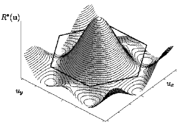
FIG. 2.: Fixed point correlator $\tilde{R^{*}}({\bf u})$. The hexagon represents a Wigner-Seitz cell of the triangular lattice.

FIG. 3.: Variation of $\tilde{\Delta}^{*}=-\tilde{R}_{xx}^{*}({\bf 0})=-\tilde{R}_{yy}^{*}({\bf 0})$ with anisotropy $\delta=1-2\ln\kappa/(\kappa-\kappa^{-1})$.

IV Correlation functions

A Length crossover effects

With the solution of the RG equation at hand, we calculate the disorder and thermal averaged squared relative displacement as a measure of translational order. It is related to the basic correlator of the replica fields

$\displaystyle\langle u_{\alpha}^{a}({\bf q})u_{\beta}^{b}({\bf q}^{\prime})\rangle=T{\mathcal{G}}_{\alpha\beta}^{ab}({\bf q})\,(2\pi)^{d}\delta({\bf q}+{\bf q}^{\prime})$

by

$$B_{\alpha\beta}({\bf r}-{\bf r}^{\prime}) = \overline{\langle[u_{\alpha}({\bf r})-u_{\alpha}({\bf r}^{\prime})][u_{\beta}({\bf r})-u_{\beta}({\bf r}^{\prime})]\rangle}$$ (42)

$$= 2\!\lim_{n\to 0}\int\limits_{{\bf q}}\!\!T{\mathcal{G}}_{\alpha\beta}^{aa}({\bf q})\left(1\!-\!\cos{\bf q}({\bf r}-{\bf r}^{\prime})\right).$$ (43)

If we denote the correlator for a system with a renormalized Hamiltonian ${\mathcal{H}}_{l}^{n}$ by ${\mathcal{G}}_{l}$ and if we allow temperature to flow according to Eq. (27), the scaling relation $T{\mathcal{G}}({\bf q})=T_{l}{\mathcal{G}}_{l}(b{\bf q})b^{2\zeta+d}$ holds for all ${\bf q}$ with $|{\bf q}|\leq\Lambda/b$. To obtain to order $\epsilon$ the exact propagator ${\mathcal{G}}({\bf q})$ for fixed ${\bf q}$, we choose $b=\Lambda/|{\bf q}|$. This allows to employ a harmonic approximation to calculate ${\mathcal{G}}_{l}$ since the coupling of modes with momenta between $|{\bf q}|$ and $\Lambda$ has been taken into account already by the renormalization of ${\mathcal{H}}_{l}^{n}$. Thus we obtain the propagator

$$T{\mathcal{G}}_{\alpha\beta}^{aa}({\bf q}) = \left\{\left({\Lambda\over q}\right)^{d-4}\!\!\!\!\!\!\Delta_{l}\left({\mathcal{G}}_{L}^{2}({\bf q}){\sf P}^{L}_{\alpha\beta}+{\mathcal{G}}_{T}^{2}({\bf q}){\sf P}^{T}_{\alpha\beta}\right)\right.$$ (45)

$$+T\left({\mathcal{G}}_{L}({\bf q}){\sf P}^{L}_{\alpha\beta}+{\mathcal{G}}_{T}({\bf q}){\sf P}^{T}_{\alpha\beta}\right)\Bigg{\}}$$

with $l=\ln{\Lambda/q}$. The term $\sim T$ is the mere thermal propagator. It does not effect roughness in $d>2$ below the melting transition and is thus negligible against the disorder term $\sim\Delta_{l}$ which is more strongly divergent for $|{\bf q}|\to 0$.

Before we discuss the asymptotic displacement correlations in the next Section, we want to exploit the behaviour of $B_{\alpha\beta}({\bf r})$ on intermediate length scales. According to the definition of the roughness exponent $\zeta$ by $B({\bf r})\sim|{\bf r}|^{2\zeta}$ the scaling of the renormalized disorder strength $\Delta_{l}$ determines $\zeta$. It is easily observed from Eq. (45) that necessarily $\ln\Delta_{l}\sim 2\zeta l$ before it reaches its fixed point $\Delta^{*}$ corresponding to $\zeta=0$. The RG flow of $\ln\Delta_{l}$ as a function of $l$ is plotted in Fig. 4.

FIG. 4.: Scaling behaviour of the renormalized disorder strength $\Delta_{l}$ in the three different length scale regimes (solid curve). The random manifold (RM) regime disappears (dashed curve) if the bare $R_{0}({\bf u})$ has non-vanishing Fourier coefficients for the lowest order hexagon only, corresponding to the case $a=\xi$ [see Eq. (22)].

Two qualitative different types of behaviour can be observed, depending on the bare form of the correlator $R_{0}({\bf u})$: (i) If $a=\xi$ only the lowest order harmonics of $R_{0}({\bf u})$ are non-zero and two different scaling regimes with a sharp crossover emerge. The first one is called random force (RF) regime since $\zeta=\zeta_{\rm RF}=\epsilon/2$ as predicted by Larkin’s perturbative approach for a random force model [8], which becomes applicable if $B({\bf r})\lesssim\xi^{2}$. The last scaling regime is the asymptotic (A) one with logarithmic roughness. (ii) If $a>\xi$ also higher order Fourier coefficients are non-zero and a new scaling regime with a non-trivial value of $\zeta$ appears between the RF and A regime. It is called random manifold (RM) regime since here the roughness is expected to be determined by the wandering of lines that do not yet compete with each other for disorder energy minima, i.e., $B({\bf r})\lesssim a^{2}$. But metastability is already important on these length scales leading to a new roughness exponent $\zeta_{\rm RM}$. One of the central results of our analysis is that $\zeta_{\rm RM}$ is nonuniversal. It depends on the ratio $\kappa$ of elastic constants and varies between $0.1737\epsilon$ and $0.1763\epsilon$ as shown in Fig. 5.

FIG. 5.: The roughness exponent $\zeta_{\rm RM}$ is nonuniversal in the RM regime.

The only result for $\zeta_{\rm RM}$, which has been available so far, is based on a Flory type argument for the flux line lattice in that regime [32, 33]. It is given by $\zeta_{RM}=\frac{4-d}{4+N}=\epsilon/6\backsimeq 0.167\epsilon$ ($N$ is the number of components of the displacement field, here $N=2$.) and supposed to be a lower bound, in agreement with our findings. We expect that the range of variation of the nonuniversal $\zeta_{RM}$ is larger in real three dimensions than an epsilon expansion to first order can reveal. This is because in the propagator the effect of variing $c_{11},c_{66}$ is suppressed in an expansion around 4D by the more heavily weighted $c_{44}{\bf q}_{z}^{2}$-term.

Next we calculate the crossover length scales. These are denoted by $L_{\xi}$ and $L_{a}$ for the crossover RF – RM and RM – A, respectively. $L_{\xi}$ can be obtained from Larkin’s perturbative analysis, which yields for the displacement correlations

$$B({\bf r})=\overline{\langle[{\bf u}({\bf x},z)-{\bf u}({\bf 0},0)]^{2}\rangle}\backsimeq\frac{B}{\Phi_{0}}\frac{f^{2}_{pin}n_{imp}\xi^{2}}{\pi c_{44}^{1/2}}$$ (47)

$$\times\left\{c_{11}^{-3/2}({\bf x}^{2}+z_{l}^{2})^{1/2}+c_{66}^{-3/2}({\bf x}^{2}+z_{t}^{2})^{1/2}\right\}.$$

Here we have introduced the rescaled z-coordinates $z_{l}=z\sqrt{c_{11}/c_{44}}$, $z_{t}=z\sqrt{c_{66}/c_{44}}$. The anisotropic crossover or Larkin length scale is determined by the conditions $B({\bf 0},z=L_{\xi}^{z})\simeq\xi^{2}$ and $B(|{\bf x}|=L_{\xi}^{\bf x},0)\simeq\xi^{2}$, thus giving

$$L_{\xi}^{z} \backsimeq \frac{\pi\Phi_{0}}{Bf_{pin}^{2}n_{imp}}\frac{c_{11}c_{44}c_{66}}{c_{11}+c_{66}}$$ (48)

$$L_{\xi}^{\bf x} \backsimeq \frac{\pi\Phi_{0}}{Bf_{pin}^{2}n_{imp}}\frac{c_{44}^{1/2}(c_{11}c_{66})^{3/2}}{c_{11}^{3/2}+c_{66}^{3/2}}.$$ (49)

Based on the condition for the mean displacements of lines at the crossover scales, the second crossover length scales $L_{a}^{z}$, $L_{a}^{\bf x}$ should be related to the Larkin length scales by $L_{a}^{(z,{\bf x})}\simeq(a/\xi)^{1/\zeta_{\rm RM}}L_{\xi}^{(z,{\bf x})}$. To check this relation we have determined the crossover scales numerically from the RG flow of $\Delta_{l}$ for different ratios $a/\xi$. The estimates for $\zeta_{RM}$ thus obtained are consistent with the exact values shown in Fig. 5. Of course, due to the finite extent of the crossover regions, errors are much too large as to take this as a measurement of $\zeta_{RM}$; however, it clearly confirms the physical picture of the crossover lengthscales. Turning to the RG flow of the whole function $R_{l}({\bf u})$, one expects that the appearance of metastability on the Larkin scale should be reflected in a change of the functional form of $R_{l}({\bf u})$, too. Indeed, the existence of a cusp in the RM and A regime can be observed from the sequence of Figures 6, 7, 8 and 9, which show the second radial derivative of $R_{l}({\bf u})$ in the different scaling regimes, see Fig. 4. From this observation we expect that the fourth derivatives $\partial^{4}_{u_{x}}\tilde{R}({\bf 0})=\partial^{4}_{u_{y}}\tilde{R}({\bf 0})\equiv\tilde{R}^{(4)}({\bf 0})$ diverge at the scale given by the Larkin length. The scale $l_{c}=\ln(L_{c}\Lambda)$ at which the cusp appears can be extracted from the RG Eq. (39) as pointed out in Ref. [34] for a different RG equation. Using the relations $\partial^{4}_{x}\tilde{R}({\bf 0})=\partial^{4}_{x}\tilde{R}({\bf 0})=3\partial^{2}_{x}\partial^{2}_{y}\tilde{R}({\bf 0})$ amongst derivatives of the correlator at the lattice sites, we get as equation of flow for the fourth derivative $\tilde{R}^{(4)}({\bf 0})$ at the lattice sites

$$\partial_{l}\tilde{R}^{(4)}({\bf 0})=\epsilon\tilde{R}^{(4)}({\bf 0})+\frac{a^{2}}{3}(10-\delta)\left[\tilde{R}^{(4)}({\bf 0})\right]^{2}.$$ (50)

This equation can be easily integrated and yields in the weak disorder limit for the length scale where first $\tilde{R}^{4}({\bf 0})=\infty$ the result

$$L_{c}=\frac{3}{a^{2}\Lambda(10-\delta)}\frac{1}{\tilde{R}^{(4)}_{0}({\bf 0})}.$$ (51)

Using relation (22), (36) the bare value of $\tilde{R}_{0}^{(4)}$ can be expressed in physical quantities and we get for $\xi\ll a$

$$L_{c}\backsimeq\frac{1}{2}\frac{1}{\rho_{0}f_{pin}^{2}n_{imp}}\frac{c_{44}c_{11}c_{66}}{c_{11}+c_{66}}.$$ (52)

Comparison of this result to the Larkin length of Eq. (48) shows that the correlator $R_{l}({\bf u})$ becomes indeed non-analytic at the crossover to the RM regime.

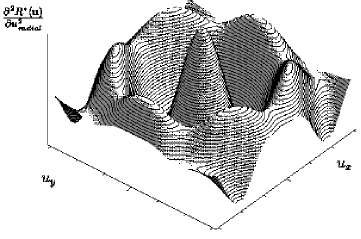
FIG. 6.: Second radial derivative $\partial_{|{\bf u}|}^{2}R({\bf u})$ at the initial position a ($l=0$) shown in Fig. 4.

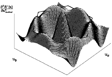
FIG. 7.: Random force regime: $\partial_{|{\bf u}|}^{2}R({\bf u})$ at position b in Fig. 4 obtained by integrating numerically the RG Eq. (39).

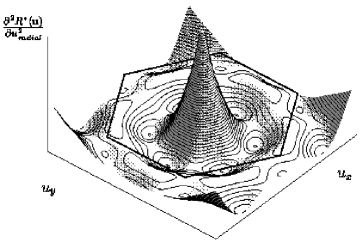
FIG. 8.: Random manifold regime: $\partial_{|{\bf u}|}^{2}R({\bf u})$ at position c in Fig. 4.

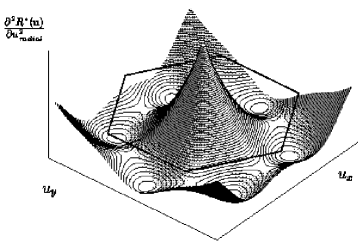
FIG. 9.: Asymptotic fixed point: $\partial_{|{\bf u}|}^{2}R({\bf u})$ at position d in Fig. 4.

B Asymptotic displacement correlations

We now study the correlations in regime A in detail, starting with the displacement correlations. Beyond the second crossover scale $L_{a}$ the larger-$q$ modes governing both the RF and RM regime become unimportant and we may benefit from the fact that $\Delta_{l}\to\Delta^{*}$ in the asymptotic regime. Therefore, the only relevant disorder part of the correlator in Eq. (45) behaves like $T{\mathcal{G}}_{\alpha\beta}^{aa}({\bf q})\sim\Delta^{*}q^{-d}$ leading to logarithmic roughness. It is interesting to note that the amplitude of the displacement correlations $B_{\alpha\beta}({\bf r})$ does not depend on the disorder strength, but is proportional to the fixed point value $\tilde{\Delta}^{*}(\kappa)$, whose dependency on $\kappa$ is shown in Fig. 3. The correlation function $B_{\alpha\beta}({\bf r})$ can now be calculated with explicit consideration of the anisotropic elasticity using Eqs. (42), (45). With the abbreviations $z_{l}=z\sqrt{c_{11}/c_{44}}$, $z_{t}=z\sqrt{c_{66}/c_{44}}$ and $h(t)=t^{-2}\ln(1+t^{2})$ we find in regime A

$$B_{xx}({\bf r}) = \frac{\tilde{\Delta}^{*}(\kappa)a^{2}}{1+\kappa}\left\{\ln\!\left(\frac{{\bf x}^{2}+z_{t}^{2}}{L_{a}^{2}}\right)+\kappa\ln\!\left(\frac{{\bf x}^{2}+z_{l}^{2}}{L_{a}^{2}}\right)\right.$$ (54)

$$+\left.\frac{y^{2}-x^{2}}{{\bf x}^{2}}\left[1-\kappa-h\!\left(\frac{|{\bf x}|}{z_{t}}\!\right)+\kappa\,h\!\left(\frac{|{\bf x}|}{z_{l}}\!\right)\right]\right\},$$

$$B_{yy}({\bf r}) = \frac{\tilde{\Delta}^{*}(\kappa)a^{2}}{1+\kappa}\left\{\ln\!\left(\frac{{\bf x}^{2}+z_{t}^{2}}{L_{a}^{2}}\right)+\kappa\ln\!\left(\frac{{\bf x}^{2}+z_{l}^{2}}{L_{a}^{2}}\right)\right.$$ (56)

$$+\left.\frac{x^{2}-y^{2}}{{\bf x}^{2}}\left[1-\kappa-h\!\left(\frac{|{\bf x}|}{z_{t}}\!\right)+\kappa\,h\!\left(\frac{|{\bf x}|}{z_{l}}\!\right)\right]\right\},$$

$$B_{xy}({\bf r}) = \frac{2\tilde{\Delta}^{*}(\kappa)a^{2}}{1+\kappa}\frac{xy}{{\bf x}^{2}}\left\{\kappa-1-\kappa\,h\!\left(\frac{|{\bf x}|}{z_{l}}\right)+h\!\left(\frac{|{\bf x}|}{z_{t}}\right)\right\}$$ (57)

and thus

$$\begin{split}&\overline{\langle[{\bf u}({\bf r})-{\bf u}({\bf 0})]^{2}\rangle}=B_{xx}({\bf r})+B_{yy}({\bf r})\\ &=\frac{2\,\tilde{\Delta}^{*}(\kappa)a^{2}}{1+\kappa}\left\{\ln\!\left(\frac{{\bf x}^{2}+z_{t}^{2}}{L_{a}^{2}}\right)+\kappa\ln\!\left(\frac{{\bf x}^{2}+z_{l}^{2}}{L_{a}^{2}}\right)\right\}.\end{split}$$ (59)

The details of the Fourier transformation are given in appendix C. There the calculation retaining all unbounded terms for large $|{\bf x}|,z$ is performed in 4D since $\tilde{\Delta}^{*}$ is ${\mathcal{O}}(\epsilon)$. For the reason mentioned in Section II B (b) $B_{yy}({\bf r})$ can be obtained from $B_{xx}({\bf r})$ by $\kappa\rightarrow\kappa^{-1}$. The relative line displacement $B_{\alpha\beta}({\bf r})$ grows only logarithmically due to the restriction of available configurations by adjacent lines. The ‘geometric’ coefficients of the logarithms reflect the elastic anisotropy. The result reminds of the findings for the analogous 2D flux line lattice by Carpentier and Le Doussal, where there is also a nonuniversal prefactor of logarithmic roughness that depends on the elastic details of the system [35].

To compare our results with former results by Giamarchi and Le Doussal (GD) [14, 15] in 3D we consider two limiting cases. First, in the limit $z\to 0$ the relative displacement reduces to

$$B_{xx} = \tilde{\Delta}^{*}(\kappa)a^{2}\left\{\ln\!\left(\frac{{\bf x}^{2}}{L_{a}^{2}}\right)+\frac{x^{2}-y^{2}}{{\bf x}^{2}}\frac{\kappa-1}{\kappa+1}\right\}$$

$$B_{xy} = 2\tilde{\Delta}^{*}(\kappa)a^{2}\frac{xy}{{\bf x}^{2}}\frac{\kappa-1}{\kappa+1}$$

This result is identical in form with the result of GD obtained from a variational ansatz treatment for the triangular lattice. However, this ansatz yields a value for $\tilde{\Delta}^{*}$ which is independent of $\kappa$ and differs from ours by about 15%. The origin of this deviation is the inexact treatment of fluctuations by the variational method. The renormalization group approach of GD is restricted to an idealized scalar field model of a flux line lattice with isotropic elasticity. To determine the influence of the triangular lattice symmetry on $\tilde{\Delta}^{*}$ compared to the scalar model, we consider now the isotropic case $c_{11}=c_{66}$ corresponding to $\kappa=1$. With the rescaled coordinate ${\bf r}^{\prime}=({\bf x},\sqrt{c_{11}/c_{44}}z)$ we obtain

$$B_{xx}=B_{yy}=2\tilde{\Delta}^{*}(1)a^{2}\ln(|{\bf r}^{\prime}|/L_{a}),\quad B_{xy}=0$$

with $\tilde{\Delta}^{*}(1)=0.0217\epsilon$. This has to be compared to the result $\tilde{\Delta}^{*}(1)=\epsilon/36\simeq 0.028\epsilon$ for the scalar model.

C Order parameters

Now we study the translational order parameter $\Psi_{\bf G}({\bf r})\equiv e^{i{\bf G}{\bf u}({\bf r})}$ to measure the remaining translational order in the impure system. The pair correlation function is

$$C_{{\bf G}}({\bf r})=\overline{\langle\Psi_{\bf G}({\bf r})\Psi^{*}_{\bf G}({\bf 0})\rangle}=\overline{\langle e^{i{\bf G}({\bf u}({\bf r})-{\bf u}({\bf 0}))}\rangle}.$$ (60)

It is a preferred measure, as its scaling behaviour determines the intensity of the reflection pattern obtained in neutron scattering, see below. $C_{\bf G}({\bf r})$ is often referred to as translational order correlation or simply ‘translational order’. Being exact to order $\epsilon$, the average can be raised to the exponent as if ${\bf u}({\bf r})$ was Gaussian distributed [36]. We thus can obtain from Eq. (54) the result for the asymptotic scaling regime,

$$C_{\bf G}({\bf r}) \propto g_{\bf G}L_{a}^{\eta_{\bf G}(\kappa)}({\bf x}^{2}+z_{t}^{2})^{-\frac{\eta_{\bf G}(\kappa)}{2(1+\kappa)}}$$ (62)

$$\times({\bf x}^{2}+z_{l}^{2})^{-\frac{\eta_{\bf G}(\kappa)}{2(1+1/\kappa)}}$$

with exponent

$$\eta_{\bf G}(\kappa)=\tilde{\Delta}^{*}(\kappa)(aG)^{2}$$ (63)

and the geometrical factor

$$g_{\bf G} = \exp\left[\frac{\tilde{\Delta}^{*}(\kappa)(aG)^{2}}{1+\kappa}\left((\hat{\bf x}\hat{\bf G})^{2}-\frac{1}{2}\right)\!\,\right.$$ (65)

$$\,\left.\times\left\{\!\left(\!1-h\!\left(\frac{|{\bf x}|}{z_{t}}\right)\!\!\right)-\kappa\left(\!1-h\!\left(\frac{|{\bf x}|}{z_{l}}\right)\!\!\right)\!\right\}\right].$$

Our main result on the translational order of the flux line lattice consists in the decay of order with a nonuniversal exponent $\eta_{\bf G}(\kappa)$. Its dependency on $\kappa$ is obtained from Eq. (63) and is shown in Fig. 10 for one of the smallest reciprocal lattice vectors ${\bf G}={\bf G}_{0}$ with $|{\bf G}_{0}|=4\pi/(a\sqrt{3})$. The full decay exponent in Eq. (62) is modified by additional $\kappa$-dependent factors due to the anisotropic elasticity leading to different decay of contributions from transversal and longitudinal modes. The nonuniversal behaviour is at variance with the variational ansatz results and conjectures in Refs. [14, 15].

Let us consider the two limiting cases from above: For $z\rightarrow 0$ the result simplifies to

$$C_{\bf G}({\bf x}) \propto (|{\bf x}|/L_{a})^{-\eta_{\bf G}(\kappa)}$$ (66)

$$\times \exp\left\{\tilde{\Delta}^{*}(\kappa)(aG)^{2}\frac{1-\kappa}{1+\kappa}\left((\hat{\bf x}\hat{\bf G})^{2}-\frac{1}{2}\right)\right\},$$ (67)

which again coincides modulo the difference in the coefficent with the result found by GD for this limit. For $\kappa=1$, the translational order decay is isotropic according to

$\displaystyle C_{\bf G}({\bf r}^{\prime})\propto L_{a}^{\eta_{\bf G}(1)}{|{\bf r}^{\prime}|}^{-\eta_{\bf G}(1)}$

with the rescaled coordinate ${\bf r}^{\prime}$ defined above. This isotropic limit can be used to demonstrate clearly that the triangular flux line lattice considered here and the scalar model do not belong to the same universality class. Whereas we obtain $\eta_{\bf G}(1)=1.14\epsilon$ for the triangular lattice, the result in the RG approach for the scalar model – which corresponds to a square lattice – is $\eta_{\bf G}(1)=\pi^{2}/9\epsilon=1.10\epsilon$.

FIG. 10.: Dependency of the exponent $\eta_{{\bf G}_{0}}$ on the ratio $\kappa=c_{66}/c_{11}$ of elastic constants.

Another order parameter of interest is the positional glass correlation function suggested by spin glass theory [37]

$$S_{PG}({\bf G},{\bf r})=\overline{\left|\langle\Psi_{\bf G}({\bf r})\Psi^{*}_{\bf G}({\bf 0})\rangle\right|^{2}}.$$ (68)

It measures the thermal fluctuations of the flux lines around their disordered ground state. We calculate $S_{PG}({\bf G},{\bf r})$ within our framework from the hamiltonian renormalized up to scale $|{\bf r}|=\Lambda^{-1}e^{l}$. First order perturbation theory in the pinning energy gives the corrections to the mere thermal result to first order in $\epsilon$. We get

$$S_{PG}({\bf G},{\bf r})\backsimeq S_{PG}^{0}({\bf G},{\bf r})\left\{1+\epsilon\sum_{m\geq 1}c_{m}\left({T\over r^{2}}\right)^{2m}\right\},$$ (69)

where $S_{PG}^{0}({\bf G},{\bf r})$ denotes the correlation function for the pure system with thermal fluctuations only and $c_{m}$ are numerical coefficients. It is finite for $r\rightarrow\infty$ and reduced with respect to unity merely by the standard Debye-Waller factor. As the order $\epsilon$ corrections decay they can surely not compensate the leading constant term and make up for a more than powerlaw decay of the whole correlation function. This provides signature of a positional glass to order $\epsilon$.

Widely discussed, however not completely resolved is the question, if there exists a phase coherent vortex glass state in impure type-II superconductors. A finite value of the correlation function

$$C_{V\!G}({\bf r})=\overline{\left|\langle\Psi({\bf r})\Psi^{*}({\bf 0})\rangle\right|^{2}}$$ (70)

for large $|{\bf r}|$ is proposed to identify such a phase coherent vortex glass [38, 39]. Here $\Psi({\bf r})$ is the Ginzburg-Landau complex order parameter. It can be decomposed in amplitude and phasefactor, $\Psi=|\Psi|e^{i[\phi_{0}+\delta\phi]}$, with groundstate phase $\phi_{0}$ and phase fluctuations $\delta\phi$. In the London limit the amplitude is constant outside the vortices and $C_{V\!G}$ becomes

$$C_{V\!G}({\bf r})=|\Psi|^{2}\overline{|\langle e^{i[\delta\phi({\bf r})-\delta\phi({\bf 0})]}\rangle|^{2}}.$$ (71)

Since the phase fluctuations are topologically constrained by the vortex positions, the distortions of the vortex lattice can destroy phase coherence. More concrete, phase fluctuations and vortex displacements are related by [40]

$$\nabla^{2}\delta\phi({\bf r})={{2\pi}\over a}\left(\nabla_{\perp}\times{\bf u}({\bf r})\right).$$ (72)

This relation allows for the calculation of $C_{V\!G}({\bf r})$ in the framework of the elastic description of the flux line lattice. We use perturbation theory for ${\mathcal{H}}_{dis}$ with fluctuations on scales below $|{\bf r}|$ having renormalized this perturbation. Then corrections to the mere thermal average $\langle\ldots\rangle_{0}$ are given to first order in $\epsilon$ by

$$\begin{split}&C_{V\!G}({\bf r})=e^{-\langle[\delta\phi({\bf r})-\delta\phi({\bf 0})]^{2}\rangle_{0}}\times\Big{\{}1\\ &+{1\over T^{2}}\sum_{\bf G}\hat{R}^{*}_{\bf G}\int_{\bar{\bf r}}\left[\cosh(2F({\bf r},\bar{\bf r}))-4\cosh(F({\bf r},\bar{\bf r}))\right]\Big{\}}.\end{split}$$ (73)

Here $\hat{R}_{\bf G}^{*}=R_{\bf G}^{*}\exp(-G_{\alpha}G_{\beta}\langle u_{\alpha}({\bf 0})u_{\beta}({\bf 0})\rangle_{0})\sim\epsilon$ are the reduced Fourier coefficients of the random energy correlator of Eq. (20) and $F({\bf r},\bar{\bf r})=\Gamma({\bf r}-\bar{\bf r})-\Gamma(-\bar{\bf r})$ with $\Gamma({\bf r})=\langle{\bf G}{\bf u}({\bf r})\delta\phi({\bf 0})\rangle_{0}$. The exponential factor of $\hat{R}_{\bf G}^{*}$ is finite in $d>2$. For the disorder induced correction in Eq. (LABEL:CVG) we focus on the isotropic limit with $c_{44}=c_{66}$ and get

$$\Gamma({\bf r})={T\over{4\pi a^{2}c_{44}}}\frac{G_{y}x-G_{x}y}{r^{2}}\left(1-{2\over{\Lambda r}}J_{1}(\Lambda r)\right),$$ (74)

where $J_{1}(x)$ is the Besselfunction of first kind. Upon expansion of the $\cosh$-terms, a careful investigation of the behaviour for large $|{\bf r}|$ of the remaining integrals gives to order $\epsilon$

$$\begin{split}&C_{V\!G}({\bf r})\simeq e^{-\langle[\delta\phi({\bf r})-\delta\phi({\bf 0})]^{2}\rangle_{0}}\\ &\times\left\{1+\epsilon\left[d_{1}T^{2}\ln(r\Lambda)+d_{2}+\sum_{m\geq 0}c_{m}T^{2}\left({T\over r}\right)^{2m}\right]\right\}.\end{split}$$ (75)

The $d_{i},c_{i}$ are again numerical coefficients, yet different from the ones in Eq. (69). The exponential factor of Eq. (LABEL:CVG) is determined by mere thermal fluctuations, which read

$$\begin{split}\langle[\delta\phi({\bf r})&-\delta\phi({\bf 0})]^{2}\rangle_{0}\\ &={{8\pi^{2}}\over{a^{4}}}\,T\int_{\bf q}{q_{\perp}^{2}\over q^{4}}{\mathcal{G}}^{T}({\bf q})[1-\cos({\bf q}{\bf r})]\sim{1\over\epsilon}|{\bf r}|^{\epsilon}.\end{split}$$ (76)

Corrections to order $\epsilon$ can thus not compete against the exponential decay of $C_{V\!G}({\bf r})$ originating from strong thermal fluctuations. Thus we conclude that to order $\epsilon$ there is no phase coherent vortex glass. Whether this result is valid to higher orders in $\epsilon$ and thus in 3D remains however unclear within the present analysis. Dorsey et al. [41] indeed found a vortex glass transition in $6-\epsilon$ dimensions starting from a Ginzburg-Landau Hamiltonian. If this transition exists down to three dimensions is not clear.

D Experimental implications

There exists a considerable number of recent experimental studies of the structure of flux line lattices in high temperature superconductors. Neutron diffraction studies provide strong evidence for the proposed Bragg glass with quasi-longrange order [5, 6, 42]. More recently, magnetic decoration studies on BSCCO showed huge dislocation free regions containing up to $10^{5}$ flux lines [22]. The last result strongly supports our elastic description, which neglects dislocations.

Comparison with neutron diffraction experiments shows the preferred role of the translational order correlation $C_{{\bf G}}({\bf r})$. The diverging dependency of the cross section in a neutron scattering experiment is given by

$$\sigma({\bf k})\propto\overline{\langle\rho_{\bf k}\>\rho_{-{\bf k}}\rangle}\propto\tilde{S}({\bf k}),$$ (77)

where ${\bf k}=({\bf k}_{\perp},k_{z})$ is the difference between in- and outgoing wavevectors and $\rho_{\bf k}$ the Fourier transform of the flux line density in Eq. (9). The structure factor $\tilde{S}({\bf k})$ is the Fourier transform of the density-density correlation. Close to a reciprocal lattice vector,

$$k_{z}\equiv q_{z},\quad{\bf k}_{\perp}\equiv{\bf G}+{\bf q}_{\perp},\quad{\bf q}_{\perp}\ll G,$$

the structure factor becomes

$$\tilde{S}({\bf G}+{\bf q}_{\perp},q_{z}) = \int_{z}\sum_{\bf X}e^{iq_{z}z+i{\bf q}_{\perp}{\bf X}}\overline{\langle e^{i({\bf G}+{\bf q}_{\perp})({\bf u}({\bf X},z)-{\bf u}({\bf 0},0))}\rangle}$$ (78)

$$\simeq \int d^{3}re^{iq_{z}z+i{\bf q}_{\perp}{\bf x}}C_{{\bf G}}({\bf r}).$$ (79)

The scattered intensity is thus described by the Fourier transform of the translational order correlation $C_{{\bf G}}({\bf r})$ defined in Eq. (60). The Fourier transformation can be done numerically for general $\kappa$ but one can see easily that the power law decay of $C_{{\bf G}}({\bf r})$ is slow enough to effect powerlaw divergence of $\tilde{S}({\bf G}+{\bf q}_{\perp},q_{z})$ for small ${\bf q}_{\perp}$. For the limiting cases $c_{11}=c_{66},\kappa=1$ and $c_{11}\gg c_{66},\kappa\backsimeq 0$, of which the latter is realized physically close to $H_{c_{2}}$, the structure factor reads

$$\tilde{S}({\bf G}+{\bf q}_{\perp},q_{z})\propto\left({\bf q}_{\perp}^{2}+{{c_{44}}\over{c_{66}}}q_{z}^{2}\right)^{(-3+\eta_{\bf G}(\kappa))/2}.$$ (80)

As a consequence of the quasi-long-range order in the asymptotic regime beyond the scale $L_{a}$, the structure factor diverges for small (${\bf q}_{\perp},q_{z}$) leading to Bragg peaks. Giamarchi and Le Doussal thereafter named the weakly disordered flux line lattice a Bragg-glass.

In experiments, Bragg peaks and their disappearence for higher magnetic fields due to a melting of the flux line lattice have in fact been observed in BSCCO [5, 6]. However, quantitative details of the divergence cannot be resolved putting our prediction of nonuniversality of $\eta_{\bf G}$ beyond the precision of today’s experimental diffraction techniques. But there exist recent experimental results which are based on a more microscopic way to determine the structure of flux line lattices. Kim et al. use a scanning electron microscope to obtain a spatial map of the flux line displacements itself over a region containing about $5\cdot 10^{5}$ lines [22]. Due to the small coherence length of $\approx 20\AA$ in BSCCO we have $\xi\ll a$ so that only the RM and A regime can be observed in principle. Experimental results for the mean squared relative displacement of lines are available in the RM regime, whereas the asymptotic regime is beyond the experimental limit. Kim et al. measure in this regime a roughness exponent of $\zeta_{RM}=0.22$. This result is in reasonable agreement with our first order $\epsilon$ expansion result of $\zeta_{RM}\approx 0.18$ in 3D.

V Discussion and conclusion

For the first time, the three dimensional Abrikosov lattice in the presence of point disorder has been treated within a renormalization group procedure including all of the elastic modes. Triangular symmetry complicates the calculation of large scale 3D correlation functions in their anisotropic dependency on position arguments. These technical difficulties could be overcome and we can write correlations in their full anisotropy. More important however, translational quasi-long-range order in impure type-II superconductors is described by a – contrary to previous claims – nonuniversal power-like decay of the order parameter correlations. In particular, the decay-exponent $\eta_{\bf G}$ depends (if weakly) on the ratio $\kappa=c_{66}/{c}_{11}$ of the elastic constants.

In isotropic superconductors at low temperatures, where flux lines interact via central forces, one has $0\leq\kappa\leq 1/3$. $\kappa\sim 1/3$ for $\lambda\leq a$, i.e. for fields close to $H_{c_{1}}$, and $\kappa\rightarrow 0$ for $H\rightarrow H_{c_{2}}$. For most of the field region $\kappa\approx\phi_{0}/16\pi\lambda^{2}B$,. Thus, an increase of the external field from $H_{c_{1}}$ to $H_{c_{2}}$ should result in an increase of $\eta_{{\bf G}}$ and a decrease of $\zeta_{RM}$. Numerically, the effect is small, since $\eta_{{\bf G}_{0}}$ ranges from $1.145$ to $1.159$ and $\zeta_{rm}$ from $0.1745$ to $0.1763$ in this $\kappa$-range. Thus it will probably be hard to detect this effect. However, we are likely to have suppressed some of the nonuniversality in our calculation when we extended the $z$-direction to 2 dimensions. In the propagator the effect of variations in $c_{11}$ and $c_{66}$ is thus reduced by the more heavily weighted $c_{44}{\bf q}_{z}^{2}$-term. The behaviour of 2D disordered triangular lattices supports this point of view. Here, Carpentier and Le Doussal obtain nonuniversal large scale behaviour that is much more pronounced than in our higher dimensional case [35]. The small quantity of the calculated effect should thus not mislead to underestimate its qualitative relevance.

Different from usual RG approaches we observed the full flow of renormalization of the the interaction. We thus gained in addition to the fixed point dominated large scale behaviour information on the intermediate length scales. We find a crossover of the structural correlation functions from a Larkin-regime, where perturbation theory applies, to the random manifold regime and eventually to the asymptotic Bragg glass regime. Out of one Hamiltonian this confirms most clearly the physical picture that had originated over many years from different approximation strategies to this prominent physical system. For the random manifold regime, where fluxlines explore many minima in the energy landscape but do not yet compete against each other, we could extract the roughness exponent numerically from the flow. This is valuable in itself as it can be compared only to an estimated exponent from scaling arguments. Moreover it also shows dependency on elastic constants, i.e., is nonuniversal.
Dislocations are excluded in our description. Whereas the stability of the Bragg-glass phase against these topological defects had not always been commonly agreed upon, today the position of the Bragg-glass in the phase diagram is well established. In the $H-T$ plane at not too large fields, weak disorder – the definition of which can be cast into a Lindemann criterion – has the Abrikosov phase of the pure phase diagram become the Bragg-glass. It is bounded by a first order transition melting line with negative slope, just like the Abrikosov phase in the pure system. This line ends at a critical point. For larger fields and small temperatures the Bragg-glass is bounded by the proliferation of vortices that destroy quasi-long-range order [17, 16, 19, 18, 21, 20]. The exact nature of the large field state – it may be called a dislocated vortex glass – is not clearly understood, nor is the transition (or mere crossing) into it from the Bragg-glass. Berker set up a criterion for the shift of a first order transition to a second order one by disorder [43]. For a sharp domain boundary at the coexistence point he finds a pure first order transition to be stable against disorder fluctuations above 2D. This is applicable to the melting line where a jump in the FL density, which plays the role of a scalar order parameter, assures the sharp boundary and a first order transition is observed both in pure and impure samples [42].

We would like to thank very much H. E. Brandt, M. Kardar and S. Scheidl for valuable discussions. Financial support was obtained through Deutsche Forschungsgemeinschaft under grant No. EM70/1-3 (T.E.).

A Replica pinning energy

We want to write the replica pinning energy in compact form starting from the pinning energy expression (17). The ${\bf G}\neq{\bf 0}$-terms are the relevant ones, as we have argued.

$${\mathcal{H}}_{dis}^{n}[\{{\bf u}^{a}\}]=$$ (A1)

$$= -{1\over 2T}\overline{\Big{[}\rho_{0}\int_{\bf r}V_{dis}({\bf r})\sum_{{\bf G}\neq{\bf 0}}\sum_{a=1}^{n}e^{i{\bf G}[{\bf x}-{\bf u}^{a}({\bf r})]}\Big{]}^{2}}$$ (A2)

$$= -{1\over 2T}\rho_{0}^{2}\sum_{a,b}\int_{{\bf r}{\bf r}^{\prime}}\Delta_{\xi}({\bf x}-{\bf x}^{\prime})\delta(z-z^{\prime})$$ (A4)

$$\hskip 28.45274pt\times\sum_{{\bf G}{\bf G}^{\prime}}e^{i{\bf G}[{\bf x}-{\bf u}^{a}({\bf r})]+i{\bf G}^{\prime}[{\bf x}^{\prime}-{\bf u}^{b}({\bf r}^{\prime})]}.$$

We focus on the ${\bf x},{\bf x}^{\prime}$-dependency and suppress the $z$-index of the displacement fields for shorter notation.

$$\sum_{{\bf G}{\bf G}^{\prime}}\int_{{\bf x}{\bf x}^{\prime}}\!\!\!\Delta_{\xi}({\bf x}-{\bf x}^{\prime})e^{i{\bf G}[{\bf x}-{\bf u}^{a}({\bf x})]+i{\bf G}^{\prime}[{\bf x}^{\prime}-{\bf u}^{b}({\bf x}^{\prime})]}=$$ (A5)

$$= \sum_{{\bf G}}\int_{{\bf x}}e^{-i{\bf G}[{\bf u}^{a}({\bf x})-{\bf u}^{b}({\bf x})]}\sum_{{\bf G}^{\prime}}e^{i[{\bf G}+{\bf G}^{\prime}][{\bf x}-{\bf u}^{b}({\bf x})]}$$ (A7)

$$\times\int_{\bar{\bf x}}\Delta_{\xi}(\bar{\bf x})e^{i{\bf G}^{\prime}[\bar{\bf x}-({\bf u}^{b}({\bf x}+\bar{\bf x})-{\bf u}^{b}({\bf x}))]}$$

$$\backsimeq \sum_{{\bf G}}\int_{{\bf x}}e^{-i{\bf G}[{\bf u}^{a}({\bf x})-{\bf u}^{b}({\bf x})]}$$ (A9)

$$\times\Big{(}\tilde{\Delta}({\bf G})+\sum_{{\bf G}^{\prime}\neq-{\bf G}}e^{i[{\bf G}+{\bf G}^{\prime}][{\bf x}-{\bf u}^{b}({\bf x})]}\tilde{\Delta}({\bf G}^{\prime})\Big{)}$$

$$\backsimeq \int_{{\bf x}}\sum_{{\bf G}}\tilde{\Delta}({\bf G})e^{-i{\bf G}[{\bf u}^{a}({\bf x})-{\bf u}^{b}({\bf x})]}.$$ (A10)

$\tilde{\Delta}({\bf k})$ is the Fourier transform of $\Delta_{\xi}({\bf x})$, it is nonzero over a region of size $\xi^{-1}$. For the first approximation the slow variation of $[{\bf u}^{b}({\bf x}+\bar{\bf x})-{\bf u}^{b}({\bf x})]$ with $\bar{\bf x}$ is used. In the region $|\bar{\bf x}|\leq\xi$, which is the one contributing to the integral, its variation is negligable versus $\bar{\bf x}$. In the last step, rapidly oscillating terms are neglected versus the constant $\tilde{\Delta}({\bf G})$ as they are both multiplied by the slowly oscillating $e^{-i{\bf G}[{\bf u}^{a}({\bf x})-{\bf u}^{b}({\bf x})]}$ and integrated over.
This gives the replica pinning energy as stated in equation (19)

$${\mathcal{H}}_{dis}^{n}[\{{\bf u}^{a}\}] = -{1\over 2T}\sum_{a,b}\int_{{\bf r}}\rho_{0}^{2}\sum_{{\bf G}\neq{\bf 0}}\tilde{\Delta}({\bf G})e^{-i{\bf G}[{\bf u}^{a}({\bf r})-{\bf u}^{b}({\bf r})]}$$ (A11)

$$\equiv -{1\over 2T}\sum_{a,b}\int_{{\bf r}}R({\bf u}^{a}({\bf r})-{\bf u}^{b}({\bf r})).$$ (A12)

In this version of the replica pinning energy, the effective disorder correlator $R({\bf u})$ is invariant under the full symmetry of the triangular lattice. This is because pinning energy depends only on the positions ${\bf X}+{\bf u}_{\bf X}(z)$ of the vortices. Redistributing the fluxlines to reference positions, i.e., relabelling, may thus not show. ${\mathcal{H}}_{dis}$ in Eq. (7) is consistently invariant under ${\bf u}_{\bf X}(z)\rightarrow{\bf u}_{{\bf X}+{\bf Y}}(z)+{\bf Y}$ with ${\bf Y}$ a constant lattice vector. This reads $\tilde{{\bf u}}(\tilde{{\bf x}})\rightarrow\tilde{{\bf u}}(\tilde{{\bf x}})+{\bf Y}$ after substitution (13) and explains the discrete translational invariance of the Fourier sum $R({\bf u})$.
The point group symmetries also arise from the invariance of disorder energy under a change of the ‘original’ positions of the fluxlines in the pure system. Let us again resume the distinct notation for the field before (${\bf u}({\bf x})$) and after ($\tilde{{\bf u}}(\tilde{{\bf x}})$) substitution (13).

$$\tilde{{\bf u}}(\tilde{{\bf x}})\rightarrow{\sf D}_{60^{\circ}}\tilde{{\bf u}}(\tilde{{\bf x}})$$ (A13)

is not an exact symmetry of the pinning energy, it is rather the transformation

$$\tilde{{\bf u}}(\tilde{{\bf x}})\rightarrow{\sf D}_{60^{\circ}}\tilde{{\bf u}}(\tilde{{\bf x}})+(1-{\sf D}_{60^{\circ}})\tilde{{\bf x}},$$ (A14)

i.e.,

$$\tilde{{\bf x}}-\tilde{{\bf u}}(\tilde{{\bf x}})\rightarrow{\sf D}_{60^{\circ}}(\tilde{{\bf x}}-\tilde{{\bf u}}(\tilde{{\bf x}}))$$ (A15)

that leaves ${\mathcal{H}}_{dis}$ unchanged, as can be seen in (11) (the rotation is absorbed in the reciprocal lattice, that is mapped onto itself as ${\sf D}_{60^{\circ}}$ is a lattice symmetry). For the local term ${\bf G}=-{\bf G}^{\prime}$ that we keep for the final compact form of the pinning energy, symmetry (A14) becomes symmetry (A13). It reads for $\{{\bf x},{\bf u}({\bf x})\}$

$${\bf u}({\bf x})\rightarrow{\bf u}({\sf D}_{60^{\circ}}^{-1}{\bf x})+({\sf D}_{60^{\circ}}^{-1}-1){\bf x}.$$ (A16)

The disorder energy in Eq. (7) is transformed as

$$\sum_{{\bf X}}\int\!{\mbox{d}}z^{d-2}\!\>V_{dis}\left({\bf X}+{\bf u}\left({\bf X}\right),z\right)\rightarrow$$

$$\sum_{{\bf X}}\int\!{\mbox{d}}z^{d-2}\!\>V_{dis}\left({\sf D}_{60^{\circ}}^{-1}{\bf X}+{\bf u}\left({\sf D}_{60^{\circ}}^{-1}{\bf X}\right),z\right)$$

and is invariant as the lattice can be relabelled ${\bf X}\rightarrow{\sf D}_{60^{\circ}}{\bf X}$. Our starting Hamiltonian (19) for the RG is written in the quantities with the tilde. Correlations calculated above are thus also expressed in $\{\tilde{{\bf x}},\tilde{{\bf u}}\}$. For any roughness with exponent smaller than one however, correlations of $\tilde{{\bf u}}$ coincide with the ones of ${\bf u}$. This justifies our dropping of the tilde in most of the treatment above.

B Integrals for the equation of flow

In this appendix the coefficients ${\sf M}$ of equation (30) are calculated.

$${\sf M}^{\alpha\beta,\gamma\delta} = {\mbox{d}}l^{-1}\int_{\bf q}^{>}{\mathcal{G}}_{\alpha\beta}({\bf q}){\mathcal{G}}_{\gamma\delta}(-{\bf q})$$

with

$${\mathcal{G}}_{\alpha\beta}({\bf q}){\mathcal{G}}_{\gamma\delta}(-{\bf q}) = {\sf P}_{\alpha\beta}^{L}{\sf P}_{\gamma\delta}^{L}\left({\mathcal{G}}^{L}\right)^{2}+{\sf P}_{\alpha\beta}^{T}{\sf P}_{\gamma\delta}^{T}\left({\mathcal{G}}^{T}\right)^{2}$$

$$+\left({\sf P}_{\alpha\beta}^{L}{\sf P}_{\gamma\delta}^{T}+{\sf P}_{\alpha\beta}^{T}{\sf P}_{\gamma\delta}^{L}\right).{\mathcal{G}}^{L}{\mathcal{G}}^{T}.$$

The projectors ${\sf P}^{L,T}$ are given after equation (3). Take $(\alpha\beta),\>(\gamma\delta)$ as column- and row-indices of a $4\times 4$ array. The indices shall run through $(xx,xy,yx,yy)$. Then

$$\int_{\bf q}^{>}{\sf P}_{\alpha\beta}^{L}{\sf P}_{\gamma\delta}^{L}\left({\mathcal{G}}^{L}\right)^{2} = {1\over 8}\left(\begin{array}[]{cccc}3&0&0&1\\ 0&1&1&0\\ 0&1&1&0\\ 1&0&0&3\end{array}\right)\int_{\bf q}^{>}{\mathcal{G}}_{L}^{2}.$$

Here the relations

$$\int_{\bf q}^{>}{\mathcal{G}}_{L}^{2}{q_{y}^{4}\over q_{\perp}^{4}}=3\int_{\bf q}^{>}{\mathcal{G}}_{L}^{2}{q_{x}^{2}q_{y}^{2}\over q_{\perp}^{4}},$$

$$2 \int_{\bf q}^{>}\left[{\mathcal{G}}_{L}^{2}{q_{y}^{4}\over q_{\perp}^{4}}+{\mathcal{G}}_{L}^{2}{q_{x}^{2}q_{y}^{2}\over q_{\perp}^{4}}\right]=$$

$$= \int_{\bf q}^{>}{\mathcal{G}}_{L}^{2}{1\over{q_{\perp}^{4}}}(q_{y}^{4}+2q_{y}^{2}q_{x}^{2}+q_{x}^{4})=\int_{\bf q}^{>}{\mathcal{G}}_{L}^{2}$$

have been used. Similarily, one obtains

$$\int_{\bf q}^{>}{\sf P}_{\alpha\beta}^{T}{\sf P}_{\gamma\delta}^{T}\left({\mathcal{G}}^{T}\right)^{2} = {1\over 8}\left(\begin{array}[]{cccc}3&0&0&1\\ 0&1&1&0\\ 0&1&1&0\\ 1&0&0&3\end{array}\right)\int_{\bf q}^{>}{\mathcal{G}}_{T}^{2}$$

and

$$\int_{\bf q}^{>}{\sf P}_{\alpha\beta}^{T}{\sf P}_{\gamma\delta}^{L}{\mathcal{G}}^{L}{\mathcal{G}}^{T} = {1\over 8}\left(\begin{array}[]{cccc}2&0&0&6\\ 0&-2&-2&0\\ 0&-2&-2&0\\ 6&0&0&2\end{array}\right)\int_{\bf q}^{>}{\mathcal{G}}_{T}{\mathcal{G}}_{L}.$$

This gives ${\sf M}^{\alpha\beta,\gamma\delta}$ as stated in (32)

$\displaystyle{\sf M}={1\over 8}\left(\begin{array}[]{cccc}3I_{1}+2I_{2}&0&0&I_{1}+6I_{2}\\ 0&I_{1}-2I_{2}&I_{1}-2I_{2}&0\\ 0&I_{1}-2I_{2}&I_{1}-2I_{2}&0\\ I_{1}+6I_{2}&0&0&3I_{1}+2I_{2}\end{array}\right)$

with

$\displaystyle\begin{array}[]{cc}I_{1}\equiv dl^{-1}\int_{\bf q}^{>}\left({\mathcal{G}}^{2}_{T}+{\mathcal{G}}^{2}_{L}\right)&\quad I_{2}\equiv dl^{-1}\int_{\bf q}^{>}{\mathcal{G}}_{T}{\mathcal{G}}_{L}\end{array}.$

These integrals are evaluated exactly in $d=4$ to

$\displaystyle I_{1}={1\over{8\pi^{2}}}{{1+\kappa}\over{c_{44}c_{66}}}\quad I_{2}=\frac{1}{8\pi^{2}c_{44}c_{11}}\frac{\ln\kappa}{\kappa-1}$

with $\kappa={{c_{66}}/{c_{11}}}$.

C Fourier transform of the anisotropic propagator

In this appendix the displacement correlation functions shall be calculated from the propagator $\overline{\langle u_{\alpha}({\bf q})u_{\beta}({\bf q}^{\prime})\rangle}$ in Eq. (45). The Fourier transformation reads

$\displaystyle B_{\alpha\beta}({\bf r})=2\int_{{\bf q}{\bf q}^{\prime}}^{L_{a}^{-1}}\!\!\overline{\langle u_{\alpha}({\bf q})u_{\beta}({\bf q}^{\prime})\rangle}(1-\cos{\bf q}{\bf r}).$

We integrate in $d=4$ with the $z$-direction extended to a 2D subspace. The $xx$-displacement correlations then are

$$B_{xx}({\bf x},{\bf z})=$$

$$= C\int\!{\mbox{d}}^{4}\!q\>\left(1-\cos({\bf q}_{z}{\bf z}+{\bf q}_{\perp}{\bf x})\right)$$

$$\times\left[\frac{q_{x}^{2}}{q_{\perp}^{2}}{\mathcal{G}}_{L}^{2}+\frac{q_{y}^{2}}{q_{\perp}^{2}}{\mathcal{G}}_{T}^{2}\right]$$

$$= C\int\!{\mbox{d}}^{4}\!q\>\left\{1-\cos({\bf q}_{z}{\bf z})\cos({\bf q}_{\perp}{\bf x})+\sin({\bf q}_{z}{\bf z})\sin({\bf q}_{\perp}{\bf x})\right\}$$

$$\times\left[\frac{q_{x}^{2}}{q_{\perp}^{2}}{\mathcal{G}}_{L}^{2}+\frac{q_{y}^{2}}{q_{\perp}^{2}}{\mathcal{G}}_{T}^{2}\right]$$

$$= C\int\!{\mbox{d}}^{2}\!q_{z}\left\{\int\!{\mbox{d}}q_{\perp}q_{\perp}{\mathcal{G}}_{L}^{2}\int_{0}^{2\pi}\!{\mbox{d}}\phi\left[1-\cos({\bf q}_{z}{\bf z})\right.\right.$$

$$\times\cos(q_{\perp}x\cos\phi+q_{\perp}y\sin\phi)$$

$$+\left.\sin({\bf q}_{z}{\bf z})\sin(q_{\perp}x\cos\phi+q_{\perp}y\sin\phi)\right]\cos^{2}\phi$$

$$\left.+{\mathcal{G}}_{T}\mbox{-analogue}\right\}$$

with $C=2\Delta^{*}(2\pi)^{-4}$. The $\sin({\bf q}_{z}{\bf z})$-term does not contribute as it is antisymmetric in ${\bf q}_{z}$. So we have

$$B_{xx}({\bf x},{\bf z})=$$

$$= C\pi\int\!{\mbox{d}}^{2}q_{z}\int\!{\mbox{d}}q_{\perp}q_{\perp}\Big{\{}{\mathcal{G}}_{L}^{2}\Big{[}1-\cos({\bf q}_{z}{\bf z})$$

$$\times\Big{(}J_{0}(q_{\perp}|{\bf x}|)+\frac{y^{2}-x^{2}}{{\bf x}^{2}}J_{2}(q_{\perp}|{\bf x}|)\Big{)}\Big{]}$$

$$+{\mathcal{G}}_{T}^{2}\Big{[}1-\cos({\bf q}_{z}{\bf z})$$

$$\times\Big{(}J_{0}(q_{\perp}|{\bf x}|)+\frac{x^{2}-y^{2}}{{\bf x}^{2}}J_{2}(q_{\perp}|{\bf x}|)\Big{)}\Big{]}\Big{\}}$$

with $J_{n}$ the Bessel function of the $n$-th kind. We used

$$\int_{0}^{2\pi}\!{\mbox{d}}\phi\cos(q_{\perp}x\cos\phi+q_{\perp}y\sin\phi)\cos^{2}\phi$$

$$= J_{0}(q_{\perp}|{\bf x}|)+\pi\frac{y^{2}-x^{2}}{{\bf x}^{2}}J_{2}(q_{\perp}|{\bf x}|)$$

and its analogue for the ${\mathcal{G}}_{T}$-term. With ${\bf q}_{z}$ written in spherical coordinates as well, the $q_{z}$-integration is done easily using standard tables,

$$B_{xx}({\bf x},{\bf z})=$$

$$2\pi^{2}C\int\!{\mbox{d}}q_{\perp}q_{\perp}\int\!{\mbox{d}}q_{z}q_{z}\left\{{\mathcal{G}}_{L}^{2}(q_{\perp},q_{z})\left[1-J_{0}(q_{z}z)\right.\right.$$

$$\times\left.\left.\left(J_{0}(q_{\perp}|{\bf x}|)+\frac{y^{2}-x^{2}}{{\bf x}^{2}}J_{2}(q_{\perp}|{\bf x}|)\right)\right]\right.$$

$$+\>{\mathcal{G}}_{T}^{2}(q_{\perp},q_{z})\left[1-J_{0}(q_{z}z)\right.$$

$$\times\left.\left.\left(J_{0}(q_{\perp}|{\bf x}|)+\frac{x^{2}-y^{2}}{{\bf x}^{2}}J_{2}(q_{\perp}|{\bf x}|)\right)\right]\right\}$$

$$= \frac{\pi^{2}C}{c_{44}}\int\!{\mbox{d}}q_{\perp}\left\{\frac{1}{c_{11}}\left[\frac{1}{q_{\perp}}-z_{l}K_{1}(z_{l}q_{\perp})\right.\right.$$

$$\times\left.\left.\left(J_{0}(q_{\perp}|{\bf x}|)+\frac{y^{2}-x^{2}}{{\bf x}^{2}}J_{2}(q_{\perp}|{\bf x}|)\right)\right]\right.+$$

$$+\frac{1}{c_{66}}\left[\frac{1}{q_{\perp}}-z_{t}K_{1}(z_{t}q_{\perp})\right.$$

$$\times\left.\left.\left.(J_{0}(q_{\perp}|{\bf x}|)+\frac{x^{2}-y^{2}}{{\bf x}^{2}}J_{2}(q_{\perp}|{\bf x}|)\right)\right]\right\}.$$

$K_{n}$ is the modified Bessel function of the $n$-th kind. We have once more rescaled the coordinates according to $z_{l}=z\sqrt{c_{11}/c_{44}}$, $z_{t}=z\sqrt{{c_{66}}/{c_{44}}}$. The third terms in both the longitudinal and transverse part is not pathological ($K_{1}(q)\sim q^{-1},\>J_{2}(q)\sim q^{2}\>\mbox{ for }q\rightarrow 0$) and can easily be integrated. Then

$$B_{xx}({\bf x},{\bf z})=$$ (C5)

$$\frac{\pi^{2}C}{c_{44}c_{11}}\Bigg{\{}\int\!dq_{\perp}\left[{1\over{q_{\perp}}}-z_{l}K_{1}(z_{l}q_{\perp})J_{0}(q_{\perp}|{\bf x}|)\right]$$

$$+\left.\frac{x^{2}-y^{2}}{2{\bf x}^{2}}\left(1-\left({|{\bf x}|\over z_{l}}\right)^{-2}\ln\left[1+\left({|{\bf x}|\over z_{l}}\right)^{2}\right)\right]\right\}$$

$$+\frac{\pi^{2}C}{c_{44}c_{66}}\left\{\int\!{\mbox{d}}q_{\perp}\left[{1\over{q_{\perp}}}-z_{t}K_{1}(z_{l}q_{\perp})J_{0}(q_{\perp}|{\bf x}|)\right]\right.$$

$$+\left.\frac{y^{2}-x^{2}}{2{\bf x}^{2}}\left(1-\left({z_{t}^{2}\over|{\bf x}|^{2}}\right)\ln\left[1+{|{\bf x}|^{2}\over z_{t}^{2}}\right]\right)\right\}.$$

To separate the cancelling divergences from non-diverging ‘geometric terms’ we introduce the function

$\displaystyle f(\gamma)=\int_{0}^{|{\bf x}|L_{a}^{-1}}\!{\mbox{d}}q\left\{{1\over{q}}-\gamma^{2}K_{1}(\gamma^{2}q)J_{0}(q)\right\}$

which yields the integral in Eq. (C5) for $\gamma^{2}=z/|{\bf x}|$. This function can be written as

$\displaystyle f(\gamma)=f(0)+\int_{0}^{\gamma}f^{\prime}(t)$

with

$$f(0)=\int_{0}^{|{\bf x}|L_{a}^{-1}}\!{\mbox{d}}q{1\over q}(1-J_{0}(q))=\ln{|{\bf x}|\over{L_{a}}}+{\mathcal{O}}(1)$$

$$f^{\prime}(t)=2t^{3}\int_{0}^{|{\bf x}|L_{a}^{-1}}\!\!\!\!\!{\mbox{d}}q\,qK_{0}(t^{2}q)J_{0}(q)\qquad$$

$$={2t^{3}}\frac{1+{|{\bf x}|\over{L_{a}}}J_{1}({|{\bf x}|\over{L_{a}}})K_{0}(t^{2}{|{\bf x}|\over{L_{a}}})-t^{2}{|{\bf x}|\over{L_{a}}}J_{0}({|{\bf x}|\over{L_{a}}})K_{1}(t^{2}{|{\bf x}|\over{L_{a}}})}{1+t^{4}}.$$

Integrating the first term of $f^{\prime}(t)$ gives

$\displaystyle\int_{0}^{\gamma}\!{\mbox{d}}t\frac{2t^{3}}{1+t^{4}}={1\over 2}\ln(1+\gamma^{4}),$

whereas the latter two yield vanishing integrals for large $|{\bf x}|$. We now have

$$f(\gamma=\sqrt{z/|{\bf x}|}) = \ln{|{\bf x}|\over{L_{a}}}+{1\over 2}\ln\left[1+\left({z\over{|{\bf x}|}}\right)^{2}\right]+{\mathcal{O}}(1)$$

$$= {1\over 2}\ln\left[\left({|{\bf x}|\over{L_{a}}}\right)^{2}+\left({z\over{L_{a}}}\right)^{2}\right]+{\mathcal{O}}(1).$$

With the definitions $\kappa={c_{66}}/{c_{11}}$, $h(t)=t^{-2}\ln(1+t^{2})$ and considering the rescaling for the equation of flow (36), (33), as to write in terms of the the dimensionless $\tilde{\Delta}^{*}$ from the numerical solution of the RG equations, we finally have

$$\overline{\langle[u_{x}({\bf x},{\bf z})-u_{x}({\bf 0},{\bf 0})]^{2}\rangle}=$$

$$\frac{\tilde{\Delta}^{*}a^{2}}{1+\kappa}\left\{\ln\left[\left({|{\bf x}|\over{L_{a}}}\right)^{2}+\left({z_{t}\over{L_{a}}}\right)^{2}\right]\right.$$

$$\left.+\kappa\ln\left[\left({|{\bf x}|\over{L_{a}}}\right)^{2}+\left({z_{l}\over{L_{a}}}\right)^{2}\right]\right.$$

$$+\left.\frac{y^{2}-x^{2}}{2{\bf x}^{2}}\left(1-h\left({|{\bf x}|\over z_{l}}\right)-\kappa\left[1-h\left({|{\bf x}|\over z_{t}}\right)\right]\right)\right\}.$$

All nonconverging terms for $z,|{\bf x}|\rightarrow\infty$ have been retained. The $yy$-correlations are obtained by $\kappa\rightarrow\kappa^{-1}$, $(x,y)\rightarrow(y,-x)$ as explained in Section II B. The mixed $xy$-correlations are calculated similarily and read

$$B_{xy}({\bf x},{\bf z})=$$

$$= \overline{\langle[u_{x}({\bf r})-u_{x}({\bf 0})][u_{y}({\bf r})-u_{y}({\bf 0})]\rangle}$$

$$= \pi^{2}C\frac{xy}{{\bf x}^{2}}\frac{1}{c_{44}c_{66}}\left\{h\left(\frac{|{\bf x}|}{z_{t}}\right)-1-\kappa\left[h\left(\frac{|{\bf x}|}{z_{t}}\right)-1\right]\right\}$$

$$= 2\frac{\tilde{\Delta}^{*}a^{2}}{1+\kappa}\frac{xy}{{\bf x}^{2}}\left\{h\left(\frac{|{\bf x}|}{z_{t}}\right)-1-\kappa\left[h\left(\frac{|{\bf x}|}{z_{t}}\right)-1\right]\right\}.$$

REFERENCES

• [1] J. Bednorz and K. Müller, Z. Phys. B 64, 189 (1986).
• [2] P. W. Anderson, The Theory of Superconductivity in the High-$T_{c}$ Cuprate Superconductors (Princeton University Press, Princeton, 1997).
• [3] G. Blatter et al., Rev. Mod. Phys. 66, 1125 (1994).
• [4] T. Nattermann and S. Scheidl, Adv. Phys. 49, 607 (2000).
• [5] R. Cubitt et al., Nature (London) 365, 407 (1993).
• [6] E. Zeldov et al., Nature (London) 375, 373 (1995).
• [7] M.-C. Miguel and M. Kardar, Phys. Rev. B 62, 5942 (2000).
• [8] A. I. Larkin, Sov. Phys. JETP 31, 784 (1970).
• [9] Y. Imry and S. K. Ma, Phys. Rev. Lett. 35, 1399 (1975).
• [10] J. M. Kosterlitz and D. Thouless, J. Phys. C 10, 3753 (1977).
• [11] T. Nattermann, Phys. Rev. Lett. 64, 2454 (1990).
• [12] J.-P. Bouchaud and J. Y. M. Mezard, Phys. Rev. Lett. 67, 3840 (1991).
• [13] S. E. Korshunov, Phys. Rev. B 48, 3969 (1993).
• [14] T. Giamarchi and P. Le Doussal, Phys. Rev. Lett. 72, 1530 (1994).
• [15] T. Giamarchi and P. Le Doussal, Phys. Rev. B 52, 1242 (1995).
• [16] J. Kierfeld, T. Nattermann, and T. Hwa, Phys. Rev. B 55, 626 (1997).
• [17] M. Gingras and D. A. Huse, Phys. Rev. B 53, 15193 (1996).
• [18] D. Carpentier, P. L. Doussal, and T. Giamarchi, Europhys. Lett. 35, 379 (1996).
• [19] D. Ertaç and D. R. Nelson, Physica C 272, 79 (1996).
• [20] J. Kierfeld, Physica C 300, 171 (1998).
• [21] D. S. Fisher, Phys. Rev. Lett. 78, 1964 (1997).
• [22] P. Kim, Z. Yao, C. Bolle, and C. Lieber, Phys. Rev. B 60, 12589 (1999).
• [23] D. R. Nelson, in Phase Transitions and Critical Phenomena Vol.7, edited by C. Domb and J. L. Lebowitz (Academic Press, London, 1983).
• [24] L. Balents, J.-P. Bouchaud, and M. Mezard, J. Physique 6, 1007 (1996).
• [25] T. Emig, S. Bogner, and T. Nattermann, Phys. Rev. Lett. 83, 400 (1999).
• [26] L. D. Landau and E. M. Lifschitz, Theory of Elasticity (Butterworth-Heinemann, Oxford, 1986).
• [27] E. Brandt, J. Low Temp. Phys. 26, 709 (1977).
• [28] E. Brandt, J. Low Temp. Phys. 28, 263 (1977).
• [29] U. Schulz, J. Villain, E. Brézin, and H. Orland, J. Stat. Phys. 51, 1 (1988).
• [30] L. Balents and D. S. Fisher, Phys. Rev. B 48, 5949 (1993).
• [31] D. S. Fisher, Phys. Rev. Lett. 56, 1964 (1986).
• [32] M. Kardar, J. Appl. Phys. 61, 3601 (1987).
• [33] T. Nattermann, Europhys. Lett. 4, 1241 (1987).
• [34] D. Gorokhov and G. Blatter, preprint: cond-mat/9901200 (1999).
• [35] D. Carpentier and P. L. Doussal, Phys. Rev. B 55, 12128 (1997).
• [36] T. Emig, Ph.D. thesis, Universität zu Köln, 1998.
• [37] K. Binder and A. Young, Rev. Mod. Phys. 58, 801 (1986).
• [38] M. P. A. Fisher, Phys. Rev. B 62, 1415 (1989).
• [39] D. S. Fisher, M. P. A. Fisher, and D. Huse, Phys. Rev. B 43, 130 (1991).
• [40] M. Moore, Phys. Rev. B 7736, 45 (1992).
• [41] A. T. Dorsey, M. Huang, and M. P. A. Fisher, Phys. Rev. B 45, 523 (1992).
• [42] A. Soibel et al., Nature (London) 406, 282 (2000).
• [43] A. N. Berker, Physica A 194, 72 (1993).