Magnon dispersion and thermodynamics in $\mathrm{\mathbf{CsNiF_{3}}}$

Abstract

We present an accurate transfer matrix renormalization group calculation of the thermodynamics in a quantum spin-1 planar ferromagnetic chain. We also calculate the field dependence of the magnon gap and confirm the accuracy of the magnon dispersion derived earlier through an $1/n$ expansion. We are thus able to examine the validity of a number of previous calculations and further analyze a wide range of experiments on $\mathrm{CsNiF_{3}}$ concerning the magnon dispersion, magnetization, susceptibility, and specific heat. Although it is not possible to account for all data with a single set of parameters, the overall qualitative agreement is good and the remaining discrepancies may reflect departure from ideal quasi-one-dimensional model behavior. Finally, we present some indirect evidence to the effect that the popular interpretation of the excess specific heat in terms of sine-Gordon solitons may not be appropriate.

]

I Introduction

The magnetic compound $\mathrm{CsNiF_{3}}$ undergoes three-dimensional (3D) ordering at very low temperatures, $T<T_{N}=2.7$ K, but exhibits essentially one-dimensional (1D) behavior for $T>T_{N}$. A number of experimental investigations [2] suggest that an appropriate 1D model is described by the spin $s=1$ Hamiltonian

$$W=\sum_{n}\left[-J{\bf S}_{n}\!\cdot{\bf S}_{n+1}+A({\mathrm{S}}_{n}^{z})^{2}-g\mu_{B}{\bf H}\!\cdot\!{\bf S}_{n}\right],$$ (1)

which contains a ferromagnetic ($J>0$) isotropic exchange interaction and an easy-plane ($A>0$) single-ion anisotropy, in addition to the usual Zeeman term produced by an applied field ${\bf H}$.

The derivation of accurate theoretical predictions based on Hamiltonian (1) turned out to be more difficult than anticipated thanks to the strong quantum fluctuations that occur in this quasi-1D system. In particular, the leading-order magnon dispersion derived within the usual $1/s$ expansion is too crude an approximation for $s=1$. As a result, inelastic neutron scattering experiments were analyzed [3] mostly on the basis of an alternative dispersion derived by Lindgard and Kowalska [4] using a self-consistent approach that is designed to properly account for single-ion anisotropy. Similarly, a large body of experimental data became available for thermodynamic quantities such as magnetization, susceptibility, and specific heat, but a corresponding theoretical calculation proceeded slowly. To the best of our knowledge, the most accurate calculation of thermodynamics was provided by Delica et al. [5] based on a quantum transfer matrix, while comparable success was claimed more recently by Cuccoli et al. [6] through a sophisticated semiclassical approach. The above two papers also contain an extensive list of references to earlier work.

It is the aim of the present paper to derive theoretical predictions that are accurate to within line thickness and thus provide a safe basis for the discussion of various issues that have been raised during the long history of this subject.

In Sec. II, experimental data on the magnon dispersion are analyzed in terms of an unconventional $1/n$ expansion [7] which is shown to contain the Lindgard-Kowalska dispersion as a special case. The accuracy of the leading $1/n$ approximation is confirmed by an independent calculation of the field dependence of the magnon gap using a density matrix renormalization group (DMRG) method,[8] while a discussion of anharmonic corrections within the conventional $1/s$ expansion is also included for comparison. Thermodynamic quantities are calculated in Sec. III by a powerful transfer matrix renormalization group (TMRG) algorithm [9, 10, 11] which addresses directly the infinite-chain limit. We are thus in a position to appreciate the relative accuracy of earlier calculations, analyze all available data and anticipate results of possible future experiments, as well as challenge popular interpretations in terms of sine-Gordon solitons. A brief summary of the main conclusions is given in Sec. IV.

II The magnon dispersion

The standard spinwave theory is a method for calculating quantum corrections around the classical minimum of Hamiltonian (1) by a systematic $1/s$ expansion. The $1/n$ expansion developed in Ref. [7] is of a similar nature, except that the corresponding “classical” minimum is a variational Hartree-like ground state that is more sensitive to the nature of single-ion anisotropy and thus provides a more sensible starting point. Hence one obtains an accurate magnon dispersion even if the $1/n$ series is restricted to the harmonic approximation.

For a field applied in a direction perpendicular to the $c$-axis, e.g., ${\bf H}=(H,0,0)$, the magnon energy at crystal momentum $q$ is given by

$$\omega_{q}=2J\left\{(1+\varepsilon)(\frac{\alpha}{4\varepsilon}-\cos q)\left[\frac{\alpha}{4\varepsilon}(1+\varepsilon)-(1-\varepsilon)\cos q\right]\right\}^{1/2}$$ (2)

Here and in the rest of the paper we employ rationalized parameters for anisotropy and field,

$$\alpha=A/J,\qquad h=g_{\perp}\mu_{B}H/J,$$ (3)

while energy and temperature may be measured in units of the exchange constant $J$. The notation employed for the gyromagnetic ratio $g_{\perp}$ implies that the corresponding ratio $g_{\parallel}$ for a field parallel to the $c$-axis may be different. Finally, the dimensionless parameter $\varepsilon$ in Eq. (2) is determined in terms of $\alpha$ and $h$ by the algebraic equation

$$\varepsilon=\frac{\alpha(1-\varepsilon^{2})^{1/2}}{2h+4(1-\varepsilon^{2})^{1/2}}.$$ (4)

One should add that derivation of systematic $1/n$ corrections to the harmonic approximation (2) is possible [7] but unnecessary in the parameter range of current interest: $\alpha,h<0.5$.

At zero field, the root of Eq. (4) is $\varepsilon=\alpha/4$ which is inserted in Eq. (2) to provide a completely explicit expression for the magnon dispersion. For nonzero field, Eq. (4) may be solved by simple iteration starting with $\varepsilon=0$. In fact, the result of a single iteration,

$$\varepsilon\simeq\frac{\alpha}{2h+4},$$ (5)

is practically indistinguishable from the exact root of Eq. (4) for parameters such that $\alpha,h<0.5$. The last remark becomes especially important if one notes that the dispersion obtained by inserting the approximate root (5) in Eq. (2) is precisely the magnon dispersion derived earlier by Lindgard and Kowalska,[4] applied for $s=1$, which was in turn employed for the analysis of experimental data from inelastic neutron scattering.[3]

The latter analysis provided what is often referred to as the standard set of parameters for $\mathrm{CsNiF_{3}}$:

$$J=23.6\ \mathrm{K},\qquad A=9\ \mathrm{K},\qquad g_{\perp}=2.4.$$ (6)

The corresponding theoretical predictions of the magnon dispersion (2) are compared to experimental data [3] in the upper panel of Fig. 1. The agreement is obviously very good for field $H=41$ kG, while a slight but systematic deviation is observed for $H=0$. This conclusion is somewhat surprising in view of the claim in Ref. [3] that nearly perfect agreement is obtained for both field values, even though the Lindgard-Kowalska dispersion employed in the above reference is practically identical to Eq. (2) for the set of parameters (6). The systematic nature of this discrepancy makes it unlikely that the data communicated to us by Steiner [12] differs from the data actually used in the analysis of Ref. [3]. A more likely explanation is that the Lindgard-Kowalska dispersion was further approximated by the authors of Ref. [3], as is evident in the expression for the magnon gap given in their Eq. (5).

FIG. 1.: The magnon energy $E=\omega_{q}$ as a function of crystal momentum $q$ calculated from Eq. (2) for two values of the applied field, $H=0$ and $H=41$ kG, and two different sets of parameters. The insets illustrate the corresponding field dependence of the $q=0$ magnon gap $G$ calculated from Eq. (8). Solid circles represent experimental data from Ref. [3] taken at $T=4.2$ K.

Although the observed discrepancy appears to be minor, it nonetheless leads to a substantial redefinition of parameters. Thus we have redetermined the exchange constant $J$ and anisotropy $A$ by a least-square fit of the zero-field data to dispersion (2), while the gyromagnetic ratio was subsequently obtained by a one-parameter least-square fit of the $H=41$ kG data. The resulting new set of parameters

$$J=23.6\ \mathrm{K},\qquad A=11\ \mathrm{K},\qquad g_{\perp}=2.18$$ (7)

restores agreement with experiment for both field values, as is shown in the lower panel of Fig. 1. A notable feature of Eqs. (6) and (7) is that the exchange constant has remained unchanged. Indeed, throughout our analysis, we found no evidence for departure of the exchange constant from the value $J=23.6$ K which will thus be adopted in the following without further questioning.

In contrast, the observed significant fluctuations in the anisotropy constant $A$ and gyromagnetic ratio $g_{\perp}$ simply reflect the fact that the magnon dispersion is not especially sensitive to those parameters. Therefore, their values given in either Eq. (6) or (7) cannot be considered as established without further corroboration. Now, the reduced value of the gyromagnetic ratio given in Eq. (7) is consistent with $g_{\perp}=2.1\pm 0.05$ obtained independently by measuring the saturation magnetization at strong fields [5] and is also supported by the analysis of the zero-field susceptibility in Sec. III. But a proper choice of the anisotropy constant $A$ will be a matter of debate throughout this paper. In this respect, one should keep in mind that the neutron data displayed in Fig. 1 were taken at helium temperature, $T=4.2$ K, which is relatively high but not too distant from the 3D-ordering transition temperature $T_{N}=2.7$ K. Hence, finite-temperature effects as well as deviations from ideal 1D behavior may already be present.

An important special case of the magnon dispersion (2) is the zero-momentum gap $G=\omega_{q=0}$, or

$$G=\left\{g_{\perp}\mu_{B}H\left[g_{\perp}\mu_{B}H+A\left(\frac{1+\varepsilon}{1-\varepsilon}\right)^{1/2}\right]\right\}^{1/2},$$ (8)

where we have made use of the algebraic equation (3) to simplify the expression.[7] A comparison of the predictions of Eq. (8) with the measured field dependence of the magnon gap [3, 12] is shown in the insets of Fig. 1 for both sets of parameters. Although the overall agreement is reasonable, systematic deviations are present at relatively low field values in both cases. An attempt to redetermine the parameters by a least-square fit of the $q=0$ data to Eq. (8) yields values for $A$ and $g_{\perp}$ that would significantly compromise the agreement obtained at nonzero crystal momentum $q$.

Implicit in the preceding discussion is the presumption that the magnon dispersion (2) and its special case (8) are sufficiently accurate and there is no need to proceed with the calculation of anharmonic $1/n$ corrections. We now test this assumption by a completely independent calculation of the field dependence of the magnon gap based on a density matrix renormalization group (DMRG) algorithm.[8] An early effort [13] to apply a renormalization-group technique was restricted to short chains (16 sites) and thus provided reasonable but not especially accurate estimates of the magnon gap. The DMRG algorithm allowed us to calculate the gap on long chains up to $400$ sites. We have also tested the stability of our results through Shanks or Richardson extrapolation [14] and believe to have calculated the gap to an accuracy greater than the three figures actually displayed in the third column of Table I.

TABLE I.: Magnon gap in units of $J$, for a typical anisotropy $\alpha=A/J=0.38$, and a field $h=g_{\perp}\mu_{B}H/J$ applied in a direction perpendicular to the $c$-axis.

$h$	Magnon gap $G$
	$1/n$	DMRG	$1/s$
0.000	0.000	0.000	0.000
0.025	0.105	0.106	0.109
0.050	0.152	0.155	0.160
0.075	0.192	0.195	0.201
0.100	0.227	0.230	0.238
0.150	0.290	0.295	0.304
0.200	0.350	0.354	0.365
0.250	0.406	0.411	0.422
0.300	0.461	0.466	0.478
0.400	0.568	0.573	0.586
0.500	0.673	0.677	0.691

It is then important that the corresponding results obtained through Eq. (8), listed in the second column of Table I, are in agreement with the DMRG calculation. Since the relative accuracy is expected to further improve at nonzero crystal momentum $q$, one must conclude that the magnon dispersion (2) is sufficiently accurate for all practical purposes. Therefore, any disagreement between theory and experiment should be attributed to other reasons. In particular, one should note in Table I that the $1/n$ results slightly underestimate the DMRG data and hence the latter cannot be used to eliminate the remaining small disagreement with the experimental data shown in the insets of Fig. 1.

Next we comment on the relative validity of the standard semiclassical theory based on a $1/s$ expansion. The corresponding harmonic approximation of the magnon dispersion is clearly inaccurate, as is apparent in the estimate of anisotropy $A=4.5$ K encountered in the early literature.[2] However, the semiclassical prediction can be significantly improved by including the first (anharmonic) $1/s$ correction. At zero field, a completely analytical calculation is possible and may be found in Ref. [15]. For nonzero field, the anharmonic correction is expressed in terms of complicated integrals that cannot be computed analytically. Therefore, for simplicity, the main point is made here by considering only the $q=0$ magnon gap which can be written as

$$G=G_{0}\left[1+\delta/s+O(1/s^{2})\right],$$ (9)

$$G_{0}=sJ\left[h(h+2\alpha)\right]^{1/2},\qquad\delta=\frac{\alpha}{h+2\alpha}\left(\frac{1}{2}-I\right),$$ (10)

$$I=\frac{1}{\pi}\int_{0}^{\pi}dq\frac{1-\cos q+h/2+\alpha/4\qquad}{\left[(1-\cos q+h/2)(1-\cos q+h/2+\alpha)\right]^{1/2}},$$ (11)

where the rationalized field is now defined as $h=g_{\perp}\mu_{B}H/sJ$ which differs from the definition given in Eq. (3) by a factor that becomes unimportant for $s=1$. $G_{0}$ is the (harmonic) classical approximation and $\delta$ provides the first anharmonic correction which amounts to about $15\sim 20\%$ of the total answer. Numerical values for the gap calculated from Eq. (9), applied for $s=1$, are listed in the fourth column of Table I. These values overestimate the DMRG data by a wider margin than the harmonic $1/n$ approximation underestimates the same data. Therefore, we again conclude that the magnon dispersion (2) and the magnon gap (8) provide the most accurate description.

Finally, we mention that an $1/n$ expansion is also possible in the case of a field parallel to the $c$-axis, along the lines outlined in the Appendix of Ref. [7]. Such a possibility will not be pursued further in the present paper, except for a minor application in Sec. III B, mainly because we do not know of an experimental measurement of the magnon dispersion for this field orientation.

III Thermodynamics

The most straightforward method for calculating the partition function is a complete numerical diagonalization of the Hamiltonian on finite chains. The size of the resulting matrices is $3^{N}\times 3^{N}$ and grows exponentially with the total number of sites $N$. Therefore, a calculation is possible only on short chains while a reliable extrapolation to larger values of $N$ is difficult.

More powerful numerical methods proceed with the construction of a quantum transfer matrix (QTM) obtained by an $M$-step Trotter decomposition. An explicit calculation was initially performed via Quantum Monte Carlo sampling [16] and was also limited to short chains ($N=16$) and a relatively small number of Trotter steps ($M=12$). This procedure led to reasonable results for the magnetization and susceptibility, but the calculation of the specific heat was plagued by large statistical errors.

FIG. 2.: Comparison of TMRG predictions for the temperature dependence of the zero-field transverse susceptibility $\chi_{\perp}$ with experimental data from Ref. [17] (solid circles). The dashed line corresponds to the standard set of parameters of Eq. (6) and the solid line to a lower value of the gyromagnetic ratio ($g_{\perp}=2.18$). The inset illustrates the calculated susceptibility for two values of anisotropy, $A=9$ K (solid line) and $A=11$ K (dotted line), which lead to virtually identical results.

A more systematic QTM calculation was later accomplished [5] on long chains ($N\sim 150$) by limiting the number of Trotter steps ($M\leq 6$) which allows an accurate diagonalization of the matrices involved in the Trotter decomposition. At first sight, a small $M$ limits the calculation to high temperatures. However, Delica et al. [5] extrapolate their results for $M=4,5$ and $6$ to higher values of $M$ and thus obtain thermodynamic quantities that are expected to be accurate to within a few percent in the temperature region $T>0.16J\simeq 4$ K. This restriction is not crucial for application to $\mathrm{CsNiF_{3}}$ in view of the 3D-ordering transition below $T_{N}=2.7$ K which limits the validity of the 1D model anyway.

Our calculation is based on the recently developed transfer matrix renormalization group (TMRG) algorithm [9, 10, 11] which concentrates on the largest eigenvalue of the QTM and thus addresses directly the infinite-chain limit. Furthermore, the number of Trotter steps can be chosen to be large ($M\sim 160$) if the resulting huge matrices are diagonalized by a judicious truncation to a finite number of important states chosen in a manner analogous to that employed in the earlier DMRG calculation of ground-state properties.[8] The explicit numerical results discussed in the remainder of this paper were stabilized to an accuracy better than line thickness, down to temperature as low as $T=0.02J\simeq 0.5$ K which is one order of magnitude lower than the lowest temperature reached in earlier calculations. We find that the results of Delica et al. [5] are reliable, within the anticipated limits of accuracy, whereas the more recent elaborate semiclassical calculation of Cuccoli et al. [6] is not very accurate over the temperature region of current interest.

A Field perpendicular to $c$

We begin with the discussion of the temperature dependence of the zero-field transverse susceptibility $\chi_{\perp}$ measured sometime ago by Dupas and Renard. [17] The TMRG result for the standard set of parameters (6) is depicted by a dashed line in Fig. 2 and is seen to systematically deviate from the experimental data. The agreement with experiment for this set of parameters claimed by Cuccoli et al. [6] is due to inaccuracies in their calculation, a point that will be made more explicit in our subsequent discussion of the specific heat.

Now, the transverse susceptibility $\chi_{\perp}$ is found to be largely insensitive to the specific strength of anisotropy, as demonstrated in the inset of Fig. 2. On the other hand, $\chi_{\perp}$ depends quadratically on the gyromagnetic ratio $g_{\perp}$ and is thus very sensitive to its specific value. It is then important that a reasonable agreement with the data is achieved for the same value $g_{\perp}=2.18$ obtained by our spinwave analysis of Sec. II, as shown by the solid line in the main frame of Fig. 2. The remaining systematic departure from the data observed for $T\lesssim 5$ K could be due to a gradual onset of 3D ordering at low temperatures.

FIG. 3.: Comparison of TMRG predictions for the field dependence of the magnetization $M$ at selected temperatures with experimental data from Ref. [5] (solid circles). $M_{s}$ is the saturation magnetization, and the specific choice of parameters is discussed in the text.

The above choice of the gyromagnetic ratio is further challenged by comparing, in Fig. 3, the TMRG prediction for the field dependence of the magnetization with experimental data taken at selected temperatures.[5] The specific value of $A$ chosen in Fig. 3 is not important because the transverse magnetization is also not particularly sensitive to the strength of anisotropy. But the relative low value $g_{\perp}=2.18$ was again important to improve agreement with the data. Yet a significant disagreement between theory and experiment is apparent in Fig. 3, even at relatively high temperatures. The lower value $g_{\perp}=2.1$ employed in Ref. [5] reduces but does not eliminate the discrepancy. An attempt to remedy this situation by incorporating a phenomenological interchain interaction leads to a deterioration of the corresponding theoretical prediction for the zero-field transverse susceptibility.[5]

FIG. 4.: Comparison of TMRG predictions for the excess specific heat (solid lines) with experimental data from Ref. [18] (solid circles) for two typical values of temperature. The dashed lines depict the corresponding theoretical results of Ref. [6] for the same set of parameters given by Eq. (6).

We next discuss the specific heat $C=C(T,H)$ which was measured experimentally by Ramirez and Wolf.[18] In fact, most of the attention was concentrated on the excess specific heat

$$\Delta C=C(T,H)-C(T,0)$$ (12)

viewed as a function of field $H$ at some specified temperature $T$. An elementary argument based on the dilute-magnon approximation suggests that $\Delta C$ is negative and decreases with increasing field, because the magnon dispersion discussed in Sec. II increases monotonically with $H$ for all values of the crystal momentum $q$. Nevertheless, the experiment revealed that $\Delta C$ rises to a positive maximum at some field $H_{max}\sim T^{2}$ before it begins to decrease and eventually reach negative values for stronger fields. A possible explanation of this unexpected behavior could be that the dilute-magnon approximation breaks down in the actual temperature range of the experiment, or “nonlinear modes” are activated in addition to magnons. Whence the beginning of a long debate concerning the possible relevance of sine-Gordon kinks, at least in some approximate sense.[5, 6]

One of the advantages of an accurate numerical algorithm such as TMRG is that potential nonlinear effects are automatically taken into account. Our results for the excess specific heat calculated for the standard choice of parameters given in Eq. (6) are depicted in Fig. 4 for two characteristic values of temperature actually employed in the experiment.[18] Inspite of the overall qualitative agreement, significant quantitative differences are apparent in Fig. 4 for both values of the temperature. We were thus surprised to note that the theoretical results of Cuccoli et al. [6, 19] for the same set of parameters, depicted by dashed lines in Fig. 4, are in agreement with the data for the specific temperature $T=7.1$ K. On the other hand, our results agree with those given by Delica et al. [5] for the same set of parameters, except for some minor (a few percent) differences anticipated by the introductory remarks of this Section. As mentioned already, a similar criticism applies to the calculation of the transverse susceptibility by Cuccoli et al.[6]. We must thus conclude that the semiclassical nature of their method does not allow a completely accurate calculation in this temperature range and the claimed agreement with experiment is fortuitous.

FIG. 5.: Comparison of TMRG predictions for the excess specific heat, for two different sets of parameters, with experimental data from Ref. [18] (solid circles).

It is now interesting to examine whether or not the alternative set of parameters given in Eq. (7) may be used to eliminate the observed differences. In fact, our results quoted in Fig. 5, together with those given in Fig. 4 of Ref. [5] for yet another set of parameters, suggest that an accurate fit of the data is not possible for any reasonable choice of parameters.

Nevertheless, the main qualitative features of the experimental data are reproduced by the theoretical calculation. Therefore, it is important to examine further within the 1D model the mechanism by which the simple spinwave argument given earlier in the text is reconciled with a positive excess specific heat. We first consider the quantity

$$-T\ln(T^{3/2}C)=G+G_{1}T+G_{2}T^{2}+\ldots,$$ (13)

where the expansion in the right-hand side presumes that the low-temperature thermodynamics is dominated by magnons with a $q=0$ energy gap equal to $G$. A detailed TMRG calculation of the left-hand side of Eq. (13) for low temperatures down to $T=0.02J$ reveals a behavior that is indeed consistent with the right-hand side of the same equation. Putting it in more practical terms, an extrapolation to $T=0$ using a second-degree polynomial to fit the low-temperature numerical data yields estimates of the magnon gap $G$ which are in agreement with the direct DMRG calculation given in Table I. A curious fact is that the present calculation gives values for the gap that are even closer to the $1/n$ results of Table I, but this may be an artifact of the specific second-order interpolation scheme.

The implied normal spinwave behavior of this easy-plane ferromagnetic chain should be contrasted with the low-temperature anomalies discovered by Johnson and Bonner [20] in an easy-axis ferromagnetic chain and recently confirmed by a TMRG calculation.[21] The absence of such anomalies in the present model reinforces the need for explaining the excess specific heat in simple terms.

In the remainder of this subsection we find it convenient to work exclusively with the rationalized parameters $\alpha$ and $h$ of Eq. (3) whereas the temperature $\tau=T/J$ is measured in units of the exchange constant $J$. The corresponding absolute specific heat per lattice site is denoted by $c=c(\tau,h)$ and the excess specific heat by $\delta c=c(\tau,h)-c(\tau,0)$.

FIG. 6.: TMRG calculation of the excess specific heat $\delta c$ for a typical anisotropy ($\alpha=0.5$) and for the isotropic spin-$1$ ferromagnetic chain ($\alpha=0$). The inset depicts the temperature dependence of the absolute specific heat $c$ for two field values, $h=0$ and $0.1$, and anisotropy $\alpha=0.5$. All quantities shown in this figure are expressed in rationalized units.

The inset of Fig. 6 illustrates the calculated temperature dependence of the specific heat $c$ for a typical anisotropy $\alpha=0.5$ and two field values; $h=0$ and $0.1$. It is clear that a nonzero field causes a depression of the specific heat at low temperatures thanks to the opening of a finite magnon gap. This is the expected normal spinwave behavior, as predicted by the usual dilute-magnon approximation. What is not accounted for by dilute magnons is the crossing of the $h=0$ and $h=0.1$ curves at a point $P$ that corresponds to a specific temperature $\tau$ which depends on $h$. In particular, $P$ is located near the origin for small $h$ and moves outward with increasing $h$. This crossing is precisely the origin of the positive excess specific heat at low $h$, as demonstrated again by the $\alpha=0.5$ solid curve in the main frame of Fig. 6 for the specific temperature $\tau=\tau_{0}=0.2$.

Indeed, for any fixed $\tau_{0}$, the crossing point $P$ occurs at some $\tau<\tau_{0}$ for sufficiently weak fields, and thus leads to positive $\delta c$ at $\tau=\tau_{0}$. With increasing field the point $P$ moves to the right and the corresponding temperature $\tau$ eventually overtakes $\tau_{0}$, thus leading to negative $\delta c$ at $\tau=\tau_{0}$ for sufficiently strong fields. The described picture is valid for any choice of $\tau_{0}$, and is confirmed by all of our numerical experiments. Therefore, the explanation of a positive $\delta c$ at low fields is equivalent to ascertaining the robust enhancement of the absolute specific heat $c$ with increasing field, inspite of its initial depression by the field dependent magnon gap.

At this point one could invoke the popular sine-Gordon approximation to argue that the crossing mechanism described in the preceding paragraph is due to the activation of kinks or other nonlinear modes in addition to magnons. We think that such an interpretation is dubious simply because the same mechanism occurs also in the isotropic Heisenberg chain, as illustrated by the $\alpha=0$ line in Fig. 6. In fact, the effect is strongly pronounced in the isotropic limit, even though a sine-Gordon approximation is clearly out of question.

Therefore, we return to the described crossing mechanism and attempt to explain it by more elementary means.[22] The absolute specific heat satisfies the obvious identity

$$\int_{0}^{\infty}d\tau\,c(\tau,h)=u(\infty,h)-u(0,h),$$ (14)

where $u(\tau,h)$ is the internal energy at temperature $\tau$ and field $h$. A corresponding identity for the excess specific heat is obtained by applying Eq. (14) twice:

$$\int_{0}^{\infty}d\tau\,\delta c(\tau,h)=\left[u(\infty,h)-u(\infty,0)\right]+\left[u(0,0)-u(0,h)\right].$$ (15)

A significant simplification occurs in the limit of an isotropic ferromagnetic chain for which the field dependence of the energy levels is simply a linear Zeeman shift $mh$, with $m=0,\pm 1,\pm 2,\ldots$. Therefore the field dependence averages out of the infinite-temperature internal energy $u(\infty,h)$, which is the sum of all energy levels, and $u(\infty,h)-u(\infty,0)=0$. If we further recall that $e(h)=u(0,h)$ is the ground-state energy at field $h$, we obtain the elementary sum rule

$$\int_{0}^{\infty}d\tau\,\delta c(\tau,h)=e(0)-e(h)=h,$$ (16)

where we have also invoked the known energy of the fully polarized ferromagnetic ground state.

The obvious consequence of Eq. (16) is that positive values of $\delta c$ are the rule rather than the exception. In particular, the initial depression of the specific heat ($\delta c<0$) at low temperatures, due to the opening of a magnon gap at finite field, is overwhelmed by positive values of $\delta c$ attained at higher temperatures also thanks to the applied field. This explains the gross features of the crossing mechanism described earlier in the text and concludes our discussion of the excess specific heat.

B Field parallel to $c$

The case of a field parallel to the $c$-axis is equally interesting but the corresponding experimental work has not been as extensive. We begin with the discussion of the temperature dependence of the zero-field longitudinal susceptibility. A notable feature of $\chi_{\parallel}(T)$ is that it must approach a finite value in the limit $T\rightarrow 0$. A simple estimate of this value is obtained by a straightforward classical argument. In the presence of a field ${\bf H}=(0,0,H)$ the classical ground state is such that all spins form an angle $\theta$ with the $c$-axis calculated from $\cos\theta=g_{\parallel}\mu_{B}H/2A$. Therefore, the $T=0$ magnetization is given by $M=Ng_{\parallel}\mu_{B}\cos\theta$ and the susceptibility by

$$\chi_{\parallel}^{cl}(T=0)=\frac{1}{2A}(Ng_{\parallel}^{2}\mu_{B}^{2}),$$ (17)

where $N$ is the total magnetic sites and $g_{\parallel}$ is the gyromagnetic ratio for a field applied along the $c$-axis.

FIG. 7.: Comparison of TMRG predictions for the temperature dependence of the zero-field longitudinal susceptibility $\chi_{\parallel}$ with experimental data from Ref. [17] (solid circles).

Of course, numerical estimates based on the above classical result are not expected to be accurate, for reasons similar to those explained in Sec. II. However, a more accurate prediction may again be obtained through the $1/n$ expansion. To leading order, the $T=0$ magnetization is calculated as the expected value of the azimuthal spin in the Hartree variational ground state given in the Appendix of Ref. [7]. Restricting that calculation to weak fields one may extract the $T=0$ longitudinal susceptibility

$$\chi_{\parallel}^{1/n}(T=0)=\frac{1}{A}\left(1-\frac{A}{4J}\right)(Ng_{\parallel}^{2}\mu_{B}^{2}).$$ (18)

The main difference from Eq. (17) is an overall factor of $2$, which is essentially the same factor that caused the low estimate $A=4.5$ K in the early literature,[2] in addition to some mild dependence on the exchange constant. In any case, the main conclusion is that $\chi_{\parallel}$ is more sensitive to the value of the anisotropy constant $A$ than to the exchange constant $J$, a situation that is reverse to the one encountered in Sec. III A.

Therefore, the longitudinal susceptibility is an ideal physical quantity to yield a sensible estimate of the anisotropy constant $A$, provided that an accurate value for $g_{\parallel}$ is also available. The latter is fixed here by appealing to a theoretical estimate [17] of the difference $g_{\perp}-g_{\parallel}\simeq 5\times 10^{-2}$ which leads to $g_{\parallel}=2.13$ if we adopt our earlier value for the transverse gyromagnetic ratio $g_{\perp}=2.18$. The corresponding TMRG calculation of $\chi_{\parallel}(T)$ is illustrated in Fig. 7 for various reasonable choices of $A$. The experimental data [17] are well reproduced for the set of parameters

$$J=23.6\ \mathrm{K},\qquad A=8.25\ \mathrm{K},\qquad g_{\parallel}=2.13,$$ (19)

which is closer to the set employed by Delica et al. [5]. In addition, the field dependence of the magnetization measured at selected temperatures [5] agrees with our TMRG calculation without further fit of parameters, as demonstrated in Fig. 8.

FIG. 8.: Comparison of TMRG predictions for the field dependence of the magnetization $M$ at selected temperatures with experimental data from Ref. [5] (solid circles). The field is applied along the $c$-axis and $M_{s}$ is the saturation magnetization.

Incidentally, for this choice the classical result (17) yields $0.10$ emu/mol and the leading $1/n$ approximation (18) gives $0.19$ emu/mol. These values should be compared with $\chi_{\parallel}(T=0)\simeq 0.175$ emu/mol extracted by a visual extrapolation of the solid curve in Fig. 7 to $T=0$. Including the $1/n$ correction produced by zero-point fluctuations in Eq. (18) will bring its prediction to the same level of accuracy with the magnon gap discussed in Table I.

It is now interesting to take this calculation into the region of strong fields where the ground state becomes completely ordered along the $c$-axis. Such a ferromagnetic state is actually an exact eigenstate of the Hamiltonian for any strength of the field $H$. But the corresponding magnon gap

$$G=g_{\parallel}\mu_{B}H-A$$ (20)

is positive only for $H>H_{c}$ where

$$H_{c}=A/g_{\parallel}\mu_{B}$$ (21)

is the critical field beyond which the fully ordered state is the absolute ground state. The gap vanishes for all $H<H_{c}$ because the corresponding magnon is a Goldstone mode associated with the axial symmetry for this field orientation.

For the set of parameters (19) one finds that $H_{c}=58$ kG, in reasonable agreement with the value $62.5$ kG estimated from an experiment of A. Miedan which is quoted in Ref. [17] but is apparently unpublished. According to the description of Dupas and Renard,[17] Miedan measured the field dependence of the magnetization at $T=4.2$ K and extracted $H_{c}$ from the observed bending of the $M(H)$ curve. Although we do not know the details of this experiment, we have calculated the $M(H)$ curve at $T=4.2$ K for a wide field range and the result is depicted by a dashed line in Fig. 9. Interestingly, the bending of the $M(H)$ curve is not predicted to be especially sharp at this temperature, as is apparent in the corresponding susceptibility displayed also by a dashed line in the inset of Fig. 9. In other words, if the location of the maximum of the susceptibility were taken as an estimate of the critical field $H_{c}$, the latter would have been severely underestimated. The situation improves slowly at lower temperatures, as indicated by the solid lines in Fig. 9 which correspond to $T=2.4$ K; i.e., to a temperature that is already below the 3D-transition temperature $T_{N}=2.7$ K.

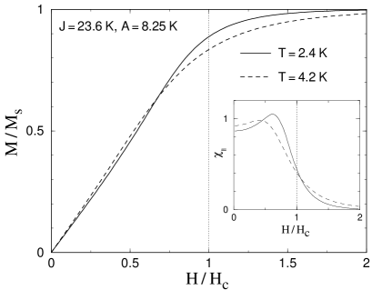
FIG. 9.: TMRG calculation of the field dependence of the magnetization $M$ for a wide field range and two typical values of temperature. The inset displays the corresponding results for the field dependence of the susceptibility. The field is applied along the $c$-axis and the critical field $H_{c}$ is estimated to be $58$ kG for $g_{\parallel}=2.13$.

It is clear that we cannot go farther with our theoretical arguments without explicit knowledge of detailed experimental data on $M(H)$ in this field region. We thus conclude the discussion of magnetization with a comment concerning an apparent contradiction between the results of Fig. 9 and those given earlier in Fig. 8 for lower field strengths. Indeed, Fig. 8 suggests that the magnetization $M(H)$ for any given field $H$ decreases with increasing temperature, as expected, while Fig. 9 indicates that a relative crossing occurs between any two $M(H)$ curves. The resolution of this apparent paradox lies in the fact that the values of temperature employed in Fig. 8 are all greater than the temperature $T\simeq 7.5$ K, at which the maximum of the zero-field susceptibility of Fig. 7 occurs, while those of Fig. 9 are smaller.

Finally, we discuss the specific heat in a field parallel to the $c$-axis. It appears that no measurements have been made for this field orientation but could prove to be feasible in the future.[23] Our TMRG calculation of the excess specific heat is illustrated in Fig. 10 for the two values of temperature employed in our preceding discussion of the magnetization. The characteristic double peak near the critical field $H_{c}$ was anticipated by earlier work [22] based on a classical transfer matrix calculation, on the known exact solution for a spin-$\frac{1}{2}$ XY chain, as well as on an accurate numerical solution for a spin-$\frac{1}{2}$ XXZ chain based on the Bethe Ansatz. The calculated double peak is also a clear departure from the corresponding prediction of the dilute-magnon approximation [22] and could eventually be observed in $\mathrm{CsNiF_{3}}$. An unfortunate feature of Fig. 10 is that a strongly pronounced double peak is predicted to occur in the low-temperature region where the 1D model is no longer applicable.

FIG. 10.: TMRG calculation of the excess specific heat for a wide field range and two typical values of temperature. The field is applied along the $c$-axis and the critical field $H_{c}$ is estimated to be $58$ kG for $g_{\parallel}=2.13$.

IV Conclusion

We have presented a more or less complete calculation of the dynamics and the thermodynamics associated with the spin-$1$ Hamiltonian (1). The $T=0$ dynamics is efficiently described by an $1/n$ expansion whose full potential has not yet been explored. For example, an accurate calculation of the magnon dispersion for a field parallel to the $c$-axis is also possible but has not been carried out mainly because there seems to have been no experimental effort in that direction.

On the other hand, the thermodynamics is calculated by a powerful TMRG method which has opened the way to obtain accurate theoretical predictions for a wide class of quantum magnetic chains. Suffice it to say that our present algorithm may be trivially adjusted to handle spin-$1$ Haldane-gap antiferromagnets in the presence of anisotropy and external fields. Even in the case of completely integrable spin-$\frac{1}{2}$ chains, for which the Bethe Ansatz applies, the calculation of the thermodynamics is far from trivial.[24] Nevertheless, TMRG can be applied in a straightforward manner irrespective of complete integrability.[21]

The extent to which the 1D Hamiltonian (1) may describe the magnetic properties of $\mathrm{CsNiF_{3}}$ has been debated on several occasions. Our calculations confirm the general conclusion that the 1D model accounts for the main features of all available experimental data. But it is also clear that departures from ideal model behavior are present, especially at low temperatures approaching the 3D-ordering transition temperature $T_{N}=2.7$ K.

- [1] Present address: Institute of Theoretical Physics, Chinese Academy of Sciences, Beijing 100080, P.R. China.
- [2] M. Steiner, J. Villain and C. G. Windsor, Adv. Phys. 25, 87 (1976).
- [3] M. Steiner and J. K. Kjems, J. Phys. C : Solid State Phys. 10, 2665 (1977).
- [4] P. A. Lindgard and A. Kowalska, J. Phys. C : Solid State Phys. 9, 2081 (1976).
- [5] T. Delica, W. J. M. de Jonge, K. Kopinga, H. Leschke and H. J. Mikeska, Phys. Rev. B 44, 11773 (1991).
- [6] A. Cuccoli, V. Tognetti, P. Verrucchi and R. Vaia, Phys. Rev. B 46, 11601 (1992).
- [7] N. Papanicolaou, Nucl. Phys. B 240, 281 (1984).
- [8] S. R. White, Phys. Rev Lett. 69, 2863 (1992).
- [9] R. J. Bursill, T. Xiang and G. A. Gehring, J.Phys. : Condens. Matter 8, L583 (1996).
- [10] X. Wang and T. Xiang, Phys. Rev. B 56, 5061 (1997).
- [11] I. Peschel, X. Wang, M. Kaulke and K. Hallberg, Density - Matrix Renormalization , Lecture Notes in Physics, vol. 258 (Springer - Verlag, New York, 1999).
- [12] M. Steiner, private communication.
- [13] J. T. Chui and K. B. Ma, Phys. Rev. B 27, 4515 (1983).
- [14] C. M. Bender and S. A. Orszag, Advanced Mathematical Methods for Scientists and Engineers (McGraw-Hill, New York, 1978).
- [15] L. R. Mead and N. Papanicolaou Phys. Rev. B 26, 1416 (1982).
- [16] G. M. Wysin and A. R. Bishop, Phys. Rev. B 34, 3377 (1986).
- [17] C. Dupas and J - P. Renard, J. Phys. C : Solid State Phys. 10, 5057 (1977).
- [18] A. P. Ramirez and W. P. Wolf, Phys. Rev. B 32, 1639 (1985).
- [19] R. Vaia, private communication.
- [20] J. D. Johnson and J. C. Bonner, Phys. Rev. B 22, 251 (1980).
- [21] X. Wang, X. Zotos, J. Karadamoglou and N. Papanicolaou, Phys. Rev. B 61, 14303 (2000).
- [22] N. Papanicolaou and P. Spathis, Z. Phys. B - Condensed Matter 65, 329 (1987); J. Phys. C. : Solid State Phys. 20, L783 (1987).
- [23] M. Orendac, A. Orendacova and M. W. Meisel, private communication.
- [24] A. Klümper, Z. Phys. B 91, 507 (1993).