Random walks on fractals and stretched exponential relaxation

Abstract

Stretched exponential relaxation ($\exp{-(t/\tau)}^{\beta_{K}}$) is observed in a large variety of systems but has not been explained so far. Studying random walks on percolation clusters in curved spaces whose dimensions range from $2$ to $7$, we show that the relaxation is accurately a stretched exponential and is directly connected to the fractal nature of these clusters. Thus we find that in each dimension the decay exponent $\beta_{K}$ is related to well-known exponents of the percolation theory in the corresponding flat space. We suggest that the stretched exponential behavior observed in many complex systems (polymers, colloids, glasses…) is due to the fractal character of their configuration space.

The stretched exponential decay function, $q(t)=\exp{-(t/\tau)}^{\beta_{K}}$, was initially proposed empirically in 1854 by R. Kohlrausch[1] to parametrise the discharge of Leyden jars, and was rediscovered in 1970 by Williams and Watts[2]. Since then the phenomenological ”KWW” expression has been shown to give an excellent representation of experimental and numerical relaxation data in a huge variety of complex systems including polymers, colloids, glasses, spin glasses, and many more. This behavior has attracted considerable curiosity; it has been discussed principally in terms of models where individual elements relax independently with an appropriate wide distribution of relaxation times (see for instance[3, 4, 5, 6]). However, despite the ubiquity of the KWW expression, in the view of many scientists its status remains that of a convenient but mysterious phenomenological approximation having no fundamental physical justification.
Here we demonstrate that on the contrary KWW is in fact a bona fide and respectable relaxation function; exactly this form of relaxation appears naturally when we consider random walks on fractal structures in closed spaces of general dimensions. We suggest that the physical significance of the relaxation behavior in numerous complex systems should be reconsidered in the light of this result.
For random walks on fractal clusters in Euclidean (flat) spaces, it is well known that if $r(t)$ is the distance of the walker from the starting point after time $t$, then $<r^{2}(t)>\ \propto t^{2/2+\theta}=t^{\beta_{RW}}$[7, 8]. Here $\beta_{RW}=\tilde{d}/D$ where $\tilde{d}$ and $D$ are the spectral and fractal dimensions of the cluster respectively. For a critical percolation fractal, $\theta=(\mu-\beta)/\nu$ where $\mu$, $\beta$ and $\nu$ are universal percolation critical exponents [7, 8] whose numerical values are known quite accurately in all dimensions [9, 10, 11, 12, 13, 14].
For random walks on the surface of a sphere, which is a closed surface, the local behavior $<r^{2}(t)>\ \propto t$ can be shown to lead exactly to an exponential decay of the autocorrelation $<cos(\theta(t))>\propto exp(-t/\tau)$ where $\theta(t)$ is the angle between the initial $t=0$ position vector of the walker and the position vector at time $t$. With an appropriate definition of $<cos(\theta(t))>$ this result holds for hyperspheres in any dimension. For random walks on a percolation fractal inscribed on a closed space with the topology of a hypersphere, it was conjectured some years ago that the end-to-end autocorrelation function should decay as a KWW stretched exponential, with the Kohlrausch exponent $\beta_{K}$ equal to the flat space percolation fractal random walk exponent, i.e. $\beta_{K}=\beta_{RW}$ in any space dimension [15, 16]. This can be understood simply in terms of a ”fractal” time $t^{\beta}_{RW}$ replacing $t$ in both the local $<r^{2}(t)>$ and the exponential $<cos(\theta(t))>$ expressions above. This conjecture has been extensively tested numerically but only in the extreme case of the very high dimensional hypercube [16, 17, 22] (the hypercube has the same closed space topology as a hypersphere). In the present work we have studied numerically the general case of random walks on percolation clusters on hyperspherical surfaces for the range of different embedding dimensions $d$ running from $3$ to $8$.
The simplest case to visualize is the surface of a sphere in dimension $d=3$. The surface is decorated with small disks whose centers are distributed at random. Several clusters, made of overlapping disks, can be determined. The largest cluster contains more and more disks as the total number of disks is increased. Just as there appears a percolation cluster (containing a non-infinitesimal fraction of the total number of disks) for the equivalent system in the two dimensional flat space above a critical value of disk concentration, so the largest cluster “percolates” on the surface of the sphere when the number of disks is sufficiently large. As an illustration, in figure 1, we have represented the two dimensional projection of the percolating cluster in the case $\delta/R=0.01$ (where $\delta$ is the disk diameter and $R$ the sphere radius). Here $N_{p}=179200$ disks have been disposed at random; only the largest cluster, containing 38130 disks, is represented. Note that this cluster spans almost a hemisphere, a situation intermediate between a well localized cluster ($N<<N_{p}$) and a cluster spanning uniformly the whole surface of the sphere ($N>>N_{p}$).
The position of a given disk center can be defined by the $d=3$ coordinates $x_{i}$, where the origin is taken as the center of the sphere. Imagine now a walker jumping at random from one disk center to the center of any disk overlapping it. While the values of the coordinates averaged over many walks $<x_{i}(t)>$ stay finite for $N<<N_{p}$ (the walker is localized) they decay exponentially to zero for $N>>N_{p}$, finally losing memory of their initial values. Of course, in the limit $N>>N_{p}$, $<x_{i}(t)>$ goes to zero since the random walker starts to investigate the largest cluster (which fills uniformly the curved space) entirely. Our calculations show that right at the percolation where the largest cluster is fractal, the decay is critical, and takes up precisely the stretched exponential form, with a $\beta_{K}$ exponent equal to $\beta_{RW}$, already known for the random-walk on a percolating cluster in a two-dimensional flat space. Our calculation is the generalization of this picture over a wide range of dimensions, in particular for dimensions larger than $n=6$, where it is known that $\beta_{RW}$ reaches its mean-field value $1/3$.
Consider the surface of a $d$-dimensional (hyper)sphere of unit radius which can be defined, using Euclidean coordinates, by $\sum_{i=0}^{d}x_{i}^{2}=1$. This (hyper)surface is a closed and curved $n$-dimensional ($n=d-1$) space, $S_{n}$, on which one can define a geodesic distance between two points (1) and (2) by $\theta=\cos^{-1}q$ where $q$ is the scalar product of the end positions, i.e. $q={\bf r}_{1}.{\bf r}_{2}=\sum_{i=0}^{d}x_{i}^{(1)}x_{i}^{(2)}$. Of course, this distance becomes asymptotically equivalent to the Euclidean distance in the limit of distances infinitesimally small compared to the radius of the (hyper)sphere (which is here set to unity). On this $n$-dimensional (hyper)surface, identical $n$-dimensional small (hyper)disks (called disks in the following) of diameter $\delta<<1$ are disposed sequentially, the successive disk centers being chosen at random uniformly on $S_{n}$. To determine the cluster structure, as soon as a new disk is added, a search for connections with previous disks is performed by checking if their center-to-center geodesic distance is smaller than $\delta$. At each stage, when $N$ disks have been disposed on $S_{n}$, we can define and label the different clusters made up of connected disks. In particular one can determine the largest cluster containing the greatest number $N_{m}$ of disks. Also one can characterize the overall filling of the space by a dimensionless parameter $\eta$, ratio between the sum of the area of the individual disks and the total area of $S_{n}$ [21]. Note that this filling parameter is larger than the true volume fraction $c$, because of multiple counting due to overlaps, and therefore $\eta$ can eventually exceed unity. More precisely it has been shown that $c=1-\exp{(-\eta)}$[18, 19]. Percolation occurs for $\eta$ larger than a threshold value $\eta_{p}$ above which $P=N_{m}/N$, which measures the probability for a given disk to belong to the largest cluster, remains non-zero in the thermodynamic limit $\delta\rightarrow 0$. In practice the curve $P(\eta)$ exhibits a sigmoïdal shape which becomes sharper and sharper at $\eta_{p}$ as $\delta\rightarrow 0$.
Once the largest cluster has been identified, we choose one of its constitutive disk centers ${\bf r}(0)$ at random as a starting point. We perform a random walk on the cluster by performing successive jumps, first from ${\bf r}(0)$ to the center ${\bf r}(1)$ of any other disk connected to it (chosen at random over all its overlapping disks), then iterating from ${\bf r}(1)$ to ${\bf r}(2)$, etc..[20] After t steps, the “correlation function” ${\bf r}(0).{\bf r}(t)$ is calculated. This is the scalar product of the two end positions, which is no more than the cosine of the geodesic end-to-end distance $\theta$ measured on $S_{n}$. In practice we calculate the quantity $q(t)=<\cos\theta>$ which has been averaged, for a given number of steps $t$, over $N_{r}$ independent realizations of the largest cluster as well as over $N_{s}$ independent choices of the starting point on each cluster. Given dimension $n$ and size $\delta$, the behavior of $q(t)$ has been analyzed for different filling values $\eta$.
An example with $n=3$ and $\delta=0.02$ is shown in figure 2, where $-\ln|q(t)|$ has been plotted as a function of $t$ in a log-log plot, after taking an average over independent walks starting from $N_{s}=10500$ different disks on each of the $N_{r}=20$ independently generated largest clusters (a typical value of the number of disks in the percolating cluster is $N_{m}\simeq 700000$).
If the relaxation function $q(t)$ is strictly a stretched exponential, this type of plot produces a straight line of slope $\beta_{K}$. For the critical value of $\eta$ (here $\eta_{p}\simeq 0.3452$), one observes a clear straight line behavior in the numerical data over (at least) six decades in $t$ (the walk for $\eta_{p}$ has been extended to illustrate this point). In the inset, we show how we estimate $\eta_{p}$ and $\beta_{K}$. The effective slope of the log-log plot has been determined by a least-square fit within an interval of one-tenth of the total range in $\ln t$ and plotted as a function of $\ln t$. The percolation threshold $\eta_{p}$ is estimated as the $\eta$-value giving the widest plateau at large times, and the $\beta_{K}$ exponent is taken as this plateau value. This procedure has been repeated for different values of $\delta$ and for dimensions $n$ ranging from 2 to 7 (for $n$=1 it is well known that the percolation transition does not occur [11]). The lowest attainable $\delta$ values are mainly determined by the limited memory of our computers. In practice the values of $N_{s}$ have been chosen to be of the order of two percent of $N_{m}$, and $N_{r}$ has been chosen so as to obtain runs of the order of a day on regular high speed PC computers. $N_{s}$ varies from few thousands to a few units when decreasing $\delta$ from about 0.3 to its lowest attainable $\delta$ value. This protocol leads to error bars of the order of 0.01 for the exponent estimates. Of course the “true” values of the percolation thresholds and exponents are obtained by an extrapolation to the ”thermodynamic” limit $\delta\rightarrow 0$.
The numerical results for $\eta_{p}$ in $n=2$ and $3$ are in excellent agreement with accurate estimates from flat space calculations [18, 19], and $\eta_{p}$ drops quasi-exponentially with $n$ for higher dimensions. The data for $\beta_{K}$ are summarized in figure 3, where $\beta_{K}$ has been plotted as a function of $\delta$. On the $\delta=0$ axis of figure 3, we have indicated the best estimates of the flat space $\beta_{RW}$ with their associated error bars, calculated from recent $\mu$, $\beta$ and $\nu$ values available in the literature [9, 10, 11, 12, 13, 14]. We note that for all $n\geq 6$, $\beta_{RW}=1/3$ exactly, since $n=6$ is the upper critical dimension for percolation[11]. It is quite remarkable that for each dimension $n$, a simple straight line fit of our data goes through the corresponding $\beta_{RW}$ value to within the numerical error or, at least, extrapolates to a value very close to it.
It should be noticed that the law $<\cos\theta>\propto\exp{-(t/\tau)^{\beta_{K}}}$ not only contains the large time relaxation behavior but also the short time behavior as, after expanding both sides for small $t$ and $\theta$, it becomes $<\theta^{2}>\propto(t/\tau)^{\beta_{K}}$. Since for short times the random walker stays on a $n$-dimensional surface tangent to the (hyper)sphere, one recovers the law $<r^{2}>\propto t^{\beta_{RW}}$ in dimension $n$. This could explain why the stretched exponential behavior extends over so large a region of time (see figure 2). In practice, as in flat space, at very short times there are corrections to scaling due to the discrete character of the walk.
These data can be taken as a clear numerical demonstration that random walks on a fractal cluster inscribed on a hypersphere in any dimension lead necessarily to a stretched exponential decay of the correlation function, with a Kohlrausch exponent $\beta_{K}$ equal to the ratio ${\tilde{d}}/D$ of the spectral and fractal dimensions of the cluster. Thus the stretched exponential relaxation on a fractal in a closed space appears as the precise analogue of the sub-linear diffusion on a fractal in a flat space.
Why is this relevant to relaxation in complex systems ? A complex system is made up of many individual elements (atoms, molecules, spins,…etc), all in interaction with each other. The total space of all possible configurations of the whole system is a huge closed space having a very high dimension, of the order of the number of elements. These spaces are so astronomically large that an explicit evaluation of their properties, configuration by configuration, is almost impossible except for tiny systems. Each configuration has an energy associated to it. At finite temperature $T$ only a restricted subset of configurations are of low enough energy to be thermodynamically accessible by the system. In equilibrium at $T$ above any ordering temperature, the system is permanently exploring all this subset of accessible configurations by successive movements or reorientations of local elements of the total system. By definition this equilibrium relaxation can be mapped onto a random walk of the point representing the instantaneous configuration of the total system within the space of accessible configurations. Thus the configuration space of a complex system can be viewed as a “rough landscape”. In such a scenario, the portion of configuration space available to the system consists of only a restricted set of tortuous configuration space paths. In this situation, when real measurements are made, the observed relaxation functions must reflect the complex morphology of the available configuration space, and so will be slow and non-exponential - typically stretched exponential. Now, any relaxation function including the KWW function can be represented as the sum of an appropriate distribution of elementary exponential relaxations. However it is important to note that the independent exponentially relaxing elements in a complex system are the modes of the whole system not the atoms, molecules or spins which are in strong interaction with each other[22]. It is the morphology of the configuration space which determines the mode distribution and the form of the relaxation.
We have just seen that a closed space fractal structure necessarily leads to a relaxation process which is exactly of stretched exponential type; we suggest that, inversely, when a complex system at temperature $T$ is actually observed to relax with a stretched exponential, it is the signature of a fractal morphology of the available configuration space at that temperature. In particular, whatever the microscopic details of the interactions in a glass former are, it is generally observed that as the glass temperature is approached from above, KWW relaxation sets in. The implication is that phase space takes up a fractal morphology as a consequence of the intrinsic complexity associated with glassiness. The image of the glass transition which follows is that of a percolation transition in phase space[15, 22] with the temperature being analog to the filling parameter. As would be expected from the argument given above, the Kohlrausch exponent is observed to tend to a limiting value of $1/3$ as the glass transition is approached in a number of systems, [23, 24, 25, 26] for instance.
In summary, we have demonstrated that random walks on fractals in closed spaces give stretched exponential relaxation, and we suggest that stretched exponential relaxation is ubiquitous in nature because configuration spaces are fractal in many complex systems.

 

FIG. 1.: Two-dimensional projection of a typical percolating cluster of disks of diameter $\delta=0.01$ on the surface of a sphere of unit radius. Here $N_{p}=179200$ disks have been disposed at random; only the largest cluster, containing $N_{m}=38130$ disks, is represented.

FIG. 2.: Plot of $-\ln|q(t)|$ versus t (averaged over $N_{r}=20$ and $N_{s}=10500$) for $n=3$, $\delta=0.02$ and for different $\eta$ values: from bottom to top $\eta=$ 0.335, 0.34, 03452, 0.35, 0.355 (the statistical error bars do not exceed the thickness of the lines). In inset the local value of the exponent $\beta$ is plotted as a function of $\ln t$ for the different $\eta$ values in order to estimate $\eta_{p}$ and $\beta_{K}$.

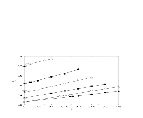
FIG. 3.: Variation of the exponent $\beta_{K}$ as a function of the (hyper)disk diameter $\delta$ for dimension $n=2,3,4,5,6$ and $7$ (from top to bottom). The solid lines represent least square linear fits of the data points. The best estimates of the flat space exponent $\beta_{RW}$ with their associated error bars [9-14] are represented by the stars on the y axis.

REFERENCES

- [1] R. Kohlrausch, Pogg. Ann. Phys. Chem. 91, 179 (1854). The frequently quoted Kohlrausch paper published in 1847 does not mention stretched exponentials.
- [2] G. Williams, D.C. Watts, Trans. Faraday Soc. 66, 80 (1970).
- [3] R.G. Palmer, D.L. Stein, E. Abrahams, P.W. Anderson, Phys. Rev. Lett. 53, 958 (1984).
- [4] H. Sher, M.F. Schlesinger, J.T. Bendler, Physics Today 44, 26 (1991).
- [5] J.C. Phillips, Rep. Prog. Phys. 59, 1133 (1996).
- [6] A. Bunde, S. Havlin, J. Klafter, G. Gräff, A. Shehter, Phys. Rev. Lett. 78, 3338 (1998).
- [7] S. Alexander, R. Orbach, J. Physique Lett. 43, L625 (1982).
- [8] Y. Gefen, A. Aharony, S. Alexander, Phys. Rev. Lett. 50, 77 (1983).
- [9] J. Adler, Y. Meir, A. Aharony, A.B. Harris, Phys. Rev. B 41, 9183 (1990).
- [10] J. Adler, Y. Meir, A. Aharony , L. Klein, J. Stat. Phys. 58, 511 (1990).
- [11] D.Stauffer , A. Aharony, An Introduction to Percolation theory,Taylor and Francis (London) 1994.
- [12] H.G. Ballesteros, L.A. Fernandez, V. Martin-Mayor, A.M. Sudupe, G. Parisi and J.J. Ruiz-Lorenzo, J. Phys. A 32, 1 (1999).
- [13] H.G. Ballesteros, L.A. Fernandez and J.J. Ruiz-Lorenzo, Phys. Lett. B 400, 346 (1997).
- [14] C.D. Lorenz, R.M. Ziff, Phys. Rev. E 57, 230 (1998).
- [15] I.A. Campbell, J.Phys. (France) Lett. 46, L1159 (1985).
- [16] I. A. Campbell, J.M. Flesselles, R. Jullien, R. Botet, J. Phys. C 20, L47 (1987).
- [17] N. Lemke, I. A. Campbell, Physica A 230, 554 (1996).
- [18] J. Quintinilla, S. Torquato and R. M. Ziff, J. Phys. A. (to be published)
- [19] M.D. Rintoul and S. Torquato, J. Phys. A 30, L585 (1997).
- [20] Note that the jump lengths are uniformly distributed between 0 and . It is a well known result of the percolation theory that the precise form of the length distribution (as soon as it is bounded) is irrelevant for the determination of the critical exponents.
- [21] is defined by where is the area of a (hyper)disk of radius . Using standard algebra, one gets with
- [22] R.M.C. de Almeida, N. Lemke, I.A. Campbell, cond-mat/0003351.
- [23] A.T. Ogielski, Phys. Rev. B 32, 7384 (1985).
- [24] E. Bartsch, M. Antonietti, W. Schupp, and H. Sillescu, J. Chem. Phys. 97, 3950 (1992).
- [25] L. Angelani, G. Parisi, G. Ruocco and G. Vilani, Phys. Rev. Lett. 81, 4648 (1998).
- [26] A.Alegría et al, Macromolecules 28, 1516 (1995).