[

Macroscopic Manifestation of Microscopic Entropy Production: Space-Dependent Intermittence

Abstract

We study a spatial diffusion process generated by velocity fluctuations of intermittent nature. We note that intermittence reduces the entropy production rate while enhancing the diffusion strength. We study a case of space-dependent intermittence and prove it to result in a deviation from uniform distribution. This macroscopic effect can be used to measure the relative value of the trajectory entropy.

]

The problem of detecting the macroscopic effects of microscopic randomness has been an active field of research for several years. The literature is so extended that we limit ourselves to only a few sample papers[1, 2, 3, 4, 5]. The problem is hard and controversial. It is possible to derive the ordinary diffusion equation, often used in these studies, as the asymptotic limit of a dynamic prescription with no irreversibility ingredients[6], thereby raising the problem itself of where to locate the source of entropy production. This source is often identified with the random nature of the microscopic trajectories, which, at least in principle, is rigorously defined by the Kolmogorov-Sinai (KS) entropy $h_{KS}$[7]. Gaspard and Nicolis[1] pointed out that the transport coefficients of open systems, and notably the diffusion coefficient, can be expressed as the difference between the positive Lyapunov exponent and the KS entropy, thereby implying that the macroscopic manifestation of the trajectory randomness has to be looked for in non-equilibrium processes, in line with the tenets of irreversible thermodynamics[8].

Here we discuss a different way to the macroscopic manifestation of the trajectory entropy, based on the diffusion of a space variable $x$ collecting the intermittent fluctuations of a random velocity $\xi$. We show that in the case where the velocity intermittence is space dependent, the equilibrium reached by the system is the same as that produced by a temperature gradient, even if the kinetic energy of a single trajectory remains rigorously constant throughout the whole observation process. Thus, a “paradoxical” equilibrium distribution shows up, reminiscent of the dynamical Maxwell’s Demon effect, recently discussed by Zaslavsky[9]. This effect is anomalous but is not unphysical, and we show that it can be used to establish the relative value of trajectory entropy.

The velocity $\xi$ is a dichotomous variable, namely, with only two values, $+W$ or $-W$, and we set these values in sequence as follows. We randomly draw integer numbers $l$, interpreted as time lengths in units of $\tau$. We use a random number generator, assumed to draw with uniform probability the numbers $s$ of the interval $[0,1]$. After any drawing we associate the selected number $s$ to $y=-(1/\lambda)\ln s$. Then we consider only the integer part of it, $l=[y]+1$. The probability of large $l$’s is so high that we can adopt a continuous rather than a discrete picture, for both the interval lengths, $l$, and the time associated to them, $t=l\tau$. The probability of drawing the time $t$ is proportional to:

$$\psi(t)=\frac{\lambda}{\tau}\exp\left(-\frac{t}{\tau}\lambda\right).$$ (1)

Adopting the jargon of the authors of Ref.[10], who used intermittently chaotic maps to derive faster than normal diffusion, we refer to $\psi(t)$ as the waiting time distribution of the laminar phase. This means that the $i$-th drawing selects the integer number $l(i)$, which defines a time interval $l(i)\tau$ corresponding to the velocity $\xi$ maintaining the value $+W(-W)$, without changing sign. At the $(i+1)$-th step, when the length $l(i+1)$ is selected, the velocity $\xi$ changes sign and keeps the new value $-W(+W)$ for the whole interval of time $l(i+1)\tau$. There is no uncertainty associated with the choice of the velocity sign. Randomness is involved only at the moment of drawing the number $s$. We call $H(E)$ the entropy increase associated with this drawing. This quantity is assumed to be the same for any drawing, and, consequently, as we shall see, the Maxwell’s Demon effect is independent of it. It is evident that the sequence of symbols $\xi(t)$ generated by this procedure is characterized by the steady rate of entropy increase

$$h_{E}=H(E)\frac{\lambda}{\tau},$$ (2)

since $\tau/\lambda$ is the mean time spent by the velocity in the laminar phase. We refer to this entropy as External (E) entropy to point out that it does not coincide with the KS entropy.

What about the connection between the KS and the E-entropy? This question can be answered considering the asymmetric Bernoulli map studied by Dorfmann et al. [11]. We describe this map, changing the notations of Ref.[11], as follows. We consider the variable $z$, moving in the interval $[0,1]$, with the condition of folding back into this interval the portion of $z$ exceeding the value $z=1$, and with the following dynamic recipe:

$$z_{n+1}=z_{n}/q,$$ (3)

for $0\leq z_{n}<q$, and

$$z_{n+1}=(z_{n}-q)/p,$$ (4)

for $q\leq z_{n}<1$. We assume $q=1-p$ and we consider this map in the case where $p<<1$. This means that the KS entropy of this map[11],

$$h_{KS}=(1-p)\ln\left(\frac{1}{1-p}\right)+p\ln\left(\frac{1}{p}\right),$$ (5)

becomes (using a time step $\tau$, not necessarily equal to $1$)

$$h_{KS}=\frac{p}{\tau}\left[1+\ln\left(\frac{1}{p}\right)\right].$$ (6)

Let us assign the symbol $+W$ to the “laminar” region of Eq. (3) and the symbol $-W$ to the “chaotic” region of Eq. (4). The resulting sequence is apparently different from that produced by the prescription earlier adopted to generate the fluctuations of the variable $\xi$. However, the numerical calculation proves that in the limiting case $p<<1$ the two kinds of symbolic sequences yield the same KS entropy[12]. The reader can easily convince him/herself that the two KS entropies are identical by noticing that the only element of randomness concerns the prediction about the time duration of the laminar phase. The distribution of the laminar phase waiting times is given by Eq.(1) with $\lambda=p/(1-p)$. The KS entropy can be written in a form reminiscent of that of the E-entropy of Eq. (2),

$$h_{KS}=H(KS)\frac{\lambda}{\tau},$$ (7)

provided that the uncertainty $H$ is now defined as

$$H(KS)\equiv\left(\frac{\lambda}{1+\lambda}\right)\left[1+\ln\left(\frac{1+\lambda}{\lambda}\right)\right].$$ (8)

The source of uncertainty is the same as that mirrored by the E-entropy, namely, the random drawing of numbers of the interval $[0,q]$, which, in fact, in the limiting case of $p\rightarrow 0$ coincides with the interval $[0,1]$. However, the KS entropy reflects also the fact that the random selection of these numbers is operated by the chaotic region of Eq.(4). The E-entropy, on the contrary, interprets the sporadic randomness as produced by an external source (hence the term external used to denote it) with a strength independent of $\lambda$.

The diffusing variable is the space variable $x(t)$ that in the case when $t/\tau>>1$ can be related to the velocity $\xi(t)$ by

$$x(t)=\int_{0}^{t}\xi(t^{\prime})dt^{\prime}+x(0).$$ (9)

In the special case we are considering, the variable $\xi(t)$ is dichotomous, thereby implying the property

$$\langle\xi(t_{1})\xi(t_{2})\ldots\xi(t_{2n-1})\xi(t_{2n})\rangle=~{}~{}~{}~{}~{}~{}~{}~{}~{}~{}$$ (10)

$$\langle\xi(t_{1})\xi(t_{2})\rangle\ldots\langle\xi(t_{2n-1})\xi(t_{2n})\rangle,$$ (11)

the correlation functions with odd numbers of times vanishing as a consequence of the assumption made that no bias exists, namely, $\langle\xi(t)\rangle=0$. In this condition, it is straightforward to prove that for $1\leq n$

$$\langle x^{2n}(t)\rangle=(2n)!W^{2n}\int_{0}^{t}dt_{1}\int_{0}^{t_{1}}dt_{2}\ldots\times~{}~{}~{}~{}~{}~{}$$ (12)

$$\int_{0}^{t_{2n-1}}dt_{2n}\Phi_{\xi}(t_{1}-t_{2})\ldots\Phi_{\xi}(t_{2n-1}-t_{2n}),$$ (13)

where $\Phi_{\xi}(t)$ denotes the normalized correlation function of $\xi$ ($\Phi_{\xi}(0)=1$). It is also straightforward to show that the Liouville-like equation, generating all the moments of Eq. (13), and thus properly describing this diffusion process, is:

$$\frac{\partial}{\partial t}\sigma(x,t)=W^{2}\int_{0}^{t}\Phi_{\xi}(t-t^{\prime})\frac{\partial^{2}}{\partial x^{2}}\sigma(x,t^{\prime})dt^{\prime}.$$ (14)

On the other hand, although this equation is expected to be an exact picture of the dichotomous process under study, it can also be derived, via a projection procedure, from a standard Liouville picture applied to an additional set of variables, ${\bf\Psi}$, responsible for the random-like behavior of the variable $\xi$[13], as well as to $x$, $\xi$. We note that in the asymptotic time limit this equation, under the assumption alone that the correlation function $\Phi_{\xi}(t)$ is integrable, yields the ordinary diffusion equation

$$\frac{\partial}{\partial t}\sigma(x,t)=D\frac{\partial^{2}}{\partial x^{2}}\sigma(x,t).$$ (15)

Using the proper connection between $\psi(t)$ and $\Phi_{\xi}(t)$[13, 14, 15], we express the diffusion coefficient as

$$D=W^{2}\frac{\tau}{2\lambda}.$$ (16)

It is embarrassing, in our opinion, that the same result as that produced by the random microscopic trajectory here under study, the ordinary diffusion equation of Eq. (15), can be derived from a perspective with no explicit use of microscopic randomness [6], hence keeping alive the long standing debate on the origin of thermodynamics and statistical mechanics that, according to Boltzmann[16] rests on the key action of infinitely many degrees of freedom. This is probably the strength of statistical mechanics, whose successes rest on fundamental equations, such as the Fick’s law[6], independent of the philosophical perspective adopted for their derivation. Here, we prove that microscopic randomness can produce ostensible macroscopic effects. This raises the interesting issue of how to derive these effects from within the deterministic perspective[6, 16].

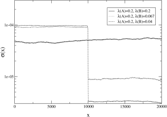
FIG. 1.: Typical equilibrium distributions.

We have seen that $1/\lambda$ is the time dilatation intensity. The parameter $\lambda$, consequently, measures the intermittence-induced reduction of entropy production. To prove how a form of anomalous statistical mechanics can emerge out of this property, let us consider the case where the particle moves in the interval $[0,L]$. In the case of ordinary statistical mechanics, the system of diffusing particles, after a fast transient process reaches a condition of uniform equilibrium distribution, thereby opening a temporary window for the observation of entropy production, which, in fact, from the pioneer times of Ref.[8] to these days[3], is done in out of equilibrium conditions. Here we draw benefits from the intermittent nature of the microscopic process, controlled by $\lambda$. We call $A$ and $B$ the left and right portion of the container, and we assign different values of $\lambda$ to them, while leaving the kinetic energy constant. The time dilatation in $A$ is smaller than in $B$, namely, $\lambda(A)>\lambda(B)$. At the moment of the $j$-th drawing, the number $s(j)$ generates either $y(j)=-(1/\lambda(A))\ln s(j)$ or $y(j)=-(1/\lambda(B))\ln s(j)$, according to whether the particle is in $A$ or $B$ at the end of the earlier laminar phase. At $x=0$ and $x=L$, the velocity $\xi$ changes signs, so as to mimic the elastic collision with the walls, and keeps it till to exhaust the sojourn time selected by the last drawing. According to Eq. (16), the diffusion process in $A$ is slower than in $B$, thereby making, as shown by Fig. 1, $\sigma(A)>\sigma(B)$, where $\sigma(A)$ and $\sigma(B)$ are the particle densities in $A$ and $B$, respectively. On the basis of the earlier theoretical arguments, it is evident that this Maxwell’s Demon effect[9] is determined by the fact that the trajectory entropy in $A$ is larger than in $B$.

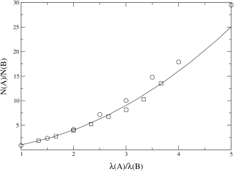
FIG. 2.: Ratio between equilibrium populations in the two half spaces, as function of the lifetimes ratio. Solid line is theory, circles are simulation results based on the integration of a single random trajectory, squares are simulation results based on the long time distribution obtained evolving an initially flat distribution.

In fact, the numerical experiment proves that (Fig. 2)

$$N(A)/N(B)=[h_{E}(A)/h_{E}(B)]^{2},$$ (17)

where $N(A)$ and $N(B)$ denote the number of particles in $A$ and $B$, respectively, and $h_{E}(A)$ and $h_{E}(B)$ are the corresponding external entropies. This numerical result can be given a plausible theoretical explanation. We note that the traditional diffusion equation of Eq. (15) is a proper description of the diffusion process in a time scale larger than $\tau/(2\lambda)$. This observation yields the following balance equation, between $\sigma(A)$ and $\sigma(B)$,

$$D(A)\sigma(A)\Delta(A\rightarrow B)=D(B)\sigma(B)\Delta(B\rightarrow A),$$ (18)

where $D(A)$ and $D(B)$ denote the diffusion coefficients of $A$ and $B$, respectively, evaluated according to the prescription of Eq. (16). The rationale for this key balance is that, according to the theory of the first passage time[17], the diffusion coefficients $D(A)$ and $D(B)$ can be interpreted as the rate of the processes of diffusion from the walls at $x=0$ and $x=L$, respectively, to the border between the two portions. Thus the number of particles entering the portion $B$, per unit of time, $N(A\rightarrow B)$, is proportional to $D(A)$. However, the larger is the memory of the initial condition, the larger is the number of particles moving from $A$ to $B$. Thus, $N(A\rightarrow B)$ must be proportional also to a spatial window of size $\Delta(A\rightarrow B)$. Similar arguments are used for $N(B\rightarrow A)$, and Eq. (18) follows. It is natural to assume $\Delta(A\rightarrow B)$ and $\Delta(B\rightarrow A)$ to be proportional to $W\tau/\lambda(A)$ and $W\tau/\lambda(B)$, respectively. This assumption, Eq. (16) and Eq. (18) yield a theoretical prediction coinciding with Eq. (17).

In conclusion, $h_{E}$, as well as $h_{KS}$, is a form of trajectory entropy, difficult to detect from within a macroscopic equilibrium condition. We have proved that the space dependent intermittence yields unusual, but not unphysical, macroscopic equilibrium properties that can be used to measure the relative value of the E-entropy, and, hence, through the relations between the E-entropy and the KS entropy, established in this letter, to derive also information on the KS entropy. The Maxwell’s Demon effect of this letter is similar to that of Zaslavsky, but not identical to it. As shown by Zaslavsly[18], in his model the left container, corresponding to the portion $A$, is a Cassini billiard and the right container, corresponding to the portion $B$, is a Sinai billiard. The larger density in $A$ is not caused by a slower diffusion, but by a more extended sojourn time in the state of regular collisions with the walls (the laminar state of the Zaslavsky model). However, we are convinced that by properly adapting to that case the perspective established in this letter, it should be possible to express also the Zaslavsky version of the Maxwell’s Demon effect as a measure of the relative value of the trajectory entropy. In that case the randomness associated to the collision between particle and scatterer is made sporadic by long sojourns in states corresponding to regular collisions with the walls of the container.

Finally, we like to address the connection between the dynamic systems of this letter and the bona fide turbulent process[19], and also the related problem of the thermodynamic nature of a Lévy gas. The inverse power law character of the waiting time distribution is essential to produce the macroscopic manifestation of microscopic intermittence, under the form of anomalous diffusion. The Maxwell’s Demon effect, on the contrary, does not require the waiting time distribution to have an inverse power law nature. As shown in this letter, this form of macroscopic manifestation of intermittence only requires the random bursts to occur with a space-dependent frequency. In fact, the time dilatation strength used in this letter is not constant, and $1/\lambda(A)<1/\lambda(B)$. On the other hand, the exponential condition used in this letter is not necessary: The important property behind the Maxwell’s Demon effect is that the mean sojourn time in the laminar region changes with moving from one to the other portion of the container, including the possibility of being infinite in one of the two portions. Thus, our approach can be easily extended to the case of inverse power law: It is enough to take[20] $y=T[1/(1-s)^{1/(\mu-1)}-1]$. The mean waiting time of the resulting distribution is not affected by the transition from the Gauss to the Lévy statistics, occurring at $\mu=3$, and it keeps a finite value in the whole interval $[2,3]$, but at $\mu=2$, where it diverges. This divergence signals a transition to a non-stationary condition, incompatible with the dynamic derivation of Lévy statistics[21]. This phase transition makes the E-entropy, and with it the KS entropy[22], vanish for $\mu\leq 2$. Thus, this letter suggests that the temperature of a Lévy process becomes infinite at the onset of this transition.

REFERENCES

- [1] P. Gaspard and G. Nicolis, Phys. Rev. Lett. 65, 1693 (1990).
- [2] V. Latora and M. Baranger, Phys. Rev. Lett. 82, 520 (1999).
- [3] T. Gilbert, J. R. Dorfman and P. Gaspard, Phys. Rev. Lett. 85, 1606 (2000).
- [4] W. H. Zurek and J. P. Paz, Phys. Rev. Lett. 72, 2508 (1994).
- [5] A. K. Pattanayak, Phys. Rev. Lett. 83, 4526 (1999).
- [6] M. H. Lee, Phys. Rev. Lett. 85, 2422 (2000).
- [7] J. R. Dorfman, An Introduction to Chaos in Nonequilibrium Statistical Mechanics, Cambridge Lecture Notes in Physics (Cambridge University Press, Cambridge, 1999).
- [8] S. R. de Groot and P. Mazur, Nonequilibrium Thermodynamics (Dover, New York, 1984).
- [9] G. M. Zaslavsky, Physics Today 52(8), 39 (1999).
- [10] T. Geisel, J. Nierwetberg and A. Zacherl, Phys. Rev. Lett. 54, 616 (1985).
- [11] J. R. Dorfman, M. H. Ernst and D. Jacobs, J. Stat. Phys. 81, 497 (1995).
- [12] P. Grigolini, M. G. Pala and L. Palatella, in cond-mat/0007323.
- [13] P. Allegrini, P. Grigolini and B. J. West, Phys. Rev. E 54, 4760 (1996).
- [14] G. Zumofen and J. Klafter, Phys. Rev. E 47, 851 (1993).
- [15] Using the prescription of Ref.[14], it is straigthforward to replace the process with alternated velocity signs, studied in this letter, with an equivalent process, with randomly selected velocity signs, of which Ref.[13] affords an exact treatment.
- [16] J. L. Lebowitz, Physica A 263, 516 (1999).
- [17] C. W. Gardiner, Handbook of Stochastic Methods, Second Edition (Springer, Stuttgart, 1985).
- [18] G. M. Zaslavsky, Physics of Chaos in Hamiltonian Systems (Imperial College Press, London, 1998).
- [19] U. Frisch, Turbulence, the legacy of A. N. Kolmogorov (Cambridge University Press, Cambridge, 1995).
- [20] M. Buiatti, P. Grigolini and L. Palatella, Physica A 268, 214 (1999).
- [21] R. Bettin, R. Mannella, B. J. West and P. Grigolini, Phys. Rev. E 51, 212 (1995).
- [22] P. Gaspard and X.-J. Wang, Proc. Natl. Acad. Sci. USA 85, 4591 (1988).