Edwards’ measures: a thermodynamic construction for dense granular media and glasses

Abstract

We present numerical support for the hypothesis that macroscopic observables of dense granular media can be evaluated from averages over typical blocked configurations: we construct the corresponding measure for a class of finite-dimensional systems and compare its predictions for various observables with the outcome of the out of equilibrium dynamics at large times. We discuss in detail the connection with the effective temperatures that appear in out of equilibrium glass theories, as well as the relation between our computation and those based on ‘inherent structure’ arguments. A short version of this work has appeared in Phys. Rev. Lett. 85, 5034 (2000), cond-mat/0006140.

]

I introduction

Granular systems [5, 6] involve many particles, so there is a strong motivation to treat them with thermodynamic methods. This approach is justified when one is able to identify a distribution that is left invariant by the dynamics (e.g. the microcanonical ensemble), and then assume that this distribution will be reached by the system, under suitable conditions of ’ergodicity’. Unfortunately, because energy is lost through internal friction, and gained by a non-thermal source such as tapping or shearing, the dynamical equations do not leave the microcanonical or any other known ensemble invariant. Moreover, just as in the case of aging glasses, the compaction dynamics does not approach any stationary state on experimental time scales.

Consider a compaction experiment, in which we subject a granular system to gentle, periodic tapping. To keep the discussion simple, we can assume that there is no gravity, and that there is a piston applying a constant pressure on the surface. The system compactifies very slowly [7], in practice never reaching the most dense, optimal packing. At a given long time, when the system has density $\rho(t)$, we may wish to measure for example the fraction of grains that are at relative distance $r$: the structure factor. This quantity being averaged over all particles, one can expect it to be a reproducible observable. However, there is in principle no method to calculate the structure factor other than solving the dynamics.

Some years ago Edwards [8, 9, 10] proposed that one could reproduce the observables attained dynamically by calculating the value they take in the usual equilibrium distribution at the corresponding volume, energy, etc. but restricting the sum to the ‘blocked’ configurations defined as those in which every grain is unable to move. In the case of the previous paragraph, we would compute the structure factor in all the possible blocked configurations of density $\rho(t)$, and calculate the average. Thus, the only input from dynamics would be $\rho(t)$, apart from which the calculation is based on a statistical ensemble.

This ‘Edwards ensemble’ leads immediately to the definition of an entropy (in the glass literature a ‘complexity’) $S_{edw}$, given by the logarithm of the number of blocked configurations of given volume, energy, etc., and its corresponding density $s_{edw}\equiv S_{edw}/N$. Associated with this entropy are state variables such as ‘compactivity’ $X_{edw}^{-1}=\frac{\partial}{\partial V}S_{edw}(V)$ and ‘temperature’ $T_{edw}^{-1}=\frac{\partial}{\partial E}S_{edw}(E)$.

Recent developments in glass theory, especially those related to their out of equilibrium dynamics, have come to clarify and support such a hypothesis — at least within mean-field models (see below). The present paper addresses the natural question of whether Edwards’ measure gives good results for the compaction of finite dimensional, non mean-field models. The result is that there is a class of models for which this is the case. A shorter version of this work has been published in [11].

The article is organized as follows: we first discuss the nature of the assumptions (Subsection I-A), and the evidence in support coming from mean-field models (Subsection I-B). In subsection I-C we discuss in detail the checks already made with Lennard-Jones glasses, in the context of the so-called ‘inherent structures’, and their relation with the present approach.

In sections II and III we treat two finite-dimensional models which reproduce many of the features of glasses and granular media, namely the Kob-Andersen (KA)[13] and Tetris [14] models. We devise a method to count and calculate averages over the blocked configurations, explicitly constructing in this way Edwards’ measure. We compare expectation values thus obtained with equilibrium values and with the outcome of slow, aging dynamics and find very good agreement between the predictions of Edwards’ measure and aging dynamics.

In order to show that this agreement does not hold for all forms of slow dynamics, we repeat the procedure in section IV for another model exhibiting slow, logarithmic relaxations, the random field Ising model (RFIM) [15]. We conclude with a discussion of our results in section V.

A The Assumption

One possibility of making an assumption à la Edwards would be to consider a fast quench, and then propose that the configuration reached has the macroscopic properties of the typical blocked configurations. This would imply that the system stops at a density for which the number of blocked configurations is maximal. We do not follow this path, as we will give sufficient evidence that generically the vast majority of the blocked configurations are much less compact than the one reached dynamically, even after abrupt quenches.

Our strategy here is instead to quench the system to a situation of very weak but non-zero tapping, shearing or thermal agitation. In this way, the system keeps compactifying, albeit at a very slow rate. In this context, we consider a flat measure over blocked configurations conditioned to having the energy and/or density of the dynamical situation we wish to reproduce. This means that we have given up trying to predict the dynamical energy or density by methods other than the dynamics itself.

That configurations with low mobility should be relevant in a jammed situation is rather evident, the strong hypothesis here is that the configurations reached dynamically are the typical ones of given energy and density. Had we restricted averages to blocked configurations having all macroscopic observables coinciding with the dynamical ones, the construction would exactly, and trivially, reproduce the dynamic results. The fact that conditioning averages to the observed energy and density suffices to give, at least as an approximation, other dynamical observables is highly non-trivial.

At this point it is important to warn the reader about a misconception. It goes like this: The system has at every energy and density many blocked configurations. Now, we know that in systems with many minima (for example from mean-field glasses) all the minima of given energy tend to have the same values for macroscopic observables. Hence, it is natural to assume that their basins of attraction are themselves also the same, and hence Edwards’ ‘flat average’ assumption is justified.

To see the danger of such a reasoning, let us paraphrase it in another context, in which it is clear that the conclusion is generically erroneous: consider a driven, macroscopic system [16] (e.g. fully developed turbulence) thermostated at energy $E$. By the same token, we would say: The system is restricted to move in the energy $=E$ shell. Now, we know that almost all points in an energy shell of a macroscopic system have in the thermodynamic limit the same values of macroscopic observables (we disregard symmetry breaking cases). Hence, it is natural to suppose that the dynamic stationary measure is also the same in all points: therefore the stationary distribution is flat, i.e. microcanonical.

This is of course wrong: we know that generically the stationary measure of a driven, thermostated system is dominated by an ensemble of zero volume within the energy shell. Almost all points in the energy shell do have the same weight, but this weight is zero. In order that the stationary measure coincides with the microcanonical measure we need some strongly specific properties for the dynamics: such is the case of chaotic Hamiltonian dynamics. The same can be said about Edwards’ measure: that all blocked configurations of a given energy have the same basin of attraction may be quite generally true, but in order for Edwards’ measure to be relevant the combined basin of attraction of the typical configurations should not vanish!

Starting from a random configuration the probability of falling into a basin is proportional to its volume, so with a quench we are not sampling a typical basin: rare basins (exponentially smaller in quantity) of large (exponential) volume may dominate — and this is generally true for a quench from equilibrium at any temperature. Using Edwards’ measure is justified when for some reason one can consider that typical basins of a given level are also typically accessed: a very strong assumption that is generally not valid. The reason this hypothesis (if true) is useful is that one can construct averages over configurations defined by a local property (being blocked) without having to know the basin of attraction, which involves solving the dynamics.

There is still however a puzzling question: We are using blocked configurations as a distribution for the dynamic situation. However, this seems odd, since we know that neither a relaxing nor a gently driven system will stay in one of those configurations! Here the example of the stationary measure in dynamic systems is also instructive: we know that such a measure can be constructed by considering only the periodic trajectories, although the probability that the system is in a periodic trajectory is strictly zero. Somehow, these trajectories form a ‘skeleton’ of the true distribution — and such would also be the role of the blocked configurations in Edwards’ measure.

Moreover, we will check that configurations with a small, though non-zero fraction of mobile particles yield the same statistics.

B Solvable models

As mentioned above, the fact that dynamically accessed blocked configurations are the typical ones does not follow from any general principle that we know, and, as we shall see below, is indeed not always true.

In order to progress, one can exploit the analogy between the settling of grains and powders, and the aging of glassy systems [12] since in both cases, the system remains out of equilibrium on all accessible time-scales, and displays very slow relaxations.

In the late eighties, Kirkpatrick et al. [17, 18] recognized that a class of mean-field models contains, although in a rather schematic way, the essentials of glassy phenomena. When the aging dynamics of these systems was solved analytically, a feature that emerged was the existence of a temperature $T_{dyn}$ for all the slow modes (corresponding to structural rearrangements) [19, 20].

For the purposes of this paper, $T_{dyn}$ can be defined by comparing the random diffusion and the mobility between two widely separated times $t$ and $t_{w}$ of any particle or tracer in the aging glass. Surprisingly, one finds in all cases an Einstein relation $\left\langle(r(t)-r(t_{w}))^{2}\right\rangle=T_{dyn}\frac{\delta\left\langle r(t)-r(t_{w})\right\rangle}{\delta f}$, where $r$ is the position of the particle and $f$ is a constant perturbing field, and the brackets denote average over realizations. While in an equilibrium system the fluctuation-dissipation theorem guarantees that the role of $T_{dyn}$ is played by the thermodynamic temperature, the appearance of such a quantity out of equilibrium is by no means obvious. $T_{dyn}$ is different from the external temperature, but it can be shown to have all other properties defining a true temperature [20].

As it turned out, despite its very different origin, this temperature matches exactly Edwards’ ideas. One can identify in mean-field models all the energy minima (the blocked configurations in a gradient descent dynamics), and calculate $1/T_{edw}$ as the derivative of the logarithm of their number with respect to energy. An explicit computation shows that $T_{edw}$ coincides with $T_{dyn}$ obtained from the out of equilibrium dynamics of the models aging in contact with an almost zero temperature bath [21, 22, 23, 24, 25, 26]. Moreover, given the energy $E(t)$ at long times, the value of any other macroscopic observable is also given by the flat average over all blocked configurations of energy $E(t)$. Within the same approximation, one can also treat systems that like granular matter present a non-linear friction and different kinds of energy input, and the conclusions remain the same [27] despite the fact that there is no thermal bath temperature.

Edwards’ scenario then happens to be correct within mean-field schemes and for very weak vibration or forcing. The problem that remains is to what extent it carries through to more realistic models. In this direction, there have been recently studies [28] of Lennard-Jones glass formers from the perspective of the so-called ‘inherent structures’ [29], which suggest that whatever the measure for the slow dynamics, it is not sensitive to the details of the thermal history –see next subsection.

The path we follow here [11] is to construct the Edwards measure explicitly in the case of representative (non mean-field) systems, together with the corresponding entropy and expectation values of observables. We thus obtain results that are clearly different from the equilibrium ones, and we can compare both sets with those of the irreversible compaction dynamics.

C Differences and similarities with approaches based on ‘inherent structures’

Let us discuss in detail the relation between the present approach [11] with the one followed by Kob et al.[28] with Lennard-Jones glasses, later applied in the granular matter context in [30].

One can describe the work of Kob et al. as follows: starting from an equilibrated system at temperature $T$ above the glass transition, the system is first quenched to a temperature $T_{f}$ below the glass transition, where the system spends aging a time $t_{w}$, after which it is quenched again to zero temperature (In some of the procedures there is no intermediate stop: $t_{w}=0$). The dynamics of the final quench being at zero temperature, the system eventually lands in a blocked configuration of energy $E$. For each cooling protocol parameterized by $(T,T_{f},t_{w})$ the final energy $E_{T,T_{f},t_{w}}$ is a reproducible quantity in the thermodynamic limit.

Suppose now we classify all thermal histories according to the energy $E$ of the blocked configuration reached at the end. Kob et al. then ask the following question: are all other macroscopic observables fully determined by $E$, or, otherwise stated, is the effect of the whole history $(T,T_{f},t_{w})$ completely encoded in $E$? For the macroscopic observables they considered, their answer is within numerical precision affirmative. (In their work, they chose as macroscopic observables the spectrum of the energy Hessian, instead of the structure factor as we do here).

We can now discuss the relation of their approach and the present paper. On the one hand, because there is no direct sampling of typical configurations of energy $E$, but a comparison of configurations reached after different histories, the procedure of Ref. [28] does not address the question of what the actual distribution is for given $E$ (unless, of course, one makes extra assumptions). One could imagine a situation in which a small subset of blocked configurations of given energy contributes to the measure because they have a larger basin of attraction for every history. Indeed, we shall see later that the dynamics of the RFIM, while passing the test of Kob et al., is not well reproduced by a flat Edwards’ measure. What Ref.[28] does suggest is that whatever the measure, it is insensitive to the details of the thermal history, which only has the effect of specifying $E$ — two thermal histories finishing in the same energy $E$ yield the same values for all the other macroscopic observables. The approaches are clearly complementary: the suggestion of the present work that Edwards’ measure gives good results for a slow compaction would be of little use without the insensitivity of the measure on the history suggested in Ref. [28].

Let us add that Kob et al. define a temperature $T^{*}$ for a process $(T,T_{f},t_{w})$ by demanding that $E$ obtained by a direct quench from $T^{*}$ to zero temperature be equal to $E_{T,T_{f},t_{w}}$. This temperature is not equal to (but may be an approximation of) the Edwards temperature which we calculate below.

II KA model

The first model we consider is the so-called Kob-Andersen (KA) model [13] that was first studied in the context of Mode-Coupling theories [31] as a finite dimensional model exhibiting a divergence of the relaxation time at a finite value of the control parameter (here the density); this divergence is due to the presence in this model of the formation of “cages” around particles at high density (the model was indeed devised to reproduce the cage effect existing in super-cooled liquids).

Though very schematic, it has then been shown to reproduce rather well several aspects of glasses [32], like the aging behaviour with violation of FDT [33], and of granular compaction [34].

The simplicity of its definition and the fact that it is non mean-field makes it a very good candidate to test Edwards’ ideas: in fact, the triviality of its Gibbs measure will allow us to compare the numerical data obtained for the dynamics and for Edwards’ measure with the analytic results for equilibrium.

A Definition

The model is defined as a lattice gas on a three dimensional lattice, with at most one particle per site. The dynamical rule is as follows: a particle can move to a neighboring empty site, only if it has strictly less than $m$ neighbours in the initial and in the final position. Following [13], we take $m=4$: this ensures that the system is still ergodic at low densities, while displaying a sharp increase in relaxation times at a density well below $1$. The dynamic rule guarantees that the equilibrium distribution is trivially simple since all the configurations of a given density are equally probable: the Hamiltonian is just $0$ since no static interaction exists.

In order to mimic a compaction (or aging) process without gravity, we simulate a ‘piston’ by creating and destroying particles only on the topmost layer (of a cubic lattice of linear size $L$) with a chemical potential $\mu$ [32]. More precisely, each Monte-Carlo sweep is divided in the following steps: (i) for each of the site of the topmost layer, add a particle if the site is empty, and, if it is occupied, withdraw the particle with probability $\exp(-\beta\mu)$. (ii) try to move each particle, in random order, according to the dynamical rule.

B Gibbs measure

Since the Hamiltonian is 0, the equilibrium (or Gibbs) measure corresponds simply to a flat measure over all configurations, without taking into account the dynamical constraint. Therefore, the relation between density and chemical potential is

$$\rho=\frac{1}{1+\exp(-\beta\mu)}\ ,$$ (1)

and the exact equilibrium entropy density per particle reads

$$s_{equil}(\rho) = -\rho\ln\rho-(1-\rho)\ln(1-\rho)\,.$$ (2)

with in particular

$$\frac{ds_{equil}}{d\rho} = -\beta\mu\,.$$ (3)

In this model, the temperature $1/\beta$ is irrelevant since it appears only as a factor of the chemical potential and we can set it to one throughout.

Besides, the equilibrium structure factor defined as the probability that two sites at distance $r$ are both occupied is easily seen to be a constant

$$g_{equil}(r) = \rho^{2}\,\;\;\;;\;\;\;r>0$$ (4)

No correlations appear since the configurations are generated by putting particles at random on the lattice. It will therefore be easy, as already mentioned, to compare small deviations from $g_{equil}(r)$, a notoriously difficult task to do in glassy systems. Note that it is also easy to numerically sample Gibbs’ measure at any given density, by simply generating at random configurations with fixed number of particles.

C Non-equilibrium dynamics

The previously described Monte-Carlo procedure allows to produce equilibrium configurations, even if the dynamical constraint is enforced, as long as $\mu$ is low enough. However, at densities close to $\rho_{\rm g}$ ($\simeq 0.88$), the particle diffusion becomes extremely slow due to the kinetic constraints. In fact, the diffusion coefficient is well approximated by

$$D(\rho) \sim (\rho_{\rm g}-\rho)^{\phi}\,,$$ (5)

with $\phi\simeq 3.1$ [13]. The equilibrium with $\rho>\rho_{\rm g}$ is not reached by compaction after extremely long times: if a chemical potential $\mu$ such that $\rho(\mu)>\rho_{\rm g}$ is applied, the system falls out of equilibrium. Moreover, the density obtained at long times depends on the history: the slower the chemical potential is raised, the denser the system becomes [32].

We are here interested in this out of equilibrium dynamics: we therefore perform a compression, starting from low density, by raising the chemical potential up to a high value $\mu=3$. Since the equilibrium density at $\mu=3$ is much larger than the jamming density $\rho_{\rm g}$, aging and very slow compaction ensue. We record the density $\rho(t)$, the density of mobile particles $\rho_{m}(t)$, and the spatial structure function $g_{dyn}(r,t)$ defined as the probability that two sites at distance $r$ are occupied. Since we work at finite sizes, and since particles are always added at the same layer, density heterogeneities do appear between the topmost layer and the rest of the box if the compression is too fast. To avoid any systematic error, we use a slow compression ($\Delta t=10^{4}$ MC sweeps for each increase of $\Delta\mu=0.01$), and we measure the various quantities in the center of the box only, where we checked that the system is indeed homogeneous.

We show in Fig. 1 the parametric plot $\rho_{m}(t)$ versus $\rho(t)$; at short times and low density, it follows the equilibrium curve (obtained by generating at random configurations of density $\rho$ and thus measuring the mean density of mobile particles for the Gibbs measure); at low $\mu$ indeed, the relaxation time of the system is smaller than the rate of increase of $\mu$, so the system has time to equilibrate. As the density approaches $\rho_{\rm g}$ however, compaction slows down and $\rho_{m}(t)$ gets smaller. At large times the system is approaching $(\rho\sim\rho_{\rm g},\rho_{m}\sim 0)$.

FIG. 1.: Parametric plot of the density of mobile particles versus the density, for the equilibrium measure (data obtained by generating at random configurations of a given density and measuring the number of mobile particles), and during two compaction procedures (with $\Delta\mu/\Delta t=10^{-5}$ and $10^{-6}$).

FIG. 2.: Dynamic structure function obtained in a very slow compression, at different times, i.e. different values of $\mu$; at $\mu=1.5$ the system is still at equilibrium and the correlation function is therefore equal to $g_{equil}$, but stronger and stronger deviations are observed as $\mu$ is raised.

We have also measured the dynamical structure function $g_{dyn}(r,t)$, displayed in Fig. 2; induced and spontaneous displacements were measured and compared in [33], and these data will be displayed and used in section III-F.

D The auxiliary model

We introduce an ‘auxiliary model’ which will allow us to define the Edwards measure for the KA model. In this model particles have energy equal to one if the dynamic rule of the KA model allows them to move, and to zero otherwise. The Hamiltonian is therefore highly complicated, involving next-nearest neighbor interactions. We can however introduce an auxiliary temperature $1/\beta_{aux}$ associated to the auxiliary energy $E_{aux}$ (equal to the number of particles that are able to move) and perform a simulated annealing, at fixed number of particles: at low $\beta_{aux}$ all configurations are sampled uniformly, while, as $\beta_{aux}$ grows, the sampling is restricted to configurations with vanishing fraction of moving particles. The Monte Carlo procedure uses non-local moves (accepted with a standard Metropolis probability $\min\left\{1,\exp(-\beta_{aux}\Delta E_{aux})\right\}$) which allow for an efficient sampling: these non-local moves have nothing to do with the true dynamics of the original model, and therefore the auxiliary model is not glassy..

FIG. 3.: Thermodynamical properties of the auxiliary model. a) Energy per particle $e_{aux}$ vs inverse temperature $\beta_{aux}$ at different particle density $\rho$. b) Entropy per particle $s_{aux}$ as obtained from thermodynamic integration of the energy data.

In this way, we obtain the equilibrium energy density of the auxiliary model, $e_{aux}(\beta_{aux},\rho)$ and its entropy density $s_{aux}(\beta_{aux},\rho)$ by thermodynamic integration:

$$s_{aux}(\beta_{aux},\rho) = s_{equil}(\rho)+\beta_{aux}\,e_{aux}(\beta_{aux},\rho)$$ (7)

$$-\int_{0}^{\beta_{aux}}e_{aux}(\beta_{aux}^{\prime},\rho)\,d\beta_{aux}^{\prime}\,.$$

where we set

$$s_{aux}(0,\rho) = s_{equil}(\rho)$$ (8)

since the limit $\beta_{aux}\to 0$ corresponds to the equilibrium measure. In fig. 3 we show a subset of data concerning the energy and entropy densities of the auxiliary model. (The energy has been computed in the range $\rho\in[0.65,0.95]$ with a step in density $\Delta\rho=0.005$ and for $\beta_{aux}\in[0,20]$ with step $\Delta\beta_{aux}=0.1$).

We also evaluate the structure function of the auxiliary model $g_{aux}(r,\beta_{aux})$ which is shown in fig. 4 for a density $\rho=0.87$. It is clear here as well as in fig. 3 that the limit $\beta_{aux}\to\infty$ considered in the next subsection is already approached for $\beta_{aux}\simeq 5$.

FIG. 4.: Structure function obtained in the auxiliary model at different values of the temperature $\beta_{aux}$ and for a density $\rho=0.87$. The data for $\beta_{aux}=5,\,10$ and $20$ are indistinguishable.

E Edwards measure

To evaluate the observables with Edwards’ measure, i.e. the set of configurations where all particles are unable to move, we consider now the limit $\beta_{aux}\to\infty$ of the observables computed in the auxiliary model. For example, the Edwards entropy is then obtained as

$$s_{edw}(\rho) \equiv \lim_{\beta_{aux}\to\infty}s(\beta_{aux},\rho)$$ (9)

$$= s_{equil}(\rho)-\int_{0}^{\infty}e_{aux}(\beta_{aux}^{\prime},\rho)\,d\beta_{aux}^{\prime}\,,$$ (10)

since

$$\lim_{\beta_{aux}\to\infty}\beta_{aux}\,e_{aux}(\beta_{aux},\rho) = 0\,.$$ (11)

In fig. 5 we plot the Edwards and the equilibrium entropy as a function of the particle density.

FIG. 5.: Edwards entropy per particle of the Kob-Andersen model vs. density (full curve). For comparison we also show the equilibrium entropy (dashed curve). At high enough density the curves are indistinguishable, and join exactly only at $\rho=1$. The slope of the tangent to $s_{edw}(\rho)$ for a generic $\rho$ allows to extract $T_{edw}(\rho)$ from the relation $T_{edw}(\rho)\frac{ds_{edw}}{d\rho}=\frac{ds_{equil}}{d\rho}$.

Comparison of Fig. 5 with Fig. 1 shows that the most typical blocked configurations ($\rho\sim 0.75$) are irrelevant as far as the compaction dynamics is concerned.

FIG. 6.: Edwards structure function $g_{edw}(r)$ obtained as limit of the $g_{aux}(r,\beta_{aux})$ for $\beta_{aux}\to\infty$. As the density increases the deviation from $g_{equil}$ gets less pronounced.

Since the relation between chemical potential, temperature and entropy density at equilibrium is given by (3), the natural definition for Edwards’ temperature is

$$T_{edw}^{-1} = -\frac{1}{\mu}\,\frac{ds_{edw}(\rho)}{d\rho}\,.$$ (12)

However we work here at fixed density for Edwards’ measure, and we therefore compute:

$$T_{edw} = \frac{\frac{ds_{equil}(\rho)}{d\rho}}{\frac{ds_{edw}(\rho)}{d\rho}}$$ (13)

Similarly, the Edwards measure structure function, $g_{edw}(r)$, is obtained as

$$g_{edw}(r) = \lim_{\beta_{aux}\to\infty}g_{aux}(r,\beta_{aux})\,.$$ (14)

and displayed in fig.6 for various densities.

Two remarks are in order

• as the density approaches $1$, almost all particles become blocked even for Gibbs’ measure; more precisely, $\lim_{\rho\to 1}\rho_{m}^{Gibbs}=0$; thus, Edwards’ and Gibbs’ measures get closer, which is seen in fig. 5 by the fact that the curves for $s_{equil}$ and $s_{edw}$ get very close, and $\lim_{\rho\to 1}T_{edw}=T_{Gibbs}=1$. Similarly, $g_{edw}(r)$ deviates less from $g_{equil}$ as $\rho$ increases, as is shown in Fig. 6.

• Edwards’ measure is precisely defined as a sampling over configurations with vanishing fraction of mobile particles. We mention here for completeness the straightforward generalization of Edwards’ measures as the set of configurations with fraction of mobile particles smaller than $\epsilon$ (cfr. the quasi-states of [24]); we then can use the knowledge of $e_{aux}(\beta_{aux},\rho)$ to define $\beta^{\epsilon}$ as the value of the auxiliary temperature such that $e_{aux}(\beta^{\epsilon},\rho)=\epsilon$, and thus define

  $$s^{\epsilon}_{edw}(\rho) \equiv s(\beta_{aux}=\beta^{\epsilon},\rho)$$ (15)

  $$= s_{equil}(\rho)+\epsilon\,\beta^{\epsilon}$$ (17)

  $$-\int_{0}^{\beta^{\epsilon}}e_{aux}(\beta_{aux},\rho)\,d\beta_{aux}\,.$$

  It is clear that $s^{1}_{edw}=s_{equil}$, while $s^{0}_{edw}=s_{edw}$. We can also measure the structure factors $g^{\epsilon}(r)\equiv g(r,\beta^{\epsilon})$.

F Comparing the measures

We are now in a position to compare the long-time results of the out of equilibrium dynamics with those obtained with the different measures. Section II-C has already made clear that the equilibrium measure is not able to describe these results. Fig. 7 shows a plot of the mobility

$$\chi(t,t_{w})=\frac{1}{3N}\sum_{a=1}^{3}\sum_{k=1}^{N}\frac{\delta\left\langle(r_{k}^{a}(t)-r_{k}^{a}(t_{w}))\right\rangle}{\delta f}\ ,$$ (18)

obtained by the application of random forces to the particles (see [33] for details), vs. the mean square displacement

$$B(t,t_{w})=\frac{1}{3N}\sum_{a=1}^{3}\sum_{k=1}^{N}\left\langle(r_{k}^{a}(t)-r_{k}^{a}(t_{w}))^{2}\right\rangle,$$ (19)

testing in the compaction data the existence of a dynamical temperature $T_{dyn}$ [33]. ($N$ is the number of particles and $a$ runs over the spatial dimensions) One first remarks the existence of a dynamical temperature $T_{dyn}$. Furthermore the agreement between $T_{dyn}$ and $T_{edw}$, obtained from the blocked configurations as in Fig. 5, for the density at which the dynamical measurement were made, is clearly excellent.

In Fig. 8 we plot the long-time dynamical $g_{dyn}(r,t)$, the equilibrium $g_{equil}(r)=\rho^{2}$, and the Edwards’ $g_{edw}(r)$ structure factors, for the same density $\rho\sim 0.87$. While $g_{equil}(r)$ is flat, the system has developed during its dynamical evolution some structures, which seem to be reproduced rather well by $g_{edw}(r)$. Note that using the generalized Edwards’ measures does not improve the agreement in a clear-cut way because of the rather large error-bars on the dynamical data.

To summarize, during the compaction, the system falls out of equilibrium at high density, and is therefore no more described by the equilibrium measure. It turns out that Edwards’ measure, constructed by a flat sampling of the blocked configurations at the dynamically reached density, reproduces the physical quantities measured at large times, and in particular predicts the correct value for the dynamical temperature.

FIG. 7.: Einstein relation in the Kob-Andersen model: plot of the mobility $\chi(t,t_{w})$ vs. the mean-square displacement $B(t,t_{w})$ (data shown as circles). The slope of the full straight line corresponds to the equilibrium temperature ($T=1$), and the slope of the dashed one to Edwards’ prescription obtained from figure 5 at $\rho(t_{w})=0.848$.

FIG. 8.: Structure functions $g(r)-\rho^{2}$ at density $\rho\simeq 0.87$ computed with the equilibrium, Edwards’ and dynamical measure of the Kob-Andersen model. The three sets of data come from independent Monte-Carlo simulations. The dynamic structure function (circles) is obtained after a very slow compression by raising the chemical potential from $\mu=1$ to $\mu=3$ with an annealing rate of $10^{-6}$ Monte Carlo sweeps. The Edwards’ structure function (open squares) is obtained from the auxiliary model. Although the equilibrium value of $g(r)-\rho^{2}$ is exactly $0$, we also obtain it by a Monte-Carlo simulation (full squares) in order to show that the difference in the short distance behaviour is not an artifact of the numerical simulation). The size of the typical error bar on dynamical data is shown at $r=3$.

III Tetris Model

In this section we extend the results obtained for the KA model to another class of models, the so-called Tetris Model (TM)[14]. We proceed as before by constructing explicitly Edwards’ and Gibbs’ measures, together with the corresponding entropy and expectation values of some observables, and comparing both sets of data with those obtained with an irreversible compaction dynamics. Notice that in this case the equilibrium measure is by no means trivial and it has to be computed numerically, using an auxiliary model as for the construction of Edwards’ measure.

A Model Definition

The essential ingredient of the TM[14] is the geometrical frustration that for instance in granular packings is due to excluded volume effects arising from different shapes of the particles. This geometrical feature is captured in this class of lattice models where all the basic properties are brought by the particles and no assumptions are made on the environment (lattice). The interactions are not spatially quenched but are determined in a self-consistent way by the local arrangements of the particles. It is worth to notice how in this class of models the origins of the randomness and of the frustration coincide because both are given in terms of the particle properties.

Despite the simplicity of their definition, these systems are able to reproduce many general features of granular media: the very slow density compaction[14], segregation phenomena[36], dilatancy properties[37] as well as memory[38] and aging[39, 35].

Let us recall briefly the definition of the model, which includes, like in the real computer game Tetris, a rich variety of shapes and sizes. On a lattice each particle can be schematized in general as a cross with $4$ arms (in general the number of arms is equals to the coordination number of the lattice) of different lengths, chosen in a random way. An example of particle configuration on a square lattice is shown in Fig. 9.

FIG. 9.: Sketch of a local arrangement of particles in the Tetris Model: each particle can be schematized in general as a cross with $4$ arms of different lengths, chosen in a random way.

The interactions among the particles obey the general rule that one cannot have superpositions. For instance one has to check that for two nearest-neighbor particles the sum of the arms oriented along the bond connecting the two particles is smaller than the bond length. It turns out that in this way the interactions between the particles are not fixed once for all but they depend on the complexity of the spatial configuration.

The extreme generality of the model definition allows a large variety of choices for the particles. While the original model deals with simple rods, the fact that these rods can arrange in an antiferromagnetic-like configuration of density $1$ has motivated the use of random shapes to avoid this pathology. In this study, on the other side, we will use the so-called “T”-shaped particles defined in such a way that three arms have length equal to $\frac{3}{4}d$ and the fourth one zero length. $d$ sets the bond size on the square lattice. With this definition one has four types of particles corresponding to the four possible orientation of the “T”s on a square lattice. Our choice has the following advantages: on the one hand, no averaging over the disorder is needed; on the other hand, the process of applying a chemical potential together for particles of various sizes could produce a ’filtering’ effect that would dynamically lead to an artificially dense system with only small particles. With the above given rules one can define the allowed configurations. One can easily realize how the maximal allowed density is equal to $\rho_{max}=\frac{2}{3}$ which corresponds to a number of possible configurations proportional to the linear size of the lattice, $L$ (due to the possible translations and symmetries). Fig. 10 shows two possible configurations with $\rho=\rho_{max}$.

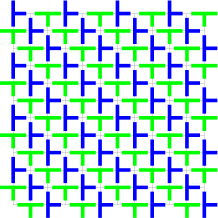
FIG. 10.: Two possible configurations of the Tetris model considered with the maximal density $\rho=\rho_{max}=2/3.$

B Equilibrium measure

The equilibrium measure is obtained with an annealing procedure. We can introduce a temperature $T=1/\beta$ associated with an energy $E$ defined as the total particle overlaps existing in a certain configuration. For each value of $T$ one allows the configurations with a probability given by $e^{-\beta E}$. Starting with a large temperature $T$ (a very small $\beta$) one samples the allowed configurations by progressively decreasing $T$ (increasing $\beta$). As $T$ is reduced $E$ decreases and only at $T=0$ (no violation of constraints allowed) the energy is precisely zero. The exploration of the configuration space can be performed in two ways:

• working at constant density by interchanging the positions of couples of particles. This procedure is used to compute $E(\beta,\rho)$ and $e(\beta,\rho)$ (energy per particle), from which one can compute the equilibrium entropy per particle by the expression:

  $$s_{equil}(\rho) \equiv s_{equil}(\beta=\infty,\rho)=$$ (20)

  $$= s_{equil}(\beta=0,\rho)-\int_{0}^{\infty}e(\beta,\rho)d\beta\,$$ (21)

  For the choice made for the particles one has

  $$s_{equil}(\beta=0,\rho) = -\rho\ln\rho-(1-\rho)\ln(1-\rho)$$ (23)

  $$+\rho\ln 4,$$

  which is easily obtained by counting the number of ways in which one can arrange $\rho L^{2}$ particles of four different types on $N=L^{2}$ sites;

• working at constant chemical potential $\mu$ by adding and removing particles. In this case the density fluctuates and one measures $E(\beta,\mu)$.

In both cases one can measure the particle-particle correlation function (equivalent to the void-void correlation function) $g_{equil}(r)$. Since, working at constant $\mu$ the density fluctuates, we have always measured directly the ensemble average $<(g_{equil}(r)-\rho^{2})>$ in order to make the data obtained with the two different methods comparable. One can then compare the correlation function obtained at constant $\mu$ (which corresponds to a certain average density) with the correlation function obtained working at constant density. The results of both methods are equivalent.

Fig.s (11) and (12) report the results for $e(\beta,\rho)$ and $s_{equil}(\rho)$ as obtained from (21).

FIG. 11.: $e(\beta=1/T,\rho)$ for various values of $\rho$. From top to bottom the density decreases monotonically from $\rho=0.6$ to $\rho=0.1$

FIG. 12.: Entropy per particle in equilibrium $s_{equil}(\rho)$ and, for reference, entropy per particle at $T_{aux}=\infty$. $s_{equil}(\rho)$ goes to zero at $\rho=\frac{2}{3}$.

Fig. 13 reports the results for $<(g_{equil}(r)-\rho^{2})>$ for different values of $\rho$. The correlation functions $g$ ($g_{equil}$ or $g_{edw}$ or $g_{dyn}$) actually display oscillations around $\rho^{2}$, whose origin can be easily understood: if a particle occupies a site, the exclusion rules decreases the probability that a neighboring site will be occupied. We therefore plot in the figures $<(g(r)-\rho^{2})>^{2}$ in order to show the exponential decay of the correlations.

FIG. 13.: $<(g_{equil}(r)-\rho^{2})>^{2}$ for various values of $\rho$. From top to bottom the density decreases monotonically from $\rho=0.64$ to $\rho=0.1$.

C Edwards’ measure

Edwards’ measure is obtained with an annealing procedure at fixed density. This means that one samples the configurational space by interchanging the positions of couples of particles without violations of constraints. In this way one is sampling the configurational space corresponding already to $T=0$. In order to select only the subset of configurations contributing to the Edwards’ measure we introduce an auxiliary temperature $T_{aux}$ (and the corresponding $\beta_{aux}=1/T_{aux}$) and, associated to it, an auxiliary energy $E_{aux}$ which, for each configuration, is equal to the number of mobile particles, in the same way as for the KA model. A particle is defined as mobile if it can be moved according to the dynamic rules of the original model.

Let us describe in detail how the measurements are performed. Since for each given density one is interested in the subset of the equilibrium configurations with a reduced particle mobility, we start with an annealing procedure precisely identical to the one used for the equilibrium measure. This procedure allows us to reach a starting configuration with a given density and no constraints violated. At this stage we perform a Monte Carlo procedure which exchanges the positions of couples of particles without violation of constraints: this procedure accepts the non-local moves with a standard Metropolis probability $\min(1,\exp(-\beta_{aux}\Delta E_{aux})$) which allow for an efficient sampling. These non-local moves define an auxiliary dynamics which has nothing to do with the true dynamics of the original model, and therefore the auxiliary model is not glassy.

As for the equilibrium we have performed a certain set of measures.

In particular we have measured $E_{aux}(\beta_{aux},\rho)$, i.e. the decrease of the auxiliary energy at fixed density. In order to do this one performs an annealing procedure increasing progressively $\beta_{aux}$ and monitoring for each $\beta_{aux}$ the corresponding configurational energy $E_{aux}(\beta_{aux},\rho)$. From this measure one can compute the Edwards’ entropy per particle defined by:

$$s_{edw}(\rho) \equiv s_{aux}(\beta_{aux}=\infty,\rho)=$$ (24)

$$= s_{equil}(\rho)-\int_{0}^{\infty}e_{aux}(\beta_{aux},\rho)d\beta_{aux}\,$$ (25)

where $e_{aux}(\beta_{aux},\rho)$ is the auxiliary Edwards’ energy per particle and we put $s_{equil}(\rho)=s_{aux}(\beta_{aux}=0,\rho)$.

Fig. 14 reports the results for $s_{edw}(\rho)$ as obtained from (25) compared with $s_{equil}(\rho)$.

FIG. 14.: Edwards’ entropy per particle, $s_{edw}(\rho)$ and equilibrium entropy per particle, $s_{equil}(\rho)$. Both go to zero at $\rho=\frac{2}{3}$.

For the computation of the particle-particle correlation function we have to use a different strategy. Always starting from a configuration with a given density and no constraints violated one performs a Monte Carlo procedure, at $\beta_{aux}$ fixed, which exchanges the positions of pairs of particles without violation of constraints. Each single simulation uses $\rho$ and $\beta_{aux}$ as input parameters. In practice one is trying to sample all the configuration of density $\rho$ and with a particle mobility defined by $\beta_{aux}$. In this context the Edwards’ prescription should correspond to the limit $\beta_{aux}\rightarrow\infty$. In this way we have computed $<(g_{edw}(r)-\rho^{2})>$ for several values of $\beta_{aux}$ and we report the results in Fig. 15. As one can see the limit $\beta_{aux}\rightarrow\infty$ is attained already for $\beta_{aux}$ of the order of $6$.

FIG. 15.: $<(g_{edw}(r)-\rho^{2})>^{2}$ for $\rho=0.58$; $\beta_{aux}=1,2,4,6$. The behaviour seems to saturate to a limit that should correspond to $\beta_{aux}\rightarrow\infty$ already for $\beta_{aux}$ of the order of $6$.

D Irreversible Compaction Dynamics

We now turn to the out of equilibrium dynamics of compaction, simulated by starting from an empty lattice and performing $N$ steps of attempted particle additions followed by $M$ steps of attempted particle diffusions. Fig. 16 reports the results for the density increase and for the fraction of mobiles particles as a function of the density for $N=1,M=1$ and $N=10,M=1$. While the limit $N=$ fixed $M->\infty$ should coincide with the equilibrium, it is clear that the system, at finite $M$, is not able to approach its maximum density and falls out of equilibrium. Here again the density at which the number of blocked configurations is maximal is smaller than the one achieved by compaction.

FIG. 16.: $\rho_{mob}$ vs. $\rho$ for two irreversible dynamics with $N=1,M=1$ and $N=10,M=1$. For reference is plotted the equilibrium curve.

It is particularly interesting to notice that in the out-of-equilibrium configurations visited during the irreversible dynamics the fraction of mobile particles $\rho_{mob}$ at fixed density is systematically smaller than the corresponding value in equilibrium. This suggests the possibility of distinguishing between equilibrium and out-of-equilibrium configurations by looking at the spatial organization of the particles in both cases. We have then measured, during the compaction dynamics, the particle-particle correlation function at fixed density. In the next section we shall compare these results with those obtained on the basis of the equilibrium and Edwards’ measures.

E Comparing different measures

We are now able, as for the KA model, to compare Gibbs’ and Edwards’ measures with the results of the out-of–equilibrium dynamics at large times.

In Fig. 17 we plot the deviations of the particle-particle correlation functions from the uncorrelated value $\rho^{2}$. In particular we compare $<(g_{dyn}(r)-\rho^{2})>^{2}$ obtained during the irreversible compaction ($N=1,M=1$) with the corresponding functions obtained with the equilibrium and Edwards’ measures. It is evident that the correlation function, as measured during the irreversible compaction dynamics, is significantly different from the one obtained with the equilibrium measure. On the other hand the correlation functions obtained with Edwards’ measure are able to better describe what happens during the irreversible dynamics. In particular what is observed is that the correlation length seems to be smaller for configurations explored by the irreversible dynamics than in the equilibrium configurations. This aspect is captured by Edwards’ measure which selects, the better the larger $\beta_{aux}$, configurations with a reduced particle mobility. In practice one can summarize the problem as follows: given a certain density, one can arrange the particles in different ways. The different configurations obtained in this way differ in the particle mobility and this feature is reflected by the change in the particle-particle correlation properties.

FIG. 17.: Comparison between the correlation functions obtained with the equilibrium measure, the Edwards measure ($\beta_{aux}=6$) and the irreversible dynamics ($N=1,M=1$). In all cases the system is considered at a density of $\rho\simeq 0.58$.

Also in this case, as in the KA example, it turns out that Edwards’ measure, constructed by a flat sampling of the blocked configurations, is able to reproduce the physical quantities measured at large times. Investigations are currently running to check also in the Tetris model whether the temperature predicted with the Edwards’ approach coincide with the dynamical temperature $T_{dyn}$ as defined for the KA model.

IV The 3-dimensional Random Field Ising Model at low temperature

In this section, we consider a case in which Edwards’ ensemble does not give good results: the low temperature domain growth dynamics of a 3D Ising model in a weak random magnetic field. This model has been applied in many different contexts [15], and in particular in relation with glasses [40]. The logarithmic relaxations it displays at low temperature, as well as the dependence on its thermal history (like the influence of the cooling rate) can also induce comparisons with granular compaction.

The model is defined as usual: $N=L^{3}$ Ising spins ($s_{i}=\pm 1$) sitting on the sites of a regular lattice of linear size $L$, interact ferromagnetically, in a random external field. The Hamiltonian is

$$H=-J\sum_{<i,j>}s_{i}s_{j}-\sum_{i}h_{i}s_{i}\ ,$$ (26)

where the sum runs over pairs of nearest neighbours.

The strength of the ferromagnetic interaction $J$ can be set to $1$, and the distribution of the random fields $h_{i}$ will be taken as bimodal $h_{i}=\pm h_{0}$. At high temperature, the system is in a paramagnetic phase; at low temperature and weak magnetic field, there exists a ferromagnetic phase (see [15]). The typical equilibrium configurations are therefore magnetized.

In the absence of random fields, the low temperature dynamics is the well known coarsening of domains of plus or minus spins, whose typical size grows as a power of time. In the case of the RFIM, the domain walls are pinned by the field, and the dynamics proceeds by thermal activation. The size of the domains therefore grows only logarithmically with time. Moreover, the fact that thermal barriers are easier to overcome at not too low temperatures induces a strong dependence on the cooling rate. As above, we are interested in the limit of low but non-zero temperatures.

In a large system, the long-time configurations obtained dynamically are intertwined domains of ‘up’ and ‘down’ spins having similar volumes, the global magnetization being zero. This is quite different from the equilibrium configurations at the same energy, which are magnetized. In fact, an easy way to show that the long-time dynamical configurations differ from the equilibrium ones is to look at the distribution of the magnetizations $P(M)$ in both cases: at equilibrium $P_{equil}(M)$ is peaked around $\pm M(T)$, with $M(T)>0$, while for the dynamics one obtains at any finite time for $P_{dyn}(M)$ a single peak around $M=0$: in this domain growth dynamics, the system does not choose at any finite time between the two basins of attractions of the two ground states [41].

The dynamics proceed by thermal activation; therefore the long-time configurations are ’blocked’, in the sense that, at zero temperature, the system would be unable to escape from them. The question in the present context is now whether these ’blocked configurations’ are typical, i.e. if their characteristics are well reproduced by a flat sampling of all blocked configurations of the same energy. We have therefore considered the corresponding auxiliary model, in order to obtain this flat sampling.

Since we want to study the configurations at a given energy, the auxiliary model has two terms: the first one is quadratic, constraining the energy (26) around a given $E_{0}$, and the second one is the number of spins not aligned with their local field, i.e. the number of spins that can flip without thermal activation:

$$E_{aux} = \beta_{1}\left(-J\sum_{<i,j>}s_{i}s_{j}-\sum_{i}h_{i}s_{i}-E_{0}\right)^{2}+$$ (28)

$$\beta_{2}\sum_{i}\Theta(-s_{i}{\cal H}_{i})\ \ ,$$

where $\Theta$ is the Heavyside function, and ${\cal H}_{i}=J\sum_{<j,i>}s_{j}+h_{i}$ is the local field at site $i$. The two auxiliary inverse temperatures $\beta_{1}$ and $\beta_{2}$ are used to perform an annealing, starting from a random initial configuration of high energy. We use a single-spin flip Metropolis algorithm, accepting the moves with probability $\min(1,\exp(-\Delta E_{aux}))$. $E_{0}$ is taken negative and slightly larger than the ground state mean energy $E_{GS}=-6JN$, in order to look at configurations having the same energy than the long time dynamics configurations (the evolution of the energy during the dynamical evolution is displayed in Fig. 18).

The first, simplest observable to look at is the distribution of the magnetization, $P_{edw}(M)$, averaged over realizations of disorder. Typical results are displayed in Fig. 19, for the $P(M)$ obtained dynamically or with a sampling of the blocked configurations, for a system of $20^{3}$ spins, and for $E_{0}=-5.4JN$ and $-5.2JN$ (we have also simulated systems of $30^{3}$ spins). While the dynamical $P_{dyn}(M)$ consists in a single peak around $M=0$ (getting narrower for larger system sizes), the distribution $P_{edw}(M)$ is clearly bimodal, presenting two peaks around two symmetric values of the magnetization. The precise values of the peaks depend on $E_{0}$ (decreasing for increasing $E_{0}$: it is clear that, for too high values of $E_{0}$, the configurations are less magnetized), and their width depend on system size, getting narrower for larger systems.

FIG. 18.: Energy versus time for the dynamics of the RFIM at inverse temperatures $3$, $4$ and $5$. The energy decreases slower for larger $\beta$ because the dynamics is activated. For one given sample $E(t)$ would be a succession of plateaus, here the curves correspond to an average over $64$ realizations of the random field.

It appears therefore that the configurations dominating Edwards’ distribution are magnetized. (Note that a similar result was obtained in [42] for the low-energy metastable states for a ferromagnet on random thin graphs). At variance with the previously studied models (KA and Tetris), Edwards’ distribution is therefore unable to describe the typical configurations obtained dynamically.

The example of the RFIM clearly underlines the difference with the inherent structure construction of Kob et al. On the one hand, we have seen that Edwards’ measure does not reproduce the dynamic results. On the other hand, it is clear that different thermal histories, just as those considered in [28], would yield domain configurations with essentially the same shapes if the end energy is the same, and zero magnetization, contrary to the typical configurations at that energy.

FIG. 19.: Histograms of the magnetization of the visited configurations during the low temperature dynamics (full line: $P_{dyn}(M)$ for $L=20$, $\beta=4$, i.e. the energy per site of the system is between $-5.2$ and $-5.4$; the finite width of the peak comes from the relatively small size of the sample) and for Edwards’ measure at $E_{0}=-5.2$ and $-5.4$ (dotted, dashed, long-dashed and dot-dashed lines: $P_{edw}(M)$ for $L=20$ and $\beta_{2}=4$ and $6$; $E_{0}=-5.4$ corresponds to the peaks at higher $M$). The dynamics samples configurations with low magnetization, while the typical blocked configurations are magnetized.

V ‘Chaoticity’ properties

We have shown two models for which Edwards’ construction gives a good approximation, and one for which it does not. What is the distinguishing feature between them? A distinction one can make, suggested by glass theory [43, 44, 45, 24], is obtained by studying their ‘chaoticity’ properties as follows: after aging for a time $t_{w}$, two copies (clones) are made of the system, and allowed to evolve subsequently with different realizations of the randomness in the updating procedure. The question is then whether the trajectories diverge or not. Note that for this criterion to make sense, it should always be applied at non-zero (though weak) tapping or shearing.

The results summarized below seem to indicate that the condition of chaoticity is necessary. It is however not sufficient: Bouchaud’s ‘trap model’ [19] is chaotic but its fluctuation-dissipation properties are not directly related to the density of states [46].

For the three models discussed in this paper, we have measured the normalized average overlap $Q_{t_{w}}(t)$ defined as

• for the KA model

  $$Q_{t_{w}}(t)=\langle\frac{1}{N}\sum_{i}n_{i}(t)n_{i}^{clone}(t)-\rho(t)\cdot\rho_{clone}(t)\rangle$$ (29)

  where $n_{i}$ (resp. $n_{i}^{clone}$) is $1$ if there is a particle on the site $i$ for the original model (resp. for the clone), and $0$ if the site is empty;

• for the Tetris model

  $$Q_{t_{w}}(t)=\langle\frac{(\frac{1}{N}\sum_{i,j}A_{i,j}(t)-\frac{\rho(t)\cdot\rho_{clone}(t)}{4})}{(\rho_{clone}(t)-\frac{\rho_{clone}(t)^{2}}{4})}\rangle$$ (30)

  where $A_{i,j}(t)$ is a function that gives one if on the site $(i,j)$ the two copies present the same particles and zero otherwise. We have four types of particles in the system and this is the reason for the factors $4$ in (30).

• for the RFIM

  $$Q_{t_{w}}(t)=\langle\frac{1}{N}\sum_{i}s_{i}(t)s_{i}^{clone}(t)\rangle$$ (31)

The brackets indicate an average over different realizations of the randomness.

Fig. 20 and 21 report the results for $Q_{t_{w}}(t)$ for several values of $t_{w}$, respectively for the Tetris and the KA model. It is clear that in both cases the two copies of the system always tend to diverge. This is at variance with what happens in the domain growth dynamics [45], and in particular for the RFIM, where we have checked that the two copies retain a finite overlap at all the times studied.

FIG. 20.: Mean overlap $Q_{t_{w}}(t)$ between two clones in the Tetris model: the two clones are separated at $t_{w}$ and evolve subsequently with different noises. $Q_{t_{w}}(t)$ always decreases to zero (the slower the larger $t_{w}$), showing that the clones always diverge.

FIG. 21.: Same as Fig. 20 for the KA model.

VI Conclusions

In summary, we have proposed a simple and systematic procedure to construct a flat sampling of the ‘blocked configurations’, i.e. to calculate averages with Edwards’ measure. We have shown, for two representative finite-dimensional models, that this measure gives different results than the equilibrium measure, and is able to reproduce the dynamical sampling of the out-of-equilibrium compaction dynamics for various observables. The connection of Edwards’ ensemble with the dynamical FDT temperature immediately suggests experiments to check the validity of these ideas, for example by studying diffusion and mobility of different tracer particles within driven granular media.

At present, the correspondence between Edwards’ distribution and the long-time dynamics is at best checked but does not follow from any known principle. Now that several concrete examples have lent credibility to Edwards’ construction, an effort to understand why it does in some cases work and what is its range of validity has become worthwhile.

There remains the question of generalizing Edwards’ measures in two directions: by considering a fraction $\epsilon>0$ of mobile particles, and by conditioning the flat measure to more macroscopic observables in addition to density and energy.

V.L. and M.S. acknowledge the hospitality of the ESPCI of Paris where part of this work was carried out. MS is supported by a Marie Curie fellowship of the European Commission (contract ERBFMBICT983561). This work has also been partially supported from the European Network-Fractals under contract No. FMRXCT980183.

REFERENCES

- [1]
- [2]
- [3] Unité Mixte de Recherche UMR 8627.
- [4]
- [5] H.M. Jaeger, S.R. Nagel, Science 255, 1523 (1992).
- [6] H.M. Jaeger, S.R. Nagel, and R.P. Behringer, Rev. Mod. Phys 68, 1259 (1996).
- [7] J. B. Knight, C. G. Fandrich, C. N. Lau, H. M. Jaeger, and S. R. Nagel, Phys. Rev. E 51, 3957 (1995).
- [8] S.F. Edwards, in: Granular Matter: An Interdisciplinary Approach, A. Mehta, Ed. (Springer-Verlag, New York, 1994), and references therein.
- [9] A. Mehta, R.J. Needs, S. Dattagupta, J. Stat. Phys. 68, 1131 (1992).
- [10] R. Monasson, O. Pouliquen, Physica A 236, 395 (1997).
- [11] A. Barrat, J. Kurchan, V. Loreto and M. Sellitto, Phys. Rev. Lett. 85 5034 (2000).
- [12] See, for example Chapter 7 of: L.C.E. Struik, Physical Ageing in Amorphous Polymers and Other materials, (Elsevier, Houston, 1978).
- [13] W. Kob, H.C. Andersen, Phys. Rev. E 48, 4364 (1993).
- [14] E. Caglioti, V. Loreto, H.J. Herrmann and M. Nicodemi, Phys. Rev. Lett. 79, 1575 (1997).
- [15] T. Nattermann, in Spin-glasses and random fields, A. P. Young, Ed. (World Scientific, Singapore, 1997).
- [16] E. Ott, Chaos in Dynamical Systems (Cambridge University Press, Cambridge 1993).
- [17] T.R. Kirkpatrick, D. Thirumalai, Phys. Rev. B 36, 5388 (1987).
- [18] T.R. Kirkpatrick, P. Wolynes, Phys. Rev. A 35, 3072 (1987).
- [19] J.-P. Bouchaud, L.F. Cugliandolo, J. Kurchan and M. Mézard, in Spin-glasses and random fields, A. P. Young, Ed. (World Scientific, Singapore, 1997).
- [20] L.F. Cugliandolo, J. Kurchan, L. Peliti, Phys. Rev. E 55, 3898 (1997).
- [21] R. Monasson, Phys. Rev. Lett. 75, 2847 (1995).
- [22] J. Kurchan, in Jamming and Rheology: Constrained Dynamics on Microscopic and Macroscopic Scales (1997), http://www.itp.ucsb.edu/online/jamming2/, and Edwards, S.F., Liu, A. and Nagel, S.R. Eds., to be published, cond-mat 9812347.
- [23] Th.M. Nieuwenhuizen, Phys. Rev. E 61, 267 (2000).
- [24] S. Franz, M.A. Virasoro, J. Phys. A 33, 891 (2000).
- [25] A. Crisanti, F. Ritort, cond-mat/9911226.
- [26] G. Biroli and J. Kurchan, Phys. Rev. E, to be published.
- [27] J. Kurchan, J. Phys. Condensed Matter, 12, 6611 (2000).
- [28] W. Kob, F. Sciortino, P. Tartaglia, Europhys. Lett. 49, 590 (2000).
- [29] P. H. Stillinger and T. A. Weber, Phys. Rev. A25, 978 (1982); S. Sastry, P. G. Debenedetti and F. H. Stillinger, Nature 393, 554 (1998); B. Coluzzi, G. Parisi and P. Verrocchio, Phys. Rev. Lett.84, 306 (2000); F. Sciortino, W. Kob, and P. Tartaglia, Phys. Rev. Lett.83 3214 (1999).
- [30] A. Coniglio and M. Nicodemi, cond-mat/0010191.
- [31] For a review, see: W. Götze, in ‘Liquids, freezing and glass transition’, J.P. Hansen, D. Levesque, J. Zinn-Justin Editors, Les Houches (1989) (North Holland).
- [32] J. Kurchan, L. Peliti, M. Sellitto, Europhys. Lett. 39, 365 (1997).
- [33] M. Sellitto, Euro. J. Phys. B 4, 135 (1998).
- [34] M. Sellitto, J.J. Arenzon, Free-volume kinetic models of granular matter, Phys. Rev. E (December 2000).
- [35] A. Barrat, V. Loreto, J. Phys. A. 33, 4401 (2000)
- [36] E. Caglioti, A. Coniglio, H.J. Herrmann, V. Loreto and M. Nicodemi, Europhys. Lett. 43, 591 (1998).
- [37] M. Piccioni, V. Loreto and S. Roux, Phys. Rev. E 61, 2813 (1999).
- [38] A. Barrat, V. Loreto, Europhys. Lett. (2000).
- [39] M. Nicodemi, A. Coniglio, Phys. Rev. Lett. 82, 916 (1999).
- [40] See e.g. F. Alberici-Kious, J.P. Bouchaud, L. Cugliandolo, P. Doussineau and A. Levelut, Phys. Rev. Lett. 81, 4987 (1998).
- [41] J. Kurchan and L. Laloux, J. Phys. A 29 (1996) 1929.
- [42] A. Lefevre, D. S. Dean, Metastable states of a ferromagnet on random thin graphs, cond-mat/0011265.
- [43] A. Baldassarri, Laurea Thesis, University of Rome La Sapienza, (1995).
- [44] L.F. Cugliandolo, D.S. Dean, J. Phys. A 28, 4213 (1995).
- [45] A. Barrat, R. Burioni, M. Mézard, J. Phys. A 29, 1311 (1996).
- [46] J-P. Bouchaud: private communication.