High-Order Coupled Cluster Method Calculations for the Ground- and Excited-State Properties of the Spin-Half XXZ Model

Abstract

In this article, we present new results of high-order coupled cluster method (CCM) calculations, based on a Néel model state with spins aligned in the $z$-direction, for both the ground- and excited-state properties of the spin-half XXZ model on the linear chain, the square lattice, and the simple cubic lattice. In particular, the high-order CCM formalism is extended to treat the excited states of lattice quantum spin systems for the first time. Completely new results for the excitation energy gap of the spin-half XXZ model for these lattices are thus determined. These high-order calculations are based on a localised approximation scheme called the LSUB$m$ scheme in which we retain all $k$-body correlations defined on all possible locales of $m$ adjacent lattice sites ($k\leq m$). The “raw” CCM LSUB$m$ results are seen to provide very good results for the ground-state energy, sublattice magnetisation, and the value of the lowest-lying excitation energy for each of these systems. However, in order to obtain even better results, two types of extrapolation scheme of the LSUB$m$ results to the limit $m\rightarrow\infty$ (i.e., the exact solution in the thermodynamic limit) are presented. The extrapolated results provide extremely accurate results for the ground- and excited-state properties of these systems across a wide range of values of the anisotropy parameter.

PACS numbers: 75.10.Jm, 75.50Ee, 03.65.Ca

I Introduction

The coupled cluster method (CCM) newccm1 ; newccm2 ; newccm3 ; newccm4 ; newccm5 ; newccm6 ; newccm7 ; newccm8 has previously been applied ccm1 ; ccm2 ; ccm3 ; ccm4 ; ccm5 ; ccm6 ; ccm7 ; ccm8 ; ccm9 ; ccm10 ; ccm11 ; ccm12 ; ccm13 ; ccm14 to various lattice quantum spin systems with much success. In particular, high-order ccm7 ; ccm8 ; ccm9 ; ccm11 ; ccm12 ; ccm13 CCM calculations using a localised approximation scheme called the LSUB$m$ approximation scheme have previously been utilised to determine the ground-state properties of the spin-half square lattice XXZ model to high accuracy (see especially Refs. ccm7 ; ccm11 ). These calculations were performed both in a regime characterised by non-zero Néel order ccm1 ; ccm2 ; ccm3 ; ccm7 in the $z$-direction, and also in a regime characterised by non-zero Néel ordering in the $xy$-plane ccm8 ; ccm11 . The results were found to be in excellent agreement with the known results of the XXZ model (discussed below).

The spin-half XXZ model is defined by the following Hamiltonian,

$$H=\frac{1}{2}\sum_{i=1}^{N}\sum_{\rho}\left[s_{i}^{x}s_{i+\rho}^{x}+s_{i}^{y}s_{i+\rho}^{y}+\Delta s_{i}^{z}s_{i+\rho}^{z}\right]~{}~{},$$ (1)

where the index i in Eq. (1) runs over all $N$ lattice sites, and $\rho$ runs over all z nearest-neighbours lattice vectors with respect to $i$ on the chain (z=2), the square lattice (z=4), and the simple cubic lattice (z=6). Periodic boundary conditions are also assumed. We note that $[H,s_{T}^{z}]=0$ for this model, where $s_{T}^{z}=\sum_{i=1}^{N}s_{i}^{z}$. The spin-half XXZ model contains three regimes with respect to the anisotropy parameter $\Delta$. For $\Delta\leq-1$ there is a ferromagnetic regime in which the classical ground state is also the quantum-mechanical ground state. At $\Delta=-1$, there is a first-order phase transition to a planar regime in which the classical ground state is a Néel state in the $xy$-plane. For the square and cubic lattices, the quantum-mechanical ground state in this regime is furthermore characterised by non-zero, in-plane, long-range ordering. For the linear chain quantum fluctuations are strong enough to destroy all long-range ordering and so this region in 1D is sometimes referred to as the “critical regime.” In the 1D case the planar regime spans the range $-1<\Delta<1$, and at $\Delta=1$ there is another phase transition to a phase characterised by non-zero Néel ordering in the $z$-direction for the ground state. For the linear chain, the Bethe Ansatz ba1 ; ba2 ; ba3 ; ba4 provides an exact solution of the quantum spin-half XXZ model, although for higher spatial dimensionality no exact solutions have as yet been determined. However, extensive approximate calculations have been carried out for this model, in particular for the Heisenberg antiferromagnet (HAF) at $\Delta=1$. It is believed that the 1D phase transition at $\Delta=1$ also occurs for higher spatial dimensionality than one. Examples of such approximate calculations for the spin-half XXZ and HAF models are spin-wave theory swt1 ; swt2 (SWT), exact diagonalisations of finite-sized systems finite1 ; finite2 , exact cumulant series expansions series1 , and quantum Monte Carlo qmc1 ; qmc2 ; qmc3 ; qmc4 (QMC) calculations. In particular, we note that such results for the spin-half isotropic HAF on the square lattice typically predict that approximately 61-62$\%$ of the classical Néel-ordering remains in the quantum case.

In this article we present results of high-order coupled CCM calculations for the ground- and excited-state properties of the spin-half XXZ model on the linear chain, square lattice, and simple cubic lattice based on the systematic incorporation of many-spin correlations on top of a Néel model state with spins aligned in the $z$-direction. In Sec. II, we describe the high-order CCM formalisms for both the ground and excited states. Although the high-order CCM formalism has been described previously ccm11 , we present a very brief overview of it in order to give a necessary background for the new high-order formalism for the excited state. We also discuss in Sec. II the manner in which the CCM results for a localised approximation scheme called the LSUB$m$ scheme (in which we retain all $k$-body correlations defined on all possible locales of $m$ adjacent lattice sites ($k\leq m$)) are extrapolated to the limit $m\rightarrow\infty$. In Sec. III, we present the results of our high-order treatment of the XXZ model for these lattices, and finally our conclusions are presented in Sec. IV.

II The Coupled Cluster Method (CCM)

In this section, we firstly describe the general ground-state CCM formalism newccm1 ; newccm2 ; newccm3 ; newccm4 ; newccm5 ; newccm6 ; newccm7 ; newccm8 , and then show how to apply it to the specific case of the spin-half XXZ model. This is then extended to deal with excited states.

II.1 The Ground-State Formalism

The exact ket and bra ground-state energy eigenvectors, $|\Psi\rangle$ and $\langle\tilde{\Psi}|$, of a many-body system described by a Hamiltonian $H$,

$$H|\Psi\rangle=E_{g}|\Psi\rangle\;;\;\;\;\langle\tilde{\Psi}|H=E_{g}\langle\tilde{\Psi}|\;,$$ (2)

are parametrised within the single-reference CCM as follows:

$$|\Psi\rangle={\rm e}^{S}|\Phi\rangle\; \;\;\;S=\sum_{I\neq 0}{\cal S}_{I}C_{I}^{+}\;,$$ ;

$$\langle\tilde{\Psi}|=\langle\Phi|\tilde{S}{\rm e}^{-S}\; \;\;\;\tilde{S}=1+\sum_{I\neq 0}\tilde{{\cal S}}_{I}C_{I}^{-}\;.$$ ; (3)

The single model or reference state $|\Phi\rangle$ is required to have the property of being a cyclic vector with respect to two well-defined Abelian subalgebras of multi-configurational creation operators $\{C_{I}^{+}\}$ and their Hermitian-adjoint destruction counterparts $\{C_{I}^{-}\equiv(C_{I}^{+})^{\dagger}\}$. Thus, $|\Phi\rangle$ plays the role of a vacuum state with respect to a suitable set of (mutually commuting) many-body creation operators $\{C_{I}^{+}\}$,

$$C_{I}^{-}|\Phi\rangle=0\;\;,\;\;\;I\neq 0\;,$$ (4)

with $C_{0}^{-}\equiv 1$, the identity operator. These operators are complete in the many-body Hilbert (or Fock) space,

$$1=|\Phi\rangle\langle\Phi|+\sum_{I\neq 0}C_{I}^{+}|\Phi\rangle\langle\Phi|C_{I}^{-}\;.$$ (5)

The correlation operator $S$ is decomposed entirely in terms of these creation operators $\{C_{I}^{+}\}$, which, when acting on the model state ($\{C_{I}^{+}|\Phi\rangle\}$), create multi-particle excitations on top of the model state. We note that although the manifest Hermiticity, ($\langle\tilde{\Psi}|^{\dagger}=|\Psi\rangle/\langle\Psi|\Psi\rangle$), is lost in these parametrisations, the intermediate normalisation condition $\langle\tilde{\Psi}|\Psi\rangle=\langle\Phi|\Psi\rangle=\langle\Phi|\Phi\rangle\equiv 1$ is explicitly imposed. The correlation coefficients $\{{\cal S}_{I},\tilde{{\cal S}}_{I}\}$ are regarded as being independent variables, even though formally we have the relation,

$$\langle\Phi|\tilde{S}=\frac{\langle\Phi|{\rm e}^{S^{\dagger}}{\rm e}^{S}}{\langle\Phi|{\rm e}^{S^{\dagger}}{\rm e}^{S}|\Phi\rangle}\;.$$ (6)

The full set $\{{\cal S}_{I},\tilde{{\cal S}}_{I}\}$ thus provides a complete description of the ground state. For instance, an arbitrary operator $A$ will have a ground-state expectation value given as,

$$\bar{A}\equiv\langle\tilde{\Psi}|A|\Psi\rangle=\langle\Phi|\tilde{S}{\rm e}^{-S}A{\rm e}^{S}|\Phi\rangle=\bar{A}\left(\{{\cal S}_{I},\tilde{{\cal S}}_{I}\}\right)\;.$$ (7)

We note that the exponentiated form of the ground-state CCM parametrisation of Eq. (3) ensures the correct counting of the independent and excited correlated many-body clusters with respect to $|\Phi\rangle$ which are present in the exact ground state $|\Psi\rangle$. It also ensures the exact incorporation of the Goldstone linked-cluster theorem, which itself guarantees the size-extensivity of all relevant extensive physical quantities.

The determination of the correlation coefficients $\{{\cal S}_{I},\tilde{{\cal S}}_{I}\}$ is achieved by taking appropriate projections onto the ground-state Schrödinger equations of Eq. (2). Equivalently, they may be determined variationally by requiring the ground-state energy expectation functional $\bar{H}(\{{\cal S}_{I},\tilde{{\cal S}}_{I}\})$, defined as in Eq. (7), to be stationary with respect to variations in each of the (independent) variables of the full set. We thereby easily derive the following coupled set of equations,

$$\delta{\bar{H}}/\delta{\tilde{{\cal S}}_{I}}=0 \Rightarrow \langle\Phi|C_{I}^{-}{\rm e}^{-S}H{\rm e}^{S}|\Phi\rangle=0,\;\;\forall I\neq 0\;\;;$$ (8)

$$\delta{\bar{H}}/\delta{{\cal S}_{I}}=0 \Rightarrow \langle\Phi|\tilde{S}{\rm e}^{-S}[H,C_{I}^{+}]{\rm e}^{S}|\Phi\rangle=0,\;\;\forall I\neq 0\;\;.$$ (9)

Equation (8) also shows that the ground-state energy at the stationary point has the simple form

$$E_{g}=E_{g}(\{{\cal S}_{I}\})=\langle\Phi|{\rm e}^{-S}H{\rm e}^{S}|\Phi\rangle\;\;.$$ (10)

It is important to realize that this (bi-)variational formulation does not lead to an upper bound for $E_{g}$ when the summations for $S$ and $\tilde{S}$ in Eq. (3) are truncated, due to the lack of exact Hermiticity when such approximations are made. However, it is clear that the important Hellmann-Feynman theorem is preserved in all such approximations.

We also note that Eq. (8) represents a coupled set of nonlinear multinomial equations for the c-number correlation coefficients $\{{\cal S}_{I}\}$. The nested commutator expansion of the similarity-transformed Hamiltonian,

$$\hat{H}\equiv{\rm e}^{-S}H{\rm e}^{S}=H+[H,S]+{1\over 2!}[[H,S],S]+\cdots\;\;,$$ (11)

together with the fact that all of the individual components of $S$ in the sum in Eq. (3) commute with one another, imply that each element of $S$ in Eq. (3) is linked directly to the Hamiltonian in each of the terms in Eq. (11). Thus, each of the coupled equations (8) is of linked-cluster type. Furthermore, each of these equations is of finite length when expanded, since the otherwise infinite series of Eq. (11) will always terminate at a finite order, provided (as is usually the case) only that each term in the second-quantised form of the Hamiltonian $H$ contains a finite number of single-body destruction operators, defined with respect to the reference (vacuum) state $|\Phi\rangle$. Therefore, the CCM parametrisation naturally leads to a workable scheme which can be efficiently implemented computationally. It is also important to note that at the heart of the CCM lies a similarity transformation, in contrast with the unitary transformation in a standard variational formulation in which the bra state $\langle\tilde{\Psi}|$ is simply taken as the explicit Hermitian adjoint of $|\Psi\rangle$.

We now wish to apply the general CCM formalism outlined above to the specific case of the spin-half XXZ model, and we choose the Néel state, in which the spins lie along the $z$-axis, to be the model state. Furthermore, we perform a rotation of the local axes of the up-pointing spins by 180^∘ about the $y$ axis, so that spins on both sublattices may be treated equivalently. The (canonical) transformation is described by,

$$s^{x}\;\rightarrow\;-s^{x},\;s^{y}\;\rightarrow\;s^{y},\;s^{z}\;\rightarrow\;-s^{z}\;.$$ (12)

The model state now appears $mathematically$ to consist of purely down-pointing spins in these rotated local axes. In terms of the spin raising and lowering operators $s_{k}^{\pm}\equiv s_{k}^{x}\pm is_{k}^{y}$ the Hamiltonian may be written in these local axes as,

$$H=-\frac{1}{4}\sum_{i}^{N}\sum_{\rho}\;\biggl{[}\;s_{i}^{+}s_{i+\rho}^{+}+s_{i}^{-}s_{i+\rho}^{-}+2\Delta s_{i}^{z}s_{i+\rho}^{z}\;\biggr{]}\;.$$ (13)

In this article, we also wish to perform high-order CCM calculations for this model, and in order to do this we firstly define the $\{C_{I}^{+}\}$ operators more explicitly, as $C_{I}^{+}\equiv s^{+}_{i_{1}}s^{+}_{i_{2}}\cdot\cdot\cdot s^{+}_{i_{l}}$, where the set-index $I\equiv\{i_{1},i_{2},...,i_{l}\}$. Each of the single-site indices is allowed to cover all lattice sites, although double (or greater) occupancy of any particular site in any set $I$ is explicitly prohibited for the spin-half case, since $(s^{+})^{2}=0$. We analogously define the ket-state correlation coefficients as ${\cal S}_{I}\equiv{\cal S}_{i_{1},i_{2},\cdot\cdot\cdot,i_{l}}$ for a cluster $I$ defined above. By construction the coefficients ${\cal S}_{i_{1},i_{2},\cdot\cdot\cdot,i_{l}}$ are completely symmetric under the interchange of any two indices. It is also useful to define the following two operators,

$$F_{k} \equiv \sum_{l}\sum_{{i_{1}\cdot\cdot\cdot i_{l-1}}}l~{}{\cal S}_{k,i_{1},\cdot\cdot\cdot,i_{l-1}}~{}s^{+}_{i_{1}}\cdot\cdot\cdot s^{+}_{i_{l-1}}~{}~{};$$ (14)

$$G_{km} \equiv \sum_{l}\sum_{{i_{1}\cdot\cdot\cdot i_{l-2}}}l(l-1)~{}{\cal S}_{k,m,i_{1},\cdot\cdot\cdot,i_{l-2}}~{}s^{+}_{i_{1}}\cdot\cdot\cdot s^{+}_{i_{l-2}}~{}~{}.$$ (15)

The similarity transform of the Hamiltonian of Eq. (7) may now be written in terms of these operators. We find explicitly that $\hat{H}|\Phi\rangle\equiv e^{-S}He^{S}|\Phi\rangle=(\hat{H}_{1}+\hat{H}_{2}+\hat{H}_{3})|\Phi\rangle$, where

$$\hat{H}_{1} \equiv -\frac{1}{2}\sum_{i}\sum_{\rho}\biggl{\{}\Delta(G_{i,{i+\rho}}+F_{i}F_{i+\rho})+\frac{1}{2}+G^{2}_{i,{i+\rho}}$$ (16)

$$~{}~{}~{}~{}~{}~{}~{}~{}~{}~{}~{}~{}~{}~{}~{}~{}+2G_{i,{i+\rho}}F_{i}F_{i+\rho}+\frac{1}{2}F^{2}_{i}F^{2}_{i+\rho}\biggr{\}}s_{i}^{+}s_{i+\rho}^{+}~{}~{},$$

$$\hat{H}_{2} \equiv \frac{1}{2}\sum_{i}\sum_{\rho}\biggl{\{}\frac{\Delta}{2}(F_{i+\rho}s_{i+\rho}^{+}+F_{i}s_{i}^{+})+(G_{i,{i+\rho}}+\frac{1}{2}F_{i}F_{i+\rho})(F_{i+\rho}s_{i+\rho}^{+}+F_{i}s_{i}^{+})\biggr{\}}~{}~{},$$ (17)

$$\hat{H}_{3} \equiv -\frac{1}{4}\sum_{i}\sum_{\rho}\biggl{\{}\frac{\Delta}{2}+G_{i,{i+\rho}}+F_{i}F_{i+\rho}\biggr{\}}~{}~{}.$$ (18)

We note that the similarity-transformed Hamiltonian acting on the model state $|\Phi\rangle$ has now been written purely in terms of spin-raising operators. The problem of determining a given CCM ket-state equation, defined by Eq. (8) for a given cluster of index $I$, thus becomes an exercise in pattern-matching the spin-lowering operators in $C_{I}^{-}$ to the terms in $\hat{H}$ contained in Eqs. (16-18). This task is perfectly suited to implementation using computer algebra techniques, and the ensuing set of coupled, non-linear ket-state equations is then easily solved (for example, using the Newton-Raphson method). Once the ket-state correlation coefficients have been determined it is then possible to find the bra-state coefficients similarly, as described in Ref. ccm11 . One may finally calculate any ground-state expectation values that one wishes to obtain in terms of the coefficients $\{{\cal S}_{I},\tilde{{\cal S}_{I}}\}$. An example of this is the sublattice magnetisation, given by

$$M=-\frac{2}{N}\langle\tilde{\Psi}\mid\sum_{i=1}^{N}s_{i}^{z}\mid\Psi\rangle~{}~{},$$ (19)

in the rotated spin coordinates defined above. The quantity provides a measure for the amount of Néel ordering in the $z$-direction remaining in the CCM ground state, $|\Psi\rangle$, with respect to the perfect ordering ($M=1$) of the model state.

The CCM formalism is exact in the limit of inclusion of all possible multi-spin cluster correlations within $S$ and $\tilde{S}$, although in any real application this is usually impossible to achieve. It is therefore necessary to utilise various approximation schemes within $S$ and $\tilde{S}$. The three most commonly employed schemes have been: (1) the SUB$n$ scheme, in which all correlations involving only $n$ or fewer spins are retained, but no further restriction is made concerning their spatial separation on the lattice; (2) the SUB$n$-$m$ sub-approximation, in which all SUB$n$ correlations spanning a range of no more than $m$ adjacent lattice sites are retained; and (3) the localised LSUB$m$ scheme, in which all multi-spin correlations over distinct locales on the lattice defined by $m$ or fewer contiguous sites are retained. Note that for this system we also make the specific and explicit restriction that the creation operators $\{C_{I}^{+}\}$ in $S$ preserve the relationship that, in the original (unrotated) spin coordinates, $s^{z}_{T}=\sum_{i}s^{z}_{i}=0$ in order to keep the approximate CCM ground-state wave function in the correct ($s^{z}_{T}=0$) subspace. The number of such distinct (or fundamental) configurations for the ground state at a given level of approximation is labelled by $N_{F}$. We denote as distinct configurations those which are inequivalent under the point and space group symmetries of the both the lattice and the Hamiltonian.

In practice we find that the CCM equations often terminate at specific critical values (denoted $\Delta_{c}$) of the anisotropy parameter which are dependent on the particular approximation scheme chosen, such that no solution based on this model state exists for $\Delta<\Delta_{c}$. At these critical points the second derivative of the ground-state energy is found to diverge, and the critical points have been shown to reflect the corresponding phase transition point in the real system.

II.2 The Excited-State Formalism

We now turn our attention to the CCM parametrisation of the excited state developed by Emrich ccm15 , and as a specific example we present results for the high-order treatment of the excited states of the spin-half XXZ model. An excited-state wave function, $|\Psi_{e}\rangle$, is determined by linearly applying an excitation operator $X^{e}$ to the ket-state wave function of Eq. (3), such that

$$|\Psi_{e}\rangle=X^{e}~{}e^{S}|\Phi\rangle~{}~{}.$$ (20)

This equation may now be used to determine the low-lying excitation energies, such that the Schrödinger equation, $E_{e}|\Psi_{e}\rangle=H|\Psi_{e}\rangle$, may be combined with its ground-state counterpart of Eq. (2) to give the result,

$$\epsilon_{e}X^{e}|\Phi\rangle=e^{-S}[H,X^{e}]e^{S}|\Phi\rangle~{}(\equiv\hat{R}|\Phi\rangle)~{}~{},$$ (21)

where $\epsilon_{e}\equiv E_{e}-E_{g}$ is the excitation energy. By analogy with the ground-state formalism, the excited-state correlation operator is written as,

$$X^{e}=\sum_{I\neq 0}{\cal X}_{I}^{e}C_{I}^{+}~{}~{},$$ (22)

where the set $\{C_{I}^{+}\}$ of multi-spin creation operators may differ from those used in the ground-state parametrisation in Eq. (3) if the excited state has different quantum numbers than the ground state. We note that Eq. (22) implies the overlap relation $\langle\Phi|\Psi_{e}\rangle=0$. By applying $\langle\Phi|C_{I}^{-}$ to Eq. (21) we find that,

$$\epsilon_{e}{\cal X}_{I}^{e}=\langle\Phi|C_{I}^{-}e^{-S}[H,X^{e}]e^{S}|\Phi\rangle~{}~{},\forall I\neq 0~{}~{},$$ (23)

which is a generalised set of eigenvalue equations with eigenvalues $\epsilon_{e}$ and corresponding eigenvectors ${\cal X}_{I}^{e}$, for each of the excited states which satisfy $\langle\Phi|\Psi_{e}\rangle=0$. Analogously to the ground-state case, we define the excited-state operators

$$P_{k} \equiv \sum_{l}\sum_{i_{1}\cdots i_{l-1}}l~{}{\cal X}_{k,i_{1},\cdot\cdot\cdot i_{l-1}}^{e}~{}s^{+}_{i_{1}}\cdot\cdot\cdot s^{+}_{i_{l-1}}~{}~{},$$ (24)

$$Q_{km} \equiv \sum_{l}\sum_{i_{1}\cdots i_{l-2}}l(l-1)~{}{\cal X}_{k,m,i_{1},\cdot\cdot\cdot,i_{l-2}}^{e}~{}s^{+}_{i_{1}}\cdot\cdot\cdot s^{+}_{i_{l-2}}~{}~{}.$$ (25)

The state, $\hat{R}|\Phi\rangle\equiv e^{-S}[H,X^{e}]e^{S}|\Phi\rangle$, may now be divided into three elements, $\hat{R}|\Phi\rangle=(\hat{R}_{1}+\hat{R}_{2}+\hat{R}_{3})|\Phi\rangle$, such that (after collecting together like terms) we find the following expressions,

$$\hat{R}_{1} \equiv -\sum_{i}\sum_{\rho}\biggl{\{}\Delta(P_{i}F_{i+\rho}+\frac{1}{2}Q_{i,{i+\rho}})+2P_{i}F_{i+\rho}G_{i,{i+\rho}}$$ (26)

$$~{}~{}~{}~{}~{}~{}~{}~{}~{}~{}~{}~{}+Q_{i,{i+\rho}}G_{i,{i+\rho}}+Q_{i,{i+\rho}}F_{i}F_{i+\rho}+P_{i}F_{i}F_{i+\rho}^{2}\biggr{\}}s_{i}^{+}s_{i+\rho}^{+}~{}~{},$$

$$\hat{R}_{2} \equiv \sum_{i}\sum_{\rho}\biggl{\{}\frac{\Delta}{2}P_{i}s_{i}^{+}+P_{i}G_{i,{i+\rho}}s_{i}^{+}+P_{i}F_{i}F_{i+\rho}s_{i}^{+}$$ (27)

$$~{}~{}~{}~{}~{}~{}~{}~{}~{}~{}+\frac{1}{2}P_{i}F_{i+\rho}F_{i+\rho}s_{i+\rho}^{+}+Q_{i,{i+\rho}}F_{i+\rho}s_{i+\rho}^{+}\biggr{\}}~{}~{},$$

$$\hat{R}_{3} \equiv -\frac{1}{2}\sum_{i}\sum_{\rho}\biggl{\{}\frac{1}{2}Q_{i,{i+\rho}}+P_{i}F_{i+\rho}\biggr{\}}~{}~{}.$$ (28)

We note again that $\rho$ runs over all nearest-neighbour lattice vectors and that terms which are equivalent under a lattice translation which connects one sublattice to the other have been collected together in Eqs. (26)-(28). In order to determine explicitly the eigenvalue equation of Eq. (23) we now pattern match the configurations in the set $\{C_{I}^{-}\}$ to the spin-raising operators contained in $\hat{R}$, analogously to the ground-state procedure. For low orders of approximation, this may be performed readily by hand, although for higher orders of approximation may one must again use computational methods.

We note that the lowest-lying excited states for the XXZ model lie in the $s_{T}^{z}=+1$ and $s_{T}^{z}=-1$ subspaces with respect to the “unrotated” ground state. We thus restrict the “fundamental” clusters in the set $\{C_{I}^{+}\}$ used in Eq. (22) to be those which reflect this property, and the number of such fundamental configurations for the excited state at a given level of LSUB$m$ approximation is denoted by $N_{F_{e}}$. In order to solve fully the eigenvalue problem at a given value of $\Delta$, we note furthermore that one must firstly fully determine and solve the ground ket-state equations in order to obtain numerical values for the set $\{{\cal S}_{I}\}$ which are then used as input to the eigenvalue problem of Eq. (23). The level of LSUB$m$ approximation is also explicitly restricted to be the same for the ground and excited states, such that the calculation is kept as systematic and self-consistent as possible. Finally, we note that for the specific case of the spin-half XXZ model considered here, we only consider the lowest eigenvalue of Eq. (21) in order to calculate the excitation energy gap. We furthermore note that this eigenvalue is not specifically restricted by our truncation procedure to be a real number as the generalised eigenvalue problem of Eq. (21) is not constrained to be symmetric. However, in practice we find that this eigenvalue is real at every value of $\Delta$ considered, for each lattice, and at each level of LSUB$m$ approximation. This provides a rather stringent check on the approximation scheme.

II.3 Extrapolation of CCM Results

We present results below of high-order CCM calculations for the spin-half XXZ model for the linear chain, square lattice, and simple cubic lattice. In particular, we determine the ground-state energy, the sublattice magnetisation, and the lowest-lying excited-state energy for these models using the LSUB$m$ approximation scheme. It is clearly useful to be able to extrapolate the “raw” CCM results, at each value of $\Delta$ separately, to the limit $m\rightarrow\infty$. In the absence of any rigorous scaling theory for the results of LSUB$m$ approximations, two empirical approaches are outlined below and utilised. The first approach, denoted to as “Extrapolated(1) CCM,” assumes a leading “power-law” dependence of the LSUB$m$ expectation values with $m$. The value for the ground-state energy, sublattice magnetisation, or excitation energy (at a given value of $\Delta$) is denoted by $y_{i}$ for a given value of $m$ where $x_{i}\equiv 1/m$. The index $i$ denotes the i^th data element of $p$ such elements, although we note that $i$ and $m$ do not have to be explicitly equivalent. The leading “power-law” extrapolation is now described by,

$$y_{i} = a+bx_{i}^{\nu}~{}~{}.$$

We plot ${\rm log}(x_{i})$ against ${\rm log}(y_{i}-a)$ and the best fit of the data set, $\{x_{i},y_{i}\}$, to the power-law dependence given above is obtained when the absolute value of the linear correlation of these points is maximised with respect to the variable $a$. This value of $a$ is then assumed to be the extrapolated value for $y_{i}$ in the limit $m\rightarrow\infty$.

The second such extrapolation scheme of the LSUB$m$ data, denoted the “Extrapolated(2) CCM” scheme, uses Padé approximants in which the data set is modeled by the ratio of two polynomials, given by

$$y_{i} = \frac{\sum_{j=0}^{k}a_{j}x_{i}^{j}}{1+\sum_{j=1}^{l}b_{j}x_{i}^{j}}~{}~{}.$$

This furthermore implies that,

$$a_{0}+a_{1}x_{i}+a_{2}x_{i}^{2}+\cdots+a_{k}x_{i}^{k} = y_{i}+(b_{1}x_{i}+b_{2}x_{i}^{2}+\cdots+b_{l}x_{i}^{l})y_{i}~{}~{}.$$

We now wish to determine the coefficients $a_{j}$ and $b_{j}$ in order to find the polynomials in the equation above, and the above equation is rewritten in terms of a matrix given by,

$$\left(\mbox{ \begin{tabular}[]{ccccc|cccc}1,&$x_{1}$,&$x_{1}^{2}$,&$\cdots$,&$x_{1}^{k}$&$x_{1}y_{1}$,&$x_{1}^{2}y_{1}$,&$\cdots$,&$x_{1}^{l}y_{1}$\\ 1,&$x_{2}$,&$x_{2}^{2}$,&$\cdots$,&$x_{2}^{k}$&$x_{2}y_{2}$,&$x_{2}^{2}y_{2}$,&$\cdots$,&$x_{2}^{l}y_{2}$\\ &$\cdot$&&$\cdot$&&&$\cdot$&$\cdot$&\\ &$\cdot$&&$\cdot$&&&$\cdot$&$\cdot$&\\ &$\cdot$&&$\cdot$&&&$\cdot$&$\cdot$&\\ &$\cdot$&&$\cdot$&&&$\cdot$&$\cdot$&\\ 1,&$x_{p}$,&$x_{p}^{2}$,&$\cdots$,&$x_{p}^{k}$&$x_{p}y_{p}$,&$x_{p}^{2}y_{p}$,&$\cdots$,&$x_{p}^{l}y_{p}$\\ \end{tabular} }\right)\left(\mbox{ \begin{tabular}[]{c}$a_{0}$\\ $a_{1}$\\ $\cdot$\\ $a_{k}$\\ $-b_{1}$\\ $\cdot$\\ $-b_{l}$\\ \end{tabular} }\right)=\left(\mbox{ \begin{tabular}[]{c}$y_{1}$\\ $y_{2}$\\ $\cdot$\\ $\cdot$\\ $\cdot$\\ $\cdot$\\ $y_{p}$\\ \end{tabular} }\right)$$ (29)

(Note that $k+l+1=p$.) This problem may be easily solved by inverting the matrix in order to determine the coefficients $\{a_{i}\}$ and $\{b_{i}\}$ at each value of $\Delta$ separately. In the limit, $m\rightarrow\infty$, it is seen that the extrapolated value of $y_{i}$ is given by $a_{0}$. We furthermore note that the case $l=0$ corresponds also to a “least-squares” fit of the $p$ data points to a $(p-1)^{\rm th}$-order polynomial.

Previous extrapolation results ccm11 for the HAF on the square lattice fitted $y_{i}$ against $x_{i}=1/m^{2}$ for the ground-state energy, $E_{g}/N$, and the critical points, $\Delta_{c}$, while the sublattice magnetisation was fitted against $x_{i}=1/m$. These “rules” were chosen because the CCM SUB2-$n$ calculations for the square lattice HAF were found to converge as a function of $n$ to their full SUB2 solution in these ways, and so analogous rules were used for the LSUB$m$ data. Note that results for the HAF on the square and simple cubic lattices using these procedures are also quoted below. For the spin-half square lattice HAF, we find that the present rules are reasonable approximations for the scaling of the LSUB$m$ results.

Finally, we note that the LSUB2 results for $y_{i}$ and $x_{i}$ generally fit in rather poorly to the asymptotic behaviour of $y_{i}$ and $x_{i}$ as a function of $i$. As we are interested in the asymptotic value of $y_{i}$, it is found that we obtain better extrapolated results by discarding the lowest order LSUB2 results where possible, i.e., for the linear chain and square lattice results. Hence for both extrapolation schemes used here, LSUB$m$ results are used with $m=\{4,6,8,10,12\}$ for the linear chain, with $m=\{4,6,8\}$ for the square lattice, but with $m=\{2,4,6\}$ for the simple cubic lattice.

III Results

The results for the ground-state energy, $E_{g}/N$, of the CCM treatment of the spin-half linear chain XXZ model regime $\Delta\geq 1$ are found to be in excellent agreement with exact results ba1 ; ba2 ; ba3 ; ba4 over the whole of this regime, (and therefore no graphical plot of this data is given). Table 1 indicates the accuracy of the raw and extrapolated LSUB$m$ for the spin-half linear chain HAF ($\Delta=1$) in comparison with exact Bethe Ansatz ba1 ; ba2 ; ba3 ; ba4 results. It is seen that all of the extrapolated results for the ground-state energy, apart from those of the extrapolated(2) CCM scheme with $l=3$, are accurate to at least five decimal places. Indeed, the spin-half linear chain HAF is the “worst-case-scenario” within this regime for such CCM calculations. Thus, for $\Delta>1$ even better accuracy is obtained, and indeed the CCM results are exact at all levels of approximation in the limit $\Delta\rightarrow\infty$, in which case the model state is the exact quantum ground state. The results for the sublattice magnetisation, $M$, of this model using the CCM are shown in Fig. 1. It is seen that the CCM results tend to the exact results as $\Delta$ increases, although they are non-zero and positive at $\Delta=1$. The raw CCM results may be greatly improved by extrapolation, and the extrapolated(1) CCM results of $M=-0.0247$ is in good agreement with the exact result that $M$ becomes zero at $\Delta=1$. The extrapolated(2) CCM results do not perform quite as well as the extrapolated(1) CCM results, although they do present a very significant improvement on the raw LSUB$m$ results. However, Fig. 1 shows that the results of both extrapolations are in good qualitative agreement with exact results, and we note that the spin-half HAF on the linear chain presents a particularly difficult challenge, since not only does all of the Néel-like long-range order inherent in the model state disappear at this point but also there is an infinite-order phase transition at this point (i.e., one in which the energy and all of its derivatives with respect to $\Delta$ are continuous). An indication of the efficacy of the CCM treatment of this model is also given for the lowest-lying excitation energy, as shown in Fig. 2. It is seen that the extrapolated results are in excellent agreement with the exact result, and are very much better than those results of linear spin-wave theory (LSWT) over the whole of this regime. Indeed, the manner in which the CCM results for the excitation energy behave as $\Delta\rightarrow 1$ is in good qualitative and quantitative agreement with the exact results. This is in stark contrast to the results of LSWT in 1D which clearly show completely incorrect qualitative behaviour for $\epsilon_{e}$ near to $\Delta=1$. Furthermore, Table 1 indicates that the extrapolated(2) CCM results for the excitation energy of the spin-half linear chain HAF are zero to three decimal places of accuracy. The extrapolated(1) results are also consistent with a gapless spectrum at $\Delta=1$.

The various CCM results for the ground-state energy of the spin-half square lattice XXZ model are found to be in excellent mutual agreement over a wide range of $\Delta$. This may be seen in Fig. 3, in which both the “raw” ground-state energy CCM LSUB$m$ results for $m=\{2,4,6,8\}$ and extrapolated CCM results are plotted for this model. It is also seen from Fig. 3 that our results are in excellent agreement with those results of the QMC method given in Ref. qmc1 for this model. Table 2 illustrates the CCM results for the special case of the spin-half HAF, and it is seen that CCM results are in excellent agreement (see also for example Refs. ccm2 ; ccm7 ; ccm11 ) with those results of SWT swt1 ; swt2 , finite-sized calculations finite1 , series expansions series1 , and QMC techniques qmc1 ; qmc2 ; qmc3 ; qmc4 . However, our results for the spin-half square lattice HAF perhaps indicate that the ground-state energy might be slightly lower than the best QMC estimate obtained to date of Sandvik qmc4 which is, namely, $E_{g}/N=-0.669437(5)$. The extrapolated(1) CCM and extrapolated(2) CCM results are in also good agreement with the previous extrapolation ccm11 of CCM LSUB$m$ results at this point, which predict that $E_{g}/N=-0.66968$. (We note again that the previous extrapolated value ccm11 of $E_{g}/N=-0.66968$ was obtained by fitting to a quadratic in $1/m^{2}$.)

As $\Delta$ approaches the HAF ($\Delta=1$), we find that the ground-state energy exponent, $\nu$, approaches the value $\nu\approx 2$. We also note that the expansion coefficient of the $l=0$ Padé approximant (viz., the series in integral powers of $1/m$) which becomes overwhelmingly dominant as $\Delta\rightarrow 1$ is the coefficient which corresponds to the $1/m^{2}$ term. Thus, the extrapolated(1) and extrapolated(2) results have independently reinforced what were the admittedly “naive” assumptions made in the “previous” extrapolation ccm11 in which the ground-state energy for the square lattice HAF is fitted to a quadratic function in $1/m^{2}$. (Note that similar results for the scaling of the ground-state energy are also observed for both the linear chain and simple cubic lattice.)

The various CCM results for the sublattice magnetisation of the spin-half square lattice XXZ model are similarly in very good mutual agreement over a wide range of $\Delta$, as seen in Fig. 4. They are furthermore found to agree very well with the results of the best of other approximate methods for the specific case of the HAF at $\Delta=1$, as shown in Table 2, which typically yield results of $M\approx 0.61$. However, we note that the extrapolated(1) CCM result for the HAF of $M=0.557$ given in Table 2 probably lies slightly too low. This is because the critical exponent $\nu$ for the sublattice magnetisation appears to change very rapidly near to the HAF point for the square lattice, where, for example, we find that $\nu=1$ at $\Delta=1.06$ and that $\nu=0.490$ at $\Delta=1$. It is expected however that the inclusion of the second-order term to the extrapolation using a leading-order power-law scaling would remedy this situation. We may see from Fig. 4, however, that the extrapolated(2) CCM results appear to work extremely well up to and including the HAF itself. (Note that qualitatively similar results are observed for the simple cubic lattice as for the square lattice.)

The CCM results for the lowest-lying excitation energy of the XXZ model in the $\Delta>1$ regime also appear to be in excellent mutual agreement, as shown in Fig. 5. The extrapolated CCM results seem to be qualitatively similar to results of LSWT, although they lie significantly lower and are believed to be much more accurate than the LSWT results in this regime. The mutual agreement of the extrapolated CCM results only ever falters very near to the HAF point ($\Delta=1$). Indeed, the spin-half square lattice HAF is believed to be gapless. The extrapolated(1) CCM results predict that the excitation energy gap disappears at $\Delta=1.02$. Furthermore, the extrapolated(2) CCM $l=0$ and $l=1$ results strongly indicate that the spin-half square lattice isotropic HAF ($\Delta=1$) is gapless, with results of $\epsilon_{e}=-0.001$ and $\epsilon_{e}=-0.020$, respectively. Indeed, we believe that the extrapolated(2) CCM results provide excellent results for the excitation gap of the spin-half square lattice XXZ model across the whole of the regime, $\Delta\geq 1$.

The results for the critical points predicted by the CCM for the spin-half square lattice XXZ model are also presented in Table 2. These results strongly indicate that the phase transition point is at (or very near to) the HAF point ($\Delta=1$), which is fully consistent with the behaviour that is believed to occur in this model.

We have also determined completely new CCM results for the spin-half XXZ model on the simple cubic lattice. These results look qualitatively very similar to those for the square lattice model and so are not plotted here. It is seen from Table 3 that the results for the ground- and excited-state properties of the cubic-lattice HAF are in good agreement with those results of LSWT. The results for ground-state energy of the spin-half cubic-lattice HAF are shown in Table 3, and it is seen that the LSUB6 approximation is already quite near the converged limit. The extrapolated(1) and extrapolated(2) CCM results and the “previous extrapolated CCM” result for the ground-state energy are thus seen to be in mutual agreement with each other. For the sublattice magnetisation of the spin-half cubic-lattice HAF, the extrapolated CCM results give values of $M=0.836\pm 0.001$, and this result is in excellent agreement with the result of LSWT of $M=0.843$. By contrast, the extrapolated(1) CCM result appears to lie too low for the lowest-lying excitation energy of the simple cubic-lattice HAF. However, the extrapolated(2) CCM $l=0$ and $l=1$ results indicate that the spin-half cubic-lattice HAF is gapless with results of $\epsilon_{e}=0.008$ and $\epsilon_{e}=-0.057$, respectively, which is once again consistent with the expected behaviour of this model.

The results for the critical point of the spin-half cubic-lattice XXZ model appear to converge to a value near to $\Delta=1$, which is again believed to be (or be near to) the correct result. (Note that with only two points an assumption must be made as to the scaling of $\Delta_{c}$ with $m$. Hence, in analogy with SUB2-$n$ results the LSUB$m$ values for $\Delta_{c}$ were plotted against $1/m^{2}$ and linearly extrapolated, and so these results are referred to as the “previous extrapolated CCM” result in Table 3.)

IV Conclusions

In this article new results have been presented for the ground-state properties of the spin-half XXZ model on the linear chain, the square lattice, and the simple cubic lattice. A localised approximation scheme was utilised within the CCM ground-state formalism, and this allowed high-order calculations to be very efficiently performed. The results were seen to be in excellent agreement with exact Bethe Ansatz calculations for the linear chain and the best results of other approximate methods for the square and simple cubic lattices. These results were extrapolated using a number of techniques which extend previous heuristic attempts at extrapolation. The results so obtained are of very high quality across a very wide range of the anisotropy parameter $\Delta$, thus reinforcing our results at the specific point for the Heisenberg antiferromagnet at $\Delta=1$. Indeed, it was found from these calculations that our previous heuristic extrapolations for the ground-state energy of the spin-half square lattice Heisenberg antiferromagnet did, in fact, provide very reasonable results, and that the naive assumptions made in this extrapolation were largely justified. Hence, for example, the previous “best estimate” of the ground-state energy of the spin-half square-lattice Heisenberg antiferromagnet of $E_{g}/N=-0.66968$ was justified. Furthermore, our CCM calculations for spin-half Heisenberg antiferromagnet indicate that about 62$\%$ of the classical Néel ordering remains for the square lattice case, and that 83.6$\%$ of the classical Néel ordering remains for the simple cubic lattice case.

A new formalism has also been introduced in order to treat for the first time the excited states of lattice quantum spin systems via the same high-order localised approximation scheme in a computationally efficient manner. The approximation level was kept at the same subapproximation level for both the ground and excited states, although the CCM ground-state correlations preserved the $s_{T}^{z}=0$ property of the ground state and the CCM excited-state correlations produced a change of $s_{T}^{z}=\pm 1$ with respect to the CCM approximation to the ket ground state. Extrapolations were again attempted in the $\Delta\geq 1$ regime and very good correspondence of the extrapolated CCM results for the lowest-lying excitation energy were observed for the linear chain in comparison with the exact Bethe Ansatz results. Furthermore, the results for the spin-half Heisenberg antiferromagnet, for all of the lattices considered here, strongly indicate that the excitation energy gaps of these models are zero.

Future applications of the high-order formalism presented in this article will be to systems of complex crystallographic point- and space-group symmetries, e.g., those of the CaVO. Another extension will be to apply these methods to systems of higher quantum spin number, $s$. In particular, it would be of interest to apply the new high-order formalism for the excited state to the spin-one linear chain Heisenberg antiferromagnet which contains an excitation energy gap. The high-order formalism might also be applied to systems with electronic (rather than just spin) degrees of freedom. Finally, the application of the CCM to spin systems at non-zero temperature remains a future goal.

Table 1: Results obtained for the spin-half HAF on the linear chain using the CCM LSUB$m$ approximation with $m=\{2,4,6,8,10,12\}$. $N_{F}$ denotes the number of fundamental configurations for the ground state, and $N_{F_{e}}$ denotes the number of fundamental configurations for the excited state. The ground-state energy per spin, $E_{g}/N$, the sublattice magnetisation, $M^{+}$, and the lowest-lying excitation energy, $\epsilon_{e}$, are shown. The LSUB$m$ results for $m=\{4,6,8,10,12\}$ are extrapolated using the two extrapolation schemes described in the text, and these results are compared to exact results from the Bethe Ansatz.

	$N_{F}$	$N_{F_{e}}$	$E_{g}/N$	$M^{+}$	$\epsilon_{e}$
LSUB2	1	1	$-$0.416667	0.666667	1.000000
LSUB4	3	3	$-$0.436270	0.496776	0.560399
LSUB6	9	9	$-$0.440024	0.415771	0.383459
LSUB8	26	31	$-$0.441366	0.365943	0.290251
LSUB10	81	110	$-$0.441995	0.331249	0.233098
LSUB12	267	406	$-$0.442340	0.305254	0.194577
Extrapolated(1) CCM	–	–	$-$0.443152	$-$0.0247	$-$0.0270
Extrapolated(2) CCM ($l=0$)	–	–	$-$0.443154	0.1351	$-$0.0009
Extrapolated(2) CCM ($l=1$)	–	–	$-$0.443152	0.1043	$-$0.0006
Extrapolated(2) CCM ($l=2$)	–	–	$-$0.443153	0.0938	$-$0.0008
Extrapolated(2) CCM ($l=3$)	–	–	$-$0.443171	0.1128	$-$0.0009
Bethe Ansatz [23-26]	–	–	$-$0.443147	0.0	0.0

Table 2: Results obtained for the spin-half HAF on the square lattice using the CCM LSUB$m$ approximation with $m=\{2,4,6,8\}$. $N_{F}$ denotes the number of fundamental configurations for the ground state, and $N_{F_{e}}$ denotes the number of fundamental configurations for the excited state. The ground-state energy per spin, $E_{g}/N$, the sublattice magnetisation, $M^{+}$, the lowest-lying excitation energy, $\epsilon_{e}$, and the critical points, $\Delta_{c}$, are shown. The LSUB$m$ results $m=\{4,6,8\}$ are extrapolated using the two extrapolation schemes described in the text, and these results are compared to the best results of other approximate methods.

	$N_{F}$	$N_{F_{e}}$	$E_{g}/N$	$M^{+}$	$\epsilon_{e}$	$\Delta_{c}$
LSUB2	1	1	$-$0.648331	0.841427	1.406674	–
LSUB4	7	6	$-$0.663664	0.764800	0.851867	0.577
LSUB6	75	91	$-$0.667001	0.727282	0.609657	0.763
LSUB8	1273	2011	$-$0.668174	0.704842	0.472748	0.843
Extrapolated(1) CCM	–	–	$-$0.669695	0.557	$-$0.191	1.001
Extrapolated(2) CCM ($l=0$)	–	–	$-$0.669713	0.623	$-$0.001	1.031
Extrapolated(2) CCM ($l=1$)	–	–	$-$0.670619	0.616	$-$0.020	1.044
Previous Extrapolated CCM [19]	–	–	$-$0.66968	0.62	–	0.96
Linear SWT [27]	–	–	$-$0.65795	0.6068	0.0	1.0
Second-order SWT [28]	–	–	$-$0.67042	0.6068	0.0	1.0
Third-order SWT [28]	–	–	$-$0.66999	0.6138	0.0	1.0
Series Expansions [31]	–	–	$-$0.6693(1)	0.614(2)	–	–
QMC, Barnes et al. [32]	–	–	$-$0.669	–	–	–
QMC, Runge [34]	–	–	$-$0.66934(4)	0.615(5)	–	–
QMC, Sandvik [35]	–	–	$-$0.669437(5)	0.6140(6)	–	–

Table 3: Results obtained for the spin-half HAF on the simple cubic lattice using the CCM LSUB$m$ approximation with $m=\{2,4,6\}$. $N_{F}$ denotes the number of fundamental configurations for the ground state, and $N_{F_{e}}$ denotes the number of fundamental configurations for the excited state. The ground-state energy per spin, $E_{g}/N$, the sublattice magnetisation, $M^{+}$, the lowest-lying excitation energy, $\epsilon_{e}$, and the critical points, $\Delta_{c}$, are shown. The LSUB$m$ results for $m=\{2,4,6\}$ are extrapolated using the two extrapolation schemes described in the text, and these results are compared to linear spin-wave theory (SWT) results of Ref. [27]. The results denoted as “previous extrapolated CCM” (see Sec. III) use the $1/m^{2}$ extrapolation “rule” for the ground-state energy and critical point in order to extrapolate the raw LSUB$m$ result. However, we note that they have not previously been published for the spin-half cubic lattice cases.

	$N_{F}$	$N_{F_{e}}$	$E_{g}/N$	$M^{+}$	$\epsilon_{e}$	$\Delta_{c}$
LSUB2	1	1	$-$0.890755	0.900472	1.873964	–
LSUB4	8	7	$-$0.900434	0.867849	1.117651	0.690
LSUB6	181	223	$-$0.901802	0.857192	0.787066	0.843
Extrapolated(1) CCM	–	–	$-$0.9026	0.837	$-$0.610	–
Extrapolated(2) CCM ($l=0$)	–	–	$-$0.9018	0.836	0.008	–
Extrapolated(2) CCM ($l=1$)	–	–	$-$0.9036	0.836	$-$0.057	–
Previous Extrapolated CCM	–	–	$-$0.9028	–	–	0.965
Linear SWT [27]	–	–	$-$0.896	0.843	0.0	1.0

Figure Captions

Figure 1: CCM results for the sublattice magnetisation of the spin-half XXZ model on the linear chain using the LSUB$m$ approximation based on the $z$-aligned Néel model state, compared to exact Bethe Ansatz results.

Figure 2: CCM results for the lowest-lying excitation energy of the spin-half XXZ model on the linear chain using the LSUB$m$ approximation based on the $z$-aligned Néel model state, compared to results of exact Bethe Ansatz and results of linear spin-wave theory.

Figure 3: CCM results for the ground-state energy of the spin-half XXZ model on the square lattice using the LSUB$m$ approximation based on the $z$-aligned Néel model state, compared to quantum Monte Carlo (QMC) calculations qmc1 .

Figure 4: CCM results for the sublattice magnetisation of the spin-half XXZ model on the square lattice using the LSUB$m$ approximation based on the $z$-aligned Néel model state.

Figure 5: CCM results for the lowest-lying excitation energy of the spin-half XXZ model for the square lattice, using the LSUB$m$ approximation based on the $z$-aligned Néel model state, compared to results of linear spin-wave theory.

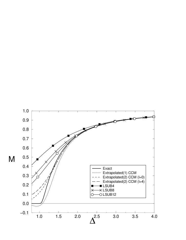
Figure 1:

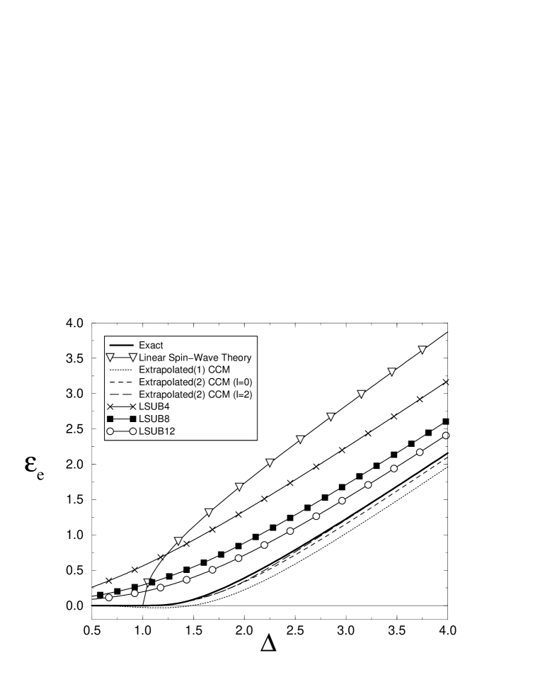
Figure 2:

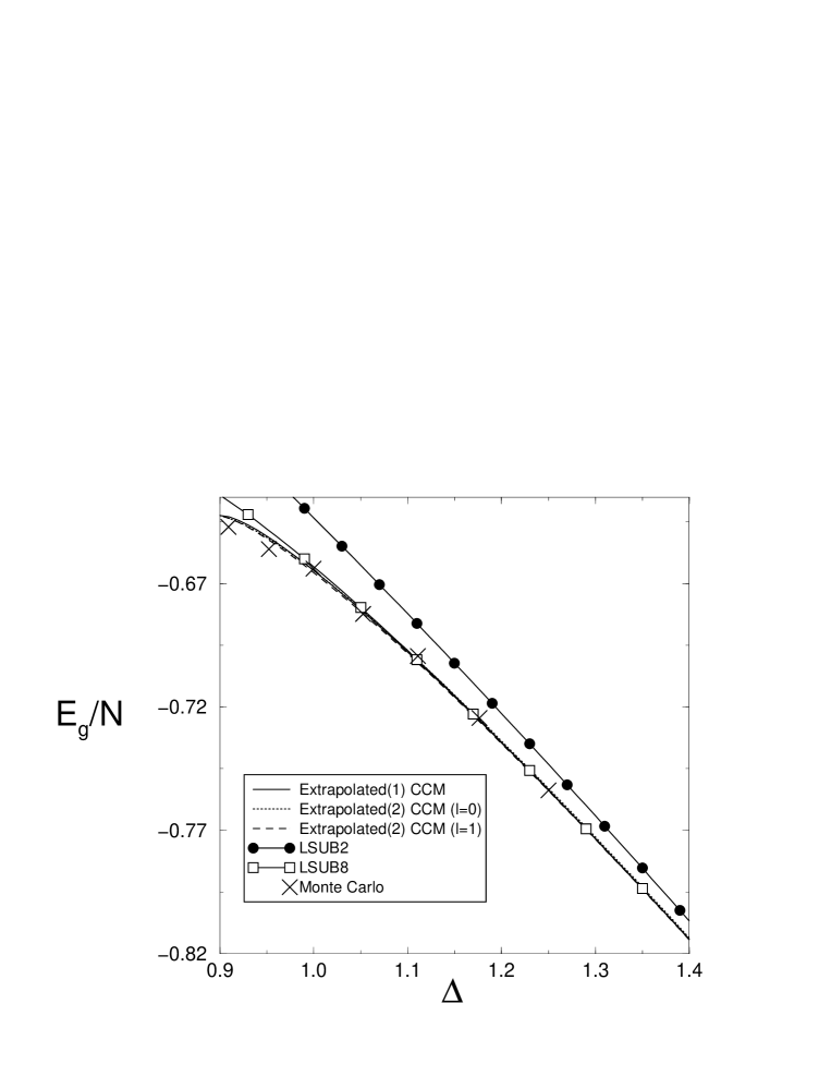
Figure 3:

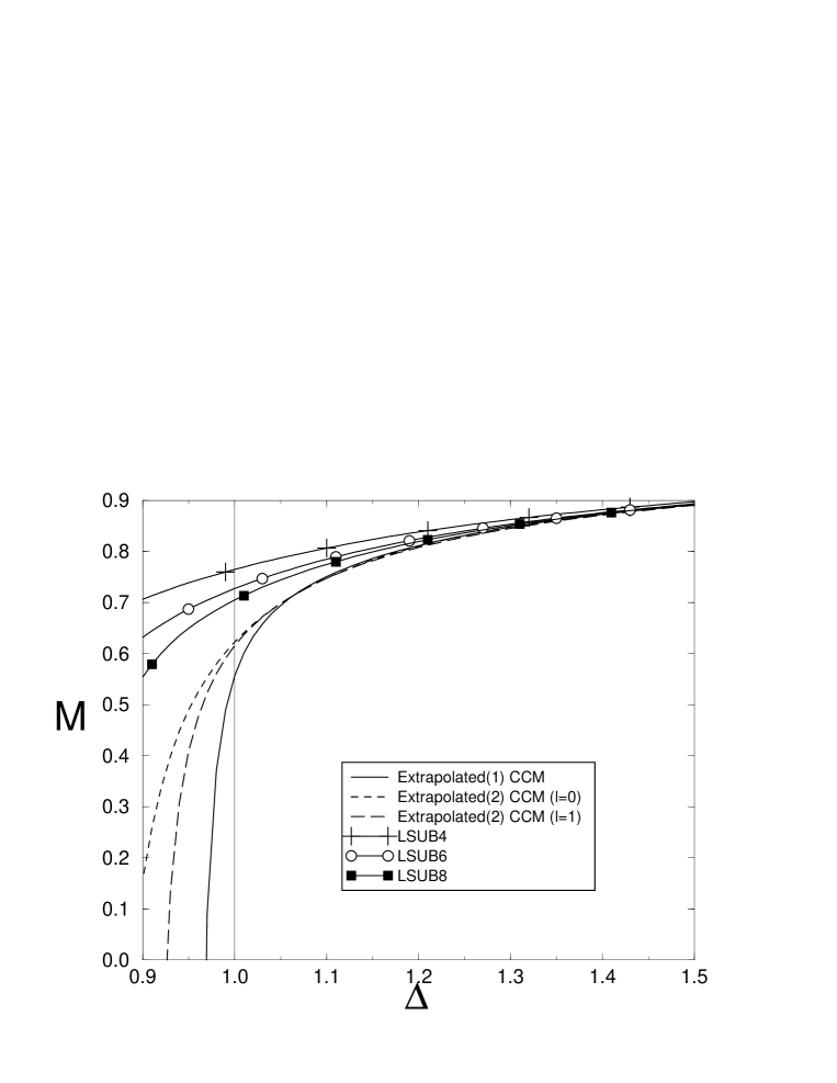
Figure 4:

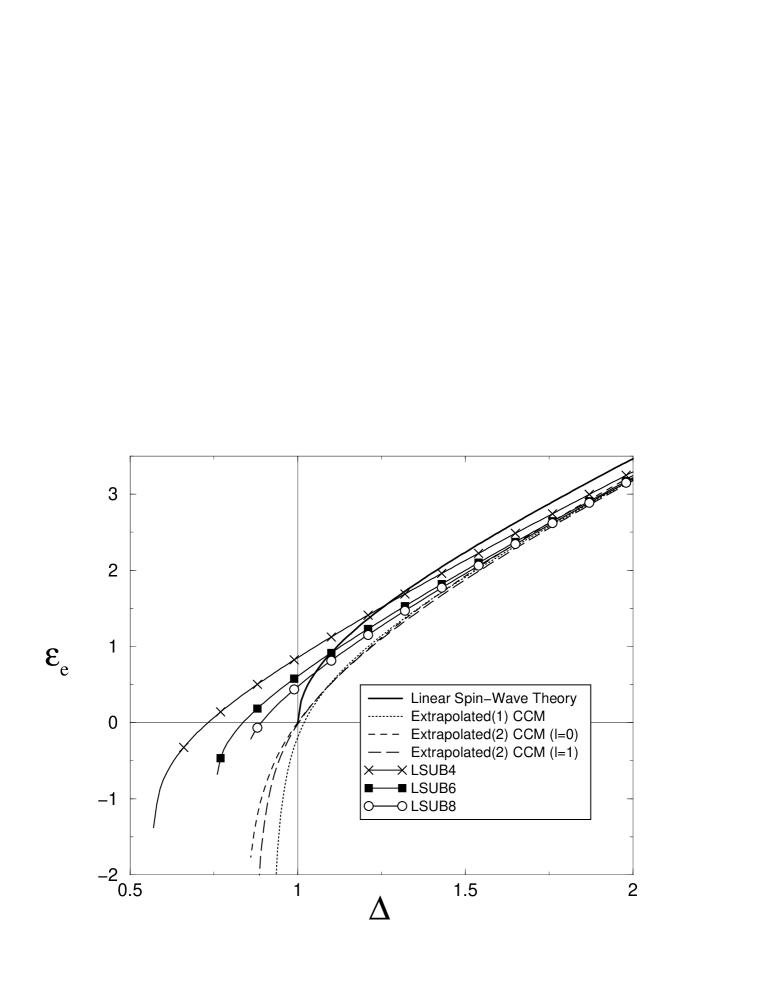
Figure 5:

References

- (1) F. Coester, Nucl. Phys. 7, 421 (1958); F. Coester and H. Kümmel, ibid. 17, 477 (1960).
- (2) H. Kümmel, K.H. Lührmann, and J.G. Zabolitzky, Phys Rep. 36C, 1 (1978).
- (3) R.F. Bishop and K.H. Lührmann, Phys. Rev. B 17, 3757 (1978).
- (4) J.S. Arponen, Ann. Phys. (N.Y.) 151, 311 (1983).
- (5) J.S. Arponen, R.F. Bishop, and E. Pajanne, Phys. Rev. A 36, 2519 (1987); ibid. 36, 2539 (1987); ibid. 37, 1065 (1988).
- (6) R.F. Bishop, Theor. Chim. Acta 80, 95 (1991).
- (7) J.S. Arponen, and R.F. Bishop, Ann. Phys. (N.Y.) 207, 171 (1991); ibid. 227, 275 (1993); ibid. 227, 2334 (1993).
- (8) R.F. Bishop, in Microscopic Quantum-Many-Body Theories and Their Applications, edited by J. Navarro and A. Polls, Lecture Notes in Physics, Vol. 510 (Springer-Verlag, Berlin, 1998), p. 1.
- (9) M. Roger and J.H. Hetherington, Phys. Rev. B 41, 200 (1990); M. Roger and J.H. Hetherington, Europhys. Lett. 11, 255 (1990).
- (10) R.F. Bishop, J.B. Parkinson, and Y. Xian, Phys. Rev. B 44, 9425 (1991).
- (11) R.F. Bishop, J.B. Parkinson, and Y. Xian, J. Phys.: Condens. Matter 5, 9169 (1993).
- (12) D.J.J. Farnell and J.B. Parkinson, J. Phys.: Condens. Matter 6, 5521 (1994).
- (13) Y. Xian, J. Phys.: Condens. Matter 6, 5965 (1994).
- (14) R. Bursill, G.A. Gehring, D.J.J. Farnell, J.B. Parkinson, T. Xiang, and C. Zeng, J. Phys.: Condens. Matter 7, 8605 (1995).
- (15) R.F. Bishop, R.G. Hale, and Y. Xian, Phys. Rev. Lett. 73, 3157 (1994); Int. J. Quantum Chem. 57, 919 (1996).
- (16) R.F. Bishop, D.J.J. Farnell, and J.B. Parkinson, J. Phys.: Condens. Matter 8, 11153 (1996).
- (17) D.J.J. Farnell, S.A. Krüger, and J.B. Parkinson, J. Phys.: Condens. Matter 9, 7601 (1997).
- (18) R.F. Bishop, Y. Xian, and C. Zeng, in Condensed Matter Theories, edited by E.V. Ludeña, P. Vashishta, and R.F. Bishop Vol. 11 (Nova Science Publ., Commack, New York, 1996), p. 91.
- (19) C. Zeng, D.J.J. Farnell, and R.F. Bishop, J. Stat. Phys., 90, 327 (1998).
- (20) R. F. Bishop, D.J.J. Farnell, and J.B. Parkinson, Phys. Rev. B 58, 6394 (1998).
- (21) R. F. Bishop, D. J. J. Farnell, and Chen Zeng, Phys. Rev. B 59, 1000 (1999).
- (22) J. Rosenfeld, N.E. Ligterink, and R.F. Bishop, Phys. Rev. B 60, 4030 (1999).
- (23) H. A. Bethe, Z. Phys. 71, 205 (1931).
- (24) L. Hulthén, Ark. Mat. Astron. Fys. A 26, No. 11 (1938).
- (25) R. Orbach, Phys. Rev. 112, 309 (1958); C. N. Yang and C. P. Yang, ibid. 150, 321 (1966); ibid. 150, 327 (1966).
- (26) J. Des Cloiseaux and Pearson, Phys. Rev. 128, 2131 (1962); L. D. Faddeev and L. A. Takhtajan, Phys. Lett. 85A, 375 (1981).
- (27) P. W. Anderson, Phys. Rev. 86, 694 (1952); T. Oguchi, Phys. Rev. 117, 117 (1960).
- (28) C.J. Hamer, Z. Weihong, P. Arndt, Phys. Rev. B 46, 6276 (1992).
- (29) S. Tang and J.E. Hirsch, Phys. Rev. B 39, 4548 (1989).
- (30) D. D. Betts and G. E. Stewart, Can. J. Phys. 75, 47 (1997).
- (31) W. Zeng, J. Oitmaa, and C. J. Hamer, Phys. Rev. B 43, 8321 (1991).
- (32) T. Barnes, D. Kotchan, and E. S. Swanson, Phys. Rev. B 39, 4357 (1989).
- (33) J. Carlson, Phys. Rev. B 40, 846 (1989); N. Trivedi and D. M. Ceperley, ibid. 41, 4552 (1990).
- (34) K. J. Runge, Phys. Rev. B 45, 12292 (1992); ibid. 45, 7229 (1992).
- (35) A.W. Sandvik, Phys. Rev. B 56, 11678 (1997).
- (36) K. Emrich, Nucl. Phys. A351, 379, 397 (1981).