Numerical analysis of the magnetic-field-tuned superconductor-insulator transition in two dimensions

Abstract

Ground state of the two-dimensional hard-core-boson model subjected to external magnetic field and quenched random chemical potential is studied numerically. In experiments, magnetic-field-tuned superconductor-insulator transition has already come under through investigation, whereas in computer simulation, only randomness-driven localization (with zero magnetic field) has been studied so far: The external magnetic field brings about a difficulty that the hopping amplitude becomes complex number (through the gauge twist), for which the quantum Monte-Carlo simulation fails. Here, we employ the exact diagonalization method, with which we demonstrate that the model does exhibit field-tuned localization transition at a certain critical magnetic field. At the critical point, we found that the DC conductivity is not universal, but is substantially larger than that of the randomness-driven localization transition at zero magnetic field. Our result supports recent experiment by Marković et al. reporting an increase of the critical conductivity with magnetic field strengthened.

PACS: 74.76.w Superconducting films, 71.23.An Theories and models; localized states, 75.40.Mg Numerical simulation studies, 68.35.Rh Phase transitions and critical phenomena, 75.10.Nr Spin-glass and other random models.

Keywords: magnetic-field-tuned superconductor-insulator transition, exact-diagonalization method, randomness, critical conductivity, dynamical critical exponent, finite-size-scaling method.

1 Introduction

Scaling argument of Abrahams, Anderson, Licciardello and Ramakrishnan [1] states that in two dimensions, infinitesimal amount of quenched randomness should drive itinerant extended states to localize. That is, at absolute zero temperature, the conductivity should vanish, if there exist any randomnesses. There are, however, some exceptions where the above description fails. Metal-insulator transition found in MOSFET devise [2, 3, 4], for instance, is one of recent hot topics arousing much attention. In the above-mentioned scaling theory, the randomness perturbation appears to be marginal so that some unexpected factors, for example, many-body interaction and external magnetic field, would possibly change the scenario.

Suppose that there exists an attractive interaction among particles. At the ground state,the particles would be unstable against bose condensation so that the system would fall into a superconducting state. Localization transition from the superconducting state is apparently out of the scope of the conventional localization theory, and has been studied extensively so far: In experiments, the transition is observed for metallic films [5, 6, 7, 8, 9] and Josephson-junction arrays [10, 11]. In essence, ${}^{4}{\rm He}$ film adsorbed by porous media belongs to the same physics as well [12, 13, 14], although one cannot measure its electronic conductivity. One of the main concerns, particularly in experiments, would be the conductivity at the localization point. An argument claims that localization transition occurs at a universal condition [18]. That is, at the transition point, irrespective of the samples examined, the electrical conductivity stays $\approx(2e)^{2}/h$ with the electron charge $e$ and the Plank constant $h$. A great number of experiments are trying to validate this issue. From theoretical view point, the criticality itself is a matter of interest [15, 16, 17, 18]. It is to be stressed that the localization transition occurs at the ground state (zero temperature). Such ground-state criticality differs significantly from that of the finite-temperature transitions, and belongs to a peculiar universality class: From the path-integral viewpoint for the partition function, $d$-dimensional quantum system is regarded as a $(d+1)$-dimensional classical system. The system size along the imaginary-time direction is given by the inverse temperature, which diverges at zero temperature. Critical fluctuation along the imaginary-time direction (quantum fluctuation) contributes to the nature of critical phenomenon, giving rise to a new universality class. This extra contribution is characterized by the dynamical critical exponent $z$; a formal scaling argument on the superconductor-insulator transition will be found in the literatures [16, 17]. We stress that such arguments on criticality are not of mere theoretical interest, but are readily measurable in experiments; see Table 1.

In order to tune the localization transition, either magnetic field strength or amount of randomness (film thickness) has to be adjusted carefully. Because the former is far more advantageous for fine tuning, numerous experiments are devoted to the magnetic-field-tuned localization transition. In Table 1, we presented a summary of experimental results. Among them, we would like to draw reader’s attention to the recent experiment by Marković et al. [25, 26], who scanned both two tuning parameters fairly systematically.

While in experiments, such the subtle issues have already come under through investigation, in computer simulation, on the contrary, it has not yet been done to incorporate the external magnetic field: So far, transitions driven solely by the random chemical potential (with zero magnetic field) have been simulated [27, 28, 29, 30, 31, 32, 33]. Implementation of the magnetic field brings about a complication such that the hopping amplitude becomes complex number. Because of this, quantum Monte-Carlo simulation does not work; the inefficiency would be even more serious than that of the so-called negative sign problem. (Note that here, the magnetic field is not meant to couple to the moment of spin (as in usual spin models), but it rather couples to the charge (hopping) through the gauge twist.) Simulation of ref. [34] is actually dealing with both magnetic field and randomness. In the model, however, the randomness is not of random chemical potential, but is of random hopping strength; the latter may lie rather out of present scope: Note that the chemical potential term (particle number) and the superconductivity order parameter (gauge) are conjugate variables. Co-existence of these mutually conjugate terms is the source of fascination of this physics. On the contrary, it causes the aforementioned technical complications.

Here, in order to overcome the difficulty of, so to speak, ‘complex-sign problem,’ we employed the exact-diagonalization method. This method has not been used so frequently in the course of the studies on this issue. Perhaps, the limitation of the tractable system sizes had been worried over. Yet, recent extensive simulations and subsequent careful data analyses are guaranteeing its validity and usefulness [27, 33]. In particular, the exact diagonalization has an advantage over others that the method gives dynamical response functions [35] such as the AC conductivity (without resorting to the maximum-entropy method, for instance). Of course, it does manage the complex Hamiltonian elements.

The rest of this paper is organized as follows. In the next section, we explain our model Hamiltonian of the two-dimensional hard-core-boson model with magnetic field and random chemical potential. Details how we had chosen the gauge will be explicated there. In Section 3, we present numerical results. For the first time, with use of the finite-size-scaling method, we observe clear evidences of the onset of field-tuned localization transition. After determining the transition point, we evaluate experimentally accessible quantities such as the critical conductivity and the dynamical critical exponent. The last section is devoted to summary and discussions.

2 Model Hamiltonian — two-dimensional hard-core-boson model

In this section, we explain our model Hamiltonian and some of its physical ingredients. The model we simulated is the hard-core-boson model on the square lattice subjected to external magnetic field and quenched random chemical potential. The Hamiltonian is given by,

$${\cal H}=-\frac{J}{2}\sum_{\langle ij\rangle}\left({\rm e}^{{\rm i}\phi_{ij}}b^{\dagger}_{i}b_{j}+{\rm e}^{-{\rm i}\phi_{ij}}b^{\dagger}_{j}b_{i}\right)+\sum_{i}H_{i}(2b^{\dagger}_{i}b_{i}-1).$$ (1)

$\sum_{\langle ij\rangle}$ denotes the summation over all nearest neighbors on the square lattice of size $L\times L$. Periodic-boundary condition is imposed as for the horizontal ($x$-axis) direction. The operators $\{b_{i}\}$ ($\{b^{\dagger}_{i}\}$) are the hard-core-boson annihilation (creation) operators at site $i$. The gauge twist angles $\{\phi_{ij}\}$ are chosen such as $\phi_{ij}=(i_{y}-(L+1)/2)\pi B$ for the horizontal $i$-$j$ pair of $j$ right next to $i$, and $\phi_{ij}=0$ for the vertical $i$-$j$ pair. Because of this choice of gauge, a particle hopping clockwise around a plaquette feels, as a whole, the gauge angle of $\pi B$. That is, the bosons are subjected to the uniform magnetic flux $\pi B$ per plaquette. Hereafter, we call $B$ ‘magnetic field.’ (Therefore, the situation of half flux quantum per plaquette is realized at the magnetic-field strength $B=1$.) Quenched random chemical potentials $\{H_{i}\}$ distribute over the sector $[-\sqrt{3}\Delta,\sqrt{3}\Delta]$ uniformly (rectangular distribution). Therefore, the strength of randomness is controlled by the parameter $\Delta=[H_{i}^{2}]_{\rm av}$, where $[\cdots]_{\rm av}$ denotes the random-sample average.

Let us try to transcribe the situation realized by the Hamiltonian (1) in a manner appealing our intuition more vividly: Hard-core bosons are confined in a square lattice. Throughout this paper, we fix the particle density to be half-filled. In the absence of $B$ and $\Delta$, a statistical mechanical theorem ensures that the particles are superconducting (namely, the gauge symmetry is broken spontaneously) at the ground state [36]; note that because of the hard-core restriction, the onset of superconductivity is a subtle issue. The random chemical potential $\{H_{i}\}$ may work so as to disturb the superconductivity. The strength of the randomness is preferably slightly less than that of the localization-transition threshold, and so the bosons are left still superconducting. Because the horizontal periodic boundary condition is imposed, the lattice is rolled up to form a cylinder. From each end of the cylinder, two bar magnets are inserted so that the cylinder is subjected to magnetic field perpendicular to the cylinder surface. This magnetic field is supposed to destroy the superconductivity so that Anderson localization may occur at a certain critical magnetic field eventually. This magnetic-field-swept transition has not yet been simulated, whereas the randomness-driven transition has already been simulated extensively [27, 28, 29, 30, 31, 32, 33]. For a summary of preceding simulation results at $B=0$, readers may consult with Introduction of ref. [33].

It is meaningful to transform the boson Hamiltonian (1) into the form of quantum $XX$ model. With use of the mapping relations between hard-core boson and $S=1/2$ spin [37],

$$b_{i}^{\dagger} = S^{+}_{i}$$

$$b_{i} = S^{-}_{i},$$ (2)

the above Hamiltonian (1) is expressed in terms of the $S=1/2$ spin operators,

$${\cal H}=-\frac{J}{2}\sum_{\langle ij\rangle}\left({\rm e}^{{\rm i}\phi_{ij}}S^{+}_{i}S^{-}_{j}+{\rm e}^{-{\rm i}\phi_{ij}}S^{-}_{i}S^{+}_{j}\right)+2\sum_{i}H_{i}S^{z}_{i},$$ (3)

apart from a constant term. Now, we are in a position to address some notions gained from this spin representation: The onset of superconductivity, that is, the spontaneous breaking of gauge symmetry, is interpreted as the appearance of the in-plane spontaneous magnetization; that is,

$$M_{XY}^{2}=\sum_{i\neq j}\left(S^{x}_{i}S^{x}_{j}+S^{y}_{i}S^{y}_{j}\right).$$ (4)

(In the above, the spin-spin correlations over the identical sites are subtracted, because they just yield a constant term. That subtraction improves finite-size-scaling behavior.) It is proved rigorously [36] that the in-plane symmetry is spontaneous broken at the ground state of the two-dimensional $XX$ model. Therefore, it is expected that at least in the vicinity of $B=0$ and $\Delta=0$, our system (1) may continue to be in a superconductor phase. The perturbations of $B$ and $\Delta$ are supposed to destroy the superconductivity. In the spin language, $B$ introduces in-plane magnetic frustration at each plaquette; experts at the quantum Monte-Carlo technique may be convinced now why the method does not work. On the other hand, $\Delta$ appears to be random magnetic field coupling the $z$-component of spin. In the next section, we will study how $M_{XY}$ gets disturbed by these perturbations numerically.

3 Numerical results

In this section, we present numerical results. We have performed exact-diagonalization calculation for the Hamiltonian (3) with system sizes up to $L=5$. We have fixed the particle density to be half-filled $n(=N/L^{2})=0.5$. For those system sizes of odd $L$, we carried out two sets of simulations for the particle numbers of $N=[L^{2}/2]$ and $[L^{2}/2]-1$ (the bracket $[\cdots]$ denotes the Gauss notation). Thereby, we performed interpolation calculation (least-square fitting) with respect to those data so as to obtain the data at $n=0.5$. In the interpolation, we used the relation $Q(n)=a(n-0.5)^{2}+c$, which means that the physics is symmetric with respect to $n=0.5$ (owing to the particle-hole symmetry). The amount of randomness $\Delta$ is kept unchanged throughout the simulation; namely, $\Delta=0.7$.

3.1 Field-tuned localization

In this subsection, we will show evidences of the superconductor-insulator transition tuned by the magnetic field. In the analysis, the spin language (3) is used. Namely, the localization transition is identified as the disappearance of the $XY$ (in-plane) magnetic order $M_{XY}$.

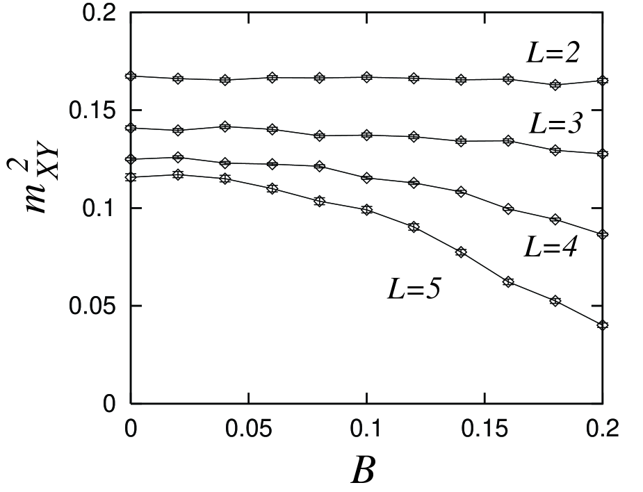
Figure 1: Square of the in-plane magnetization (superconductivity-order parameter) (4) is plotted for $\Delta=0.7$ and various $B$. From the plot, we see that the in-plane order gets disturbed gradually by the magnetic field $B$.

In Fig. 1, we plotted the square of the in-plane magnetization per site $m^{2}=[\langle M_{XY}^{2}\rangle]_{\rm av}/L^{4}$ for $\Delta=0.7$ and various $B$. The bracket $[\cdots]_{\rm av}$ denotes the random-sample average. $\langle\cdots\rangle$ denotes the ground-state expectation for respective random samples. The random-sample numbers are $1024$, $1024$, $1024$ and $192$ for $L=2$, $3$, $4$ and $5$, respectively. As is noted above, for odd $L$, we have performed two sets of simulations. Hence, the number of random samples is effectively twice as many as that indicated above for odd $L$. From the plot, we see that the in-plane magnetization gets suppressed by $B$. However, onset of localization transition seems to be less transparent. Indication of the localization transition will be seized in the following analyses.

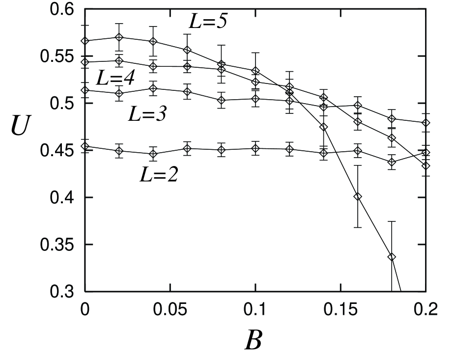
Figure 2: Binder parameter for the in-plane magnetic order (5) is plotted for the same parameter range as that of Fig. 1. The intersection point of the curves gives the location of the localization-transition point. Hence, we found that at $B\approx 0.1$, localization transition takes place.

In Fig. 2, we plotted the Binder parameter $U$ [38] for the in-plane magnetic order; that is,

$$U=1-\frac{[\langle M_{XY}^{4}\rangle]_{\rm av}}{3[\langle M_{XY}^{2}\rangle]_{\rm av}^{2}}.$$ (5)

Finite-size-scaling behavior of the Binder parameter contains information whether $M_{XY}$ develops or not: As $L$ is enlarged, the Binder parameter should grow (be suppressed), provided that the order $M_{XY}$ is long-ranged (short ranged). At critical point, it remains scale-invariant with respect to $L$. That is, intersection point of the Binder-parameter curves yields the location of the transition point.

From the plot, we see that an intersection point locates at $B\approx 0.1$. Namely, the superconductor phase survives up to the critical magnetic field $B\approx 0.1$, at which the field-tuned localization transition takes place eventually. However, rather large corrections to finite-size scaling, especially for small $L$, prevent precise determination of the critical point.

We carried out an alternative analysis so as to complement the above observation. We calculated the gauge stiffness $\Upsilon$ [39], which is defined by the elasticity with respect to the boundary gauge twist;

$$\Upsilon=\left[\left\langle\left.\frac{\partial^{2}E_{\rm g}(\Theta)}{\partial\Theta^{2}}\right|_{\Theta=0}\right\rangle\right]_{\rm av},$$ (6)

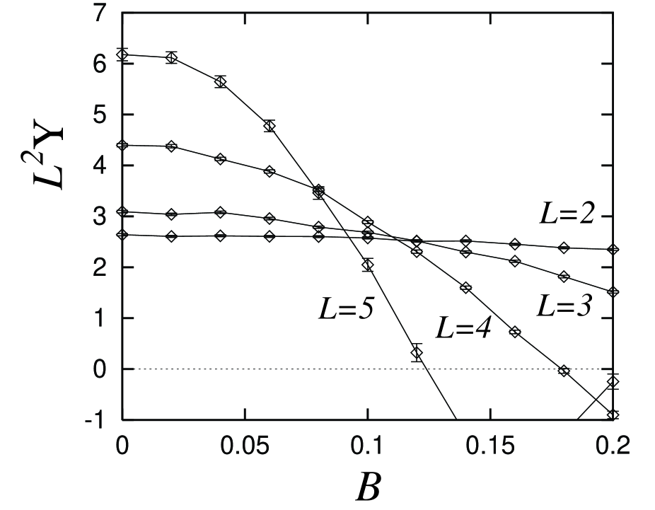
Figure 3: Scaled gauge stiffness (6) is plotted for the same parameter range as that of Fig. 1. The intersection point of the curves yields the critical point. Therefore, the estimate $B\approx 0.1$ of the former analysis of Fig. 2 is supported. In addition, it is suggested that $z=2$ holds. This relation will be confirmed in the subsequent analysis of Fig. 6.

where $\Theta$ denotes the gauge-twist angle through the periodic boundary, and $E_{\rm g}(\Theta)$ is the ground-state energy under the twisted boundary condition $\Theta$. In other words, $\Upsilon$ is the elasticity modulus against the introduction of a magnetic flux penetrating through the cylinder; note that our square lattice is rolled up to form a cylinder. Therefore, the stiffness should remain finite in the superconductor phase, while it vanishes in the Anderson-localization phase. In Fig. 3, we plotted the scaled stiffness $L^{2}\Upsilon$ for the same parameter range as that of Figs. 1 and 2. We observe that the stiffness is suppressed by $B$ as would be expected. In order to gain further information from this scaling plot, we have to consult with the formal scaling argument on $\Upsilon$ [16, 17]. According to this argument, at the localization point, the stiffness should obey the scaling relation $\Upsilon\sim L^{-(d+z-2)}$. That is, the scaled stiffness $L^{d+z-2}\Upsilon$ should be scale-invariant at the localization transition point. Actually, from the plot, we see that the scaled stiffness with the particular choice of $z=2$ exhibits scale invariance at critical point $B\approx 0.1$; the validity of $z=2$ will be confirmed in the analysis of Section 3.3. Putting together the finite-size-scaling behaviors of $U$ and $\Upsilon$, we are led to the conclusion that the field-tuned localization takes place at $B\approx 0.1$. In the following, we calculate experimentally accessible quantities at the point $B=0.1$.

3.2 Critical conductivity

Here, we evaluate the AC conductivity at the localization point $B=0.1$ determined in the above subsection. As is mentioned in Introduction, an argument claims that the DC conductivity would be a universal value of the order $\approx(e^{*})^{2}/h$ with charge of one particle $e^{*}$ (say, Cooper pair). Various experiments have tried to validate this issue. However, the results are still remaining controversial; see Table 1. Nevertheless, it should be noted that finite conductivity itself is a novel feature lying out of the scope of the conventional localization theory in two dimensions; see Introduction.

According to the Kubo formula, the AC conductivity is expressed in terms of the current-current correlation function,

$$\sigma(\omega)={\rm Re}\left[\frac{1}{\hbar\omega L^{2}}\int_{0}^{\infty}{\rm d}t{\rm e}^{{\rm i}\omega t}\left\langle\left[J_{x}(t),J_{x}\right]\right\rangle\right]_{\rm av},$$ (7)

with the current operator $J_{x}=\frac{{\rm i}e^{*}J}{2\hbar}\sum_{j,\delta_{x}}{\rm e}^{{\rm i}\phi_{j,j+\delta_{x}}}\delta_{x}a_{j+\delta_{x}}^{\dagger}a_{j}$. This formula reduces to the resolvent form,

$$\sigma(\omega)={\rm Re}\left(\frac{{\rm i}}{\hbar\omega L^{2}}\left[\left\langle J_{x}\left(\frac{\hbar}{E_{\rm g}-{\cal H}+\hbar\omega+{\rm i}\eta}+\frac{\hbar}{E_{\rm g}-{\cal H}-\hbar\omega-{\rm i}\eta}\right)J_{x}\right\rangle\right]_{\rm av}\right).$$ (8)

Hence, one is forced to calculate the inverse of the Hamiltonian matrix, which is seemingly impossible in practice. However, Gagliano and Balseiro found that the resolvent is expanded into the following continued-fraction form [35],

$$\left\langle f_{0}\left|\frac{1}{z-{\cal H}}\right|f_{0}\right\rangle=\frac{\langle f_{0}|f_{0}\rangle}{z-\alpha_{0}-\frac{\beta_{1}^{2}}{z-\alpha_{1}-\frac{\beta_{2}^{2}}{\ddots}}},$$ (9)

with the coefficients generated by the following recursion relations,

$$|f_{i+1}\rangle = {\cal H}|f_{i}\rangle-\alpha_{i}|f_{i}\rangle-\beta_{i}^{2}|f_{i-1}\rangle,$$

$$\alpha_{i} = \langle f_{i}|{\cal H}|f_{i}\rangle/\langle f_{i}|f_{i}\rangle,$$

$$\beta_{i}^{2} = \langle f_{i}|f_{i}\rangle/\langle f_{i-1}|f_{i-1}\rangle\ \ (\beta_{0}=0).$$ (10)

These procedures are essentially the same as those of the Lanczos tri-diagonalization. It is one of major advantages of the Lanczos diagonalization that one can calculate dynamical response functions.

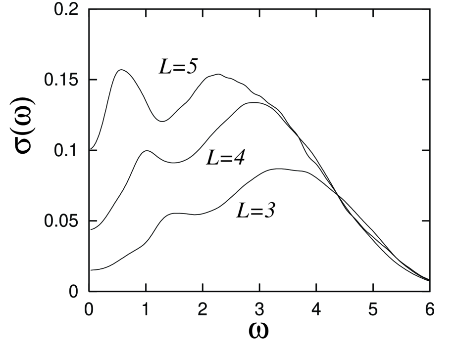
Figure 4: AC conductivity at the localization-transition point ($\Delta=0.7$ and $B=0.1$) is plotted. Rapid drop in the vicinity of $\omega=0$ is due to the finite-size effect. Hence, the maximal conductivity beside $\omega=0$ has to be regarded as the DC conductivity for each $L$.

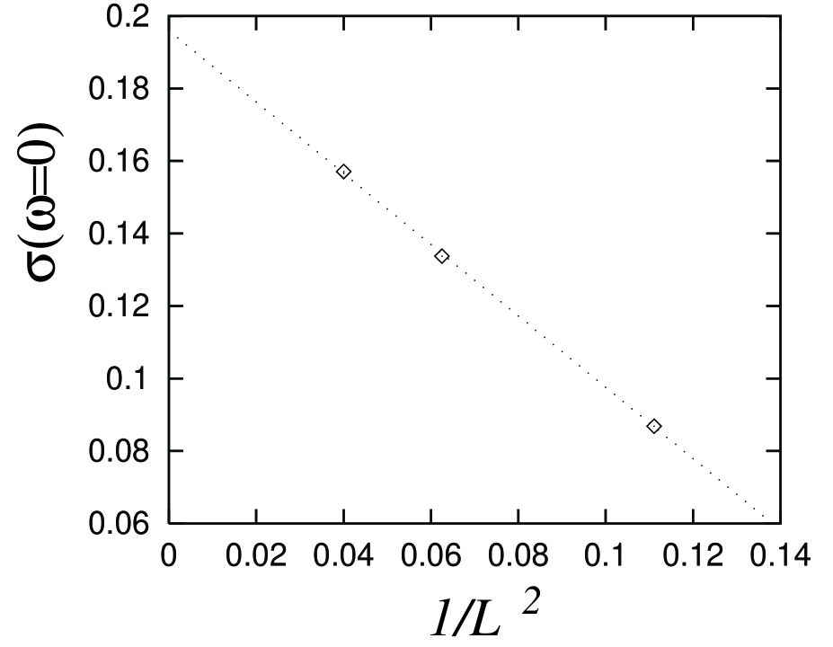
Figure 5: DC conductivity at the localization-transition point ($\Delta=0.7$ and $B=0.1$) is plotted against $1/L^{2}$. Through the least-square fit, we obtained the critical DC conductivity in the $L\to\infty$ limit as $\sigma_{\rm c}=0.196\pm 0.01((e^{*})^{2}/h)$. This value turns out to be substantially larger than that of the randomness-driven transition $\sigma_{\rm c}\approx 0.135((e^{*})^{2}/h)$ at $B=0$.

In Fig. 4, we plotted the AC conductivity at the transition point ($B=0.1$ and $\Delta=0.7$); we had set $\eta=0.2$. The data are averaged over random samples of $1024$, $1024$ and $64$ for $L=3$, $4$ and $5$, respectively. Because of finite-size energy gap above the ground state, the AC conductivity in Fig. 4 drops in the vicinity of $\omega=0$. AC conductivity curve forms a peak beside $\omega=0$, and as $L$ is enlarged, the peak position shifts toward the center $\omega=0$. Hence, for sufficiently large system sizes, the drop of $\sigma(\omega\approx 0)$ may disappear, and a Drude-like peak centered at $\omega=0$ may emerge instead. Therefore, we regard the maximal conductivity beside $\omega=0$ as the DC conductivity for respective $L$. Since the DC conductivity for each $L$ exhibits finite-size correction, we need to extrapolate those finite-$L$ data to the value of thermodynamic limit. In Fig. 5, we plotted the finite-$L$ DC conductivity against $1/L^{2}$; the choice of this abscissa scale is due to the reasoning addressed in the literature [27]. Through the least-square fit, we obtained the DC conductivity in the thermodynamic limit such as $\sigma_{\rm c}=0.196\pm 0.001((e^{*})^{2}/h)$. Remarkably enough, we notice that this conductivity is larger than that of the randomness-driven transition $\sigma_{\rm c}\approx 0.135((e^{*})^{2}/h)$ at $B=0$ [33], suggesting breakdown of the universality of $\sigma_{\rm c}$. We will discuss this point in the last section.

3.3 Dynamical critical exponent

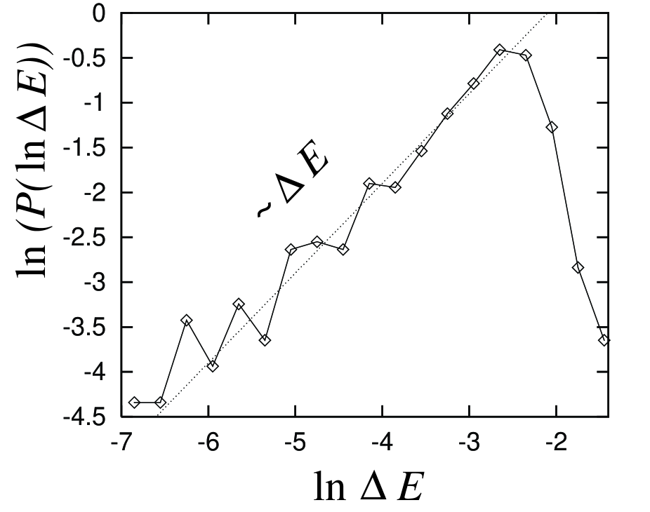
Figure 6: Probability distribution of $\log$ of the first energy gap over $512$ random samples with $L=5$ at the localization-transition point ($\Delta=0.7$ and $B=0.1$). The dotted line shows the slope of $P\sim\Delta E$. From the low-energy tail of this distribution, we obtain an estimate of the dynamical critical exponent $z=2$.

In the subsection 3.1, we have already used the relation $z=2$ for the purpose of investigating scaling property of the gauge stiffness $\Upsilon$ (6). In this subsection, we obtain more conclusive estimate of $z$ with use of the Rieger-Young relation [40]. In Fig. 6, we show the probability distribution of the logarithm of the first energy gap $\log\Delta E$ over $512$ random samples with $L=5$ at the transition point ($B=0.1$ and $\Delta=0.7$). According to the Rieger-Young argument, the low-energy tail of the distribution contains an information of the dynamical critical exponent. In the following, we recollect their argument briefly. Because our system is disordered, the first energy gap $\Delta E$ distributes obeying a certain probability-distribution function $P$. We are considering critical phenomenon, where the physics is scale-invariant and no such particular energy scale that characterize the physics exists. Therefore, it is sensible to consider $P(\log\Delta E)$ rather than $P(\Delta E)$. Low-lying excitation may be created at a peculiar part of random sample, where local excitation costs very little energy. Therefore, the probability may be proportional to the spatial volume; namely, $P\propto L^{d}\Delta E^{\lambda}$ with the exponent $\lambda$ describing the low-energy tail. On the other hand, the finite-size-scaling theory insists that it should be of the form $P=\tilde{P}(L/\xi_{\rm r})=\tilde{P}(L/\xi_{\tau}^{1/z})$ (definition of $z$). With use of the relation $\Delta E\sim 1/\xi_{\tau}$, the distribution turns out to be a function of $L(\Delta E)^{1/z}$. Therefore, we obtain the relation,

$$\log P(\log\Delta E)=\lambda\log\Delta E+C,$$ (11)

with $\lambda=d/z$.

In Fig. 6, we observe that the low-energy tail is, in fact, governed by that scaling relation with the exponent $\lambda=1$. In consequence, we obtain the relation $z=d=2$, confirming the preliminary estimate obtained in the subsection 3.1.

4 Summary and discussions

We have simulated the two-dimensional hard-core-boson model (1) subjected to the external magnetic field and the random chemical potential $\Delta=0.7$. Difficulty arising from the complex hopping amplitudes $\{{\rm e}^{{\rm i}\phi_{ij}}\}$, that have been preventing the application of the quantum Monte-Carlo method, is circumvented by the use of the exact-diagonalization scheme. For the first time, in computer simulation, we observed evidences of the field-tuned localization transition with the finite-size-scaling technique applied to the gauge order $M_{XY}$ as well as the gauge stiffness $\Upsilon$. After determining the location of the localization point, we carried out calculations of two experimentally accessible quantities, namely, the critical conductivity and the dynamical critical exponent. Thereby, we obtained those estimates such as $\sigma_{\rm c}=0.196\pm 0.01((e^{*})^{2}/h)$ and $z=2$. First, let us make a comparison with preceding simulation results. Although no former results for $B\neq 0$ are available, there have been reported a number of simulation studies at $B=0$ [27, 28, 29, 30, 31, 32, 33]. These simulation results are settling gradually to the conclusions such as $\sigma_{\rm c}\approx 0.135((e^{*})^{2}/h)$ and $z=2$. Hence, contrary to common belief, we are led to conclude that the critical conductivity is not universal but increases as the external magnetic field is strengthened. As for $z$, on the other hand, we found that the dynamical critical exponent $z=2$ is retained even for $B\neq 0$.

Secondly, let us turn our attention to making a comparison with experiments. As is noted above, the quantities evaluated here are measurable in experiments; a summary of experimental results is presented in Table 1. Among various reports listed there, in particular, we would like to draw reader’s attention to the latest exhaustive measurement by Marković et al. [25, 26], who scanned both magnetic-field strength and film thickness (randomness). Their experiment demonstrates that the critical conductivity (resistivity) does not stay universal but increases (decreases) gradually as $B$ is applied. Our numerical result supports this behavior [23, 25, 26]. Non-universality of $\sigma_{\rm c}$ has been arousing much attention. Meanwhile, there have been proposed several ideas intending to account for that [41, 42, 43, 44, 45, 46, 47]; for instance, it was proposed that one should take into account dissipative modes (possibly un-paired normal electrons) that would give rise to extra resistivity in addition to the intrinsic one. Our result shows, however, that without resorting to such dissipative extra modes, one can account for the gradual increase of $\sigma_{\rm c}$ within the framework of the pure-boson model (1). As for $z$, it appears that the numerical simulation result $z=2$ is not in agreement with experiments. The discrepancy had already come out in the past studies of $B=0$. There had been proposed an attempt at altering the universality class [30, 31]; It was claimed that an inclusion of long-range repulsion among particles would alter the universality class. Because in our exact-diagonalization calculation, tractable system sizes might not be sufficient to implement long-range interaction, it would be exceedingly cumbersome to validate this issue definitely.

In preliminary stage of our simulation, we had swept various parameter ranges so as to find optimal condition to observe localization transition: Note that $\Delta$ should not exceed a threshold at which particles localize already at zero magnetic field $B=0$. On the other hand, $\Delta$ should not be too weak, because superconductor-insulator transition may occur at strong magnetic field ($B\sim 0.5$). For such $B$ in close proximity to some primal fractional numbers, certain specific type of vortex-lattice structure becomes favored so that simulation data with sweeping magnetic field suffer from insystematic behaviors. Moreover, for large $B$, one cannot judge at all whether superconductivity is destroyed solely by the magnetic field or assistance of randomness is also significant. After sweeping various parameter ranges, we had determined the optimal randomness $\Delta=0.7$, and thereby, we performed extensive simulations at this particular condition. It would be remained for future study to gain inclusive features for the whole region including strong magnetic field.

Reference	Sample	Critical exponents	Critical resistivity
Hebard et al. [19]	${\rm InO}_{x}$ film	$z\approx 1$, $z\nu\approx 1.3$	$5000\Omega$
Tanda et al. [20]	High-$T_{\rm c}$ film	$z\nu=1.2(1)$	$8.5{\rm k}\Omega$
Seidler et al. [21]	High-$T_{\rm c}$ film	$z\nu=1.37(10)$	$13.6{\rm k}\Omega$
Chen et al. [22]	JJ array	$z\nu=1.5\sim 8$,	non-universal
		$z=1.05$
Yazdani et al. [23]	MoGe film	$\nu\approx 1.5$, $z=1.0(1)$	$R_{\Box}\downarrow$ as $B_{\rm c}\uparrow$
van der Zant et al. [24]	JJ array	$z\nu=1.2\sim 2$,	non-universal
		$z=0.34\sim 1.4$
Marković et al. [25, 26]	Bismuth film	$z\approx 1$, $\nu\approx 0.7$	$R_{\Box}\downarrow$ as $B_{\rm c}\uparrow$

Table 1: A summary of previous experimental measurements. Because even in a single literature, a number of different data are presented for respective samples, we have presented above a mean value.

References

- [1] E. Abrahams, P. W. Anderson, D. C. Licciardello and T. V. Ramakrishnan: Phys. Rev. Lett. 42 (1979) 673.
- [2] S. V. Kravchenko, G. V. Kravchenko, J. E. Furneaux, V. M. Pudalov and M. D’Iorio: Phys. Rev. B 50 (1994) 8039.
- [3] S. V. Kravchenko, W. E. Mason, G. E. Bowker, J. E. Furneaux, V. M. Pudalov and M. D’Iorio: Phys. Rev. B 51 (1995) 7038.
- [4] S. V. Kravchenko, D. Simonian, M. P. Sarachik, W. Mason and J. E. Furneaux: Phys. Rev. Lett. 77 (1996) 4938.
- [5] D. B. Haviland, Y. Liu, A. M. Goldman: Phys. Rev. Lett 62 (1989) 2180.
- [6] Y. Liu, K. A. McGreer, B. Nease, D. B. Haviland, G. Martinez, J. W. Halley and A. M. Goldman: Phys. Rev. Lett. 67 (1991) 2068.
- [7] S. J. Lee and J. B. Ketterson: Phys. Rev. Lett. 64 (1990) 3078.
- [8] A. F. Hebard and M. A. Paalanen: Phys. Rev. Lett. 54 (1985) 2155.
- [9] T. Wang, K. M. Beauchamp, D. D. Berkley, B. R. Johnson, J.-X. Liu, J. Zhang and A. M. Goldman: Phys. Rev. B 43 (1991) 8623.
- [10] L. J. Geerligs, M. Peters. L. E. M. de Groot, A. Verbruggen and J. E. Mooji: Phys. Rev. Lett. 63 (1989) 326.
- [11] S. Katsumoto: J. Low Temp. Phys. 98 (1995) 287.
- [12] B. C. Crooker, B. Hebral, E. N. Smith, Y. Takano and J. D. Reppy: Phys. Rev. Lett. 51 (1983) 666.
- [13] D. Finotello, K. A. Gillis, A. Wong and M. H. Chan: Phys. Rev. Lett. 61 (1988) 1954.
- [14] P. A. Crowell, F. W. van Keuls and J. D. Reppy: Phys. Rev. B 55 (1997) 12620, and references therein.
- [15] M. Ma, B. I. Halperin and P. A. Lee: Phys. Rev. B 34 (1986) 3136.
- [16] M. P. A. Fisher, P. B. Weichman, G. Grinstein and D. S. Fisher: Phys. Rev. B. 40 (1989) 546.
- [17] M. P. A. Fisher, G. Grinstein and S. M. Girvin: Phys. Rev. Lett. 64 (1990) 587.
- [18] M. P. A. Fisher: Phys. Rev. Lett. 65 (1990) 923.
- [19] A. F. Hebard and M. A. Paalanen: Phys. Rev. Lett. 65 (1990) 927.
- [20] S. Tanda, S. Ohzeki and T. Nakayama: Phys. Rev. Lett. 69 (1992) 530.
- [21] G. T. Seidler, T. F. Rosenbaum and B. W. Veal: Phys. Rev. B 45 (1992) 10162.
- [22] C. D. Chen, P. Delsing, D. B. Haviland, Y. Harada and T. Claeson: Phys. Rev. B 51 (1995) 15645.
- [23] A. Yazdani and A. Kapitulnik: Phys. Rev. Lett. 74 (1995) 3037.
- [24] H. S. J. van der Zant, W. J. Elion, L. J. Geerligs and J. E. Mooij: Phys. Rev. B 54 (1996) 10081.
- [25] N. Marković, C. Christiansen and A. M. Goldman: Phys. Rev. Lett. 81 (1998) 5217.
- [26] N. Marković, C. Christiansen, A. M. Mack, W. H. Huber and A. M. Goldman: Phys. Rev. B 60 (1999) 4320.
- [27] K. J. Runge: Phys. Rev. B 45 (1992) 13136.
- [28] M. Makivić, N. Trivedi and S. Ullah: Phys. Rev. Lett. 71 (1993) 2307.
- [29] G. G. Batrouni, B. Larson, Scalettar, Tobochnik and Wang: Phys. Rev. B 48 (1993) 9628.
- [30] M. Wallin, E. S. Sørensen, S. M. Girvin and A. P. Young: Phys. Rev. B 49 (1994) 12115.
- [31] E. S. Sørensen, M. Wallin, S. M. Girvin and A. P. Young: Phys. Rev. Lett. 69 (1992) 828.
- [32] S. Zhang, N. Kawashima, J. Carlson and J. E. Gubernatis: Phys. Rev. Lett. 74 (1995) 1500.
- [33] Y. Nishiyama: Eur. Phys. J B 9 (1999) 215.
- [34] M.-C. Cha and S. M. Girvin: Phys. Rev. B 49 (1994) 9794.
- [35] E. R. Gagliano and C. A. Balseiro: Phys. Rev. Lett. 59 (1987) 2999.
- [36] T. Kishi and K. Kubo: J. Phys. Soc. Japan 58 (1989) 2547.
- [37] T. Matsubara and H. Matsuda: Prog. Theor. Phys. 16 (1956) 569.
- [38] K. Binder: Phys. Rev. Lett. 47 (1981) 693.
- [39] M. E. Fisher, M. N. Barber and D. Jasnow: Phys. Rev. A 8 (1973) 1111.
- [40] H. Rieger and A. P. Young: Phys. Rev. B 54 (1996) 3328.
- [41] E. Shimshoni, A. Auerbach and A. Kapitulnik: Phys. Rev. Lett. 80 (1998) 3352.
- [42] N. Mason and A. Kapitulnik: Phys. Rev. Lett. 82 (1999) 5341.
- [43] K.-H. Wagenblast, A. van Otterlo, G. Schön and G. T. Zimányi: Phys. Rev. Lett. 79 (1997) 2730.
- [44] A. Krämer and S. Doniach: Phys. Rev. Lett. 81 (1998) 3523.
- [45] A. J. Rimberg, T. R. Ho, C. Kurdak, J. Clarke, K. L. Campman and A. C. Gossard: Phys. Rev. Lett. 78 (1997) 2632.
- [46] N. Trivedi, R. T. Scalettar and M. Randeria: Phys. Rev. B 54 (1996) 3756.
- [47] C. Huscroft and R. T. Scalettar: Phys. Rev. Lett. 81 (1998) 2775.