High–momentum dynamic structure function of liquid ³He–⁴He mixtures: a microscopic approach

Abstract

The high-momentum dynamic structure function of liquid ³He-⁴He mixtures has been studied introducing final state effects. Corrections to the impulse approximation have been included using a generalized Gersch-Rodriguez theory that properly takes into account the Fermi statistics of ³He atoms. The microscopic inputs, as the momentum distributions and the two-body density matrices, correspond to a variational (fermi)-hypernetted chain calculation. The agreement with experimental data obtained at $q=23.1$ Å^-1 is not completely satisfactory, the comparison being difficult due to inconsistencies present in the scattering measurements. The significant differences between the experimental determinations of the ⁴He condensate fraction and the ³He kinetic energy, and the theoretical results, still remain unsolved.

I INTRODUCTION

Liquid ³He-⁴He mixtures at low temperature have been of long-standing interest from both experimental[1, 2] and theoretical[3, 4, 5] viewpoints. From the theoretical side, isotopic ³He-⁴He mixtures manifest fascinating properties intrinsically related to their quantum nature. The different quantum statistics of ⁴He (boson) and ³He (fermion) appear reflected in the macroscopic properties of the mixture as its very own existence in the zero-temperature limit. One of the most relevant features that the ³He-⁴He mixture shows is the interplay between both statistics driven by the correlations. Signatures of that are, on the one hand, the influence of ³He on the condensate fraction ($n_{0}$) and the superfluid fraction ($\rho_{s}/\,\rho$) of ⁴He, and on the other, the change in the momentum distribution of ³He atoms due to the correlations with ⁴He. Both theory and experiment show that the ⁴He superfluid fraction decreases with the ³He concentration ($x$) in the mixture[6, 7] whereas the condensate fraction $n_{0}$ moves on the opposite direction showing an enhancement with $x$.[8] Concerning the ³He momentum distribution in the mixture, microscopic calculations[9, 10] point to a sizeable decrease in the values of $n(k=0)$ and $Z=n(k_{F}^{+})-n(k_{F}^{-})$ with respect to pure ³He, with a subsequent population at high $k$. The long tail of $n(k)$ gives rise to a ³He kinetic energy which is appreciably larger than in pure ³He.

Experimental information on the momentum distribution $n(k)$ can be drawn from deep inelastic neutron scattering (DINS),[11, 12] as first proposed by Hohenberg and Platzman.[13] It is nowadays well established that at high momentum transfer $q$ the scattering is completely incoherent and accurately described by the impulse approximation (IA). Assuming IA, the momentum distribution can be directly extracted from experimental data. However, this procedure is not straightforward because of the unavoidable instrumental resolution effects (IRE) and the non-negligible final-state effects (FSE). The FSE are corrections to IA that take into account correlations between the struck atom and the medium which are completely neglected in the IA. At the typical values of the momentum transfer used in DINS on helium ($q\sim 20$ Å^-1), both IRE and FSE broaden significantly the IA prediction hindering a neat determination of $n(k)$. The dominant contributions to the FSE are well accounted by the different theoretical methods[14, 15, 16] used in their study with an overall agreement for $q\gtrsim 16$ Å^-1.[17, 18, 19] Using the theoretical prediction for the FSE and the IRE associated to the precision of the measurements, DINS in superfluid ⁴He points to a condensate fraction $n_{0}=9.2\pm 1.1$ and a single-particle kinetic energy $T/N=14.5\pm 0.5$ K.[20] Both values are in a nice agreement with the theoretical values obtained with Green’s function Monte Carlo (GFMC),[21] diffusion Monte Carlo (DMC)[22] and path integral Monte Carlo (PIMC)[23] methods.

Normal liquid ³He has also been studied by DINS.[24] This system is more involved from a technical point of view due to the large neutron absorption cross section of ³He atoms which significantly reduces the signal-to-noise ratio of the data. Recent measurements of $S(q,\omega)$ at high $q$ point to a single-particle kinetic energy of $10\pm 2$ K,[20, 24] a value that is clearly larger than a previous DINS determination ($8.1\pm 1.7$ K).[25] A recent theoretical determination of $T/N$ using DMC predicts[26] a value $12.24\pm 0.03$ K in close agreement with other microscopic calculations.[27, 28] Therefore, theory and experiment have become closer but the agreement is still not so satisfactory as in liquid ⁴He. These discrepancies have been generally attributed to high-energy tails in $S(q,\omega)$, that are masked by the background noise, or even to inadequacies of the gaussian models used to extract the momentum distribution.[29]

In recent years, there have been a few experimental studies of liquid ³He-⁴He mixtures using DINS.[8, 30] The response of the mixture has been measured at two momenta, $q=23.1$ Å^-1 and $q=110$ Å^-1, and different ³He concentrations. By using the methodology employed in the analysis of the response of pure phases, results for the ⁴He condensate fraction and the kinetic energies of the two species are extracted as a function of $x$. This analysis points to a surprising result of $n_{0}=0.18$,[8] a factor two larger than in pure ⁴He. Concerning the kinetic energies, a remarkable difference between ⁴He and ³He appears. The ⁴He kinetic energy decreases linearly with $x$ whereas ³He atoms show a $x$-independent kinetic energy that is the same of the pure ³He phase.[8, 30] Except for the ⁴He kinetic energy, those experimental measurements yield values that are sizeably different from the available theoretical calculations. Microscopic approaches to the mixture using both variational hypernetted-chain theory[9] (HNC) and diffusion Monte Carlo[10] point to a much smaller enhancement of $n_{0}$ in the mixture, and a ³He kinetic energy much larger at small $x$ and that decrease with $x$ down to the pure ³He result.

The theoretical estimation of the FSE in the scattering is of fundamental interest, and also unavoidable in the analysis of the experimental data. In a previous work,[17] we recovered the Gersch-Rodriguez (GR) formalism[14] for liquid ⁴He, and proved that using accurate approximations for the two-body density matrix the FSE correcting function is very close to the predictions of other FSE theories.[15, 16] The generalization of this theory to a Fermi system as liquid ³He is not straightforward. The convolutive scheme developed for a boson fluid is now impeded by the zeros present in the Fermi one-body density matrix. Recently, it has been proposed an approximate GR-FSE theory that incorporates the leading exchange contributions without the aforementioned problems.[31] That theory is expected to capture the essential contributions of Fermi statistics, and thereby to be accurate enough to generate the FSE correcting function in dilute ³He-⁴He liquid mixtures. The aim of the present work is to provide microscopic results on the FSE effects in ³He-⁴He mixtures. The inclusion of FSE on top of the impulse approximation allows for a reliable prediction on the dynamic structure function at high momentum transfer that can be compared with scattering data.

In the next section, the FSE formalism for the mixture is presented. Sect. III is devoted to the lowest energy-weighted sum rules of the response and the FSE correcting functions. The results and a comparison with available experimental data are reported in Sect. IV. A brief summary and the main conclusions comprise Sect. V.

II FSE IN FERMION-BOSON ³He–⁴He LIQUID MIXTURES

The dynamic structure function of the mixture $S(q,\omega)$ is completely incoherent if the momentum transfer is high enough. The incoherent total response can be split up in terms of the partial contributions $S^{(\alpha)}(q,\omega)$

$$S(q,\omega)=\sigma_{4}(1-x)\,S^{(4)}(q,\omega)+\sigma_{3}x\,S^{(3)}(q,\omega)\ ,$$ (1)

$x=N_{3}/\,N$ being the ³He concentration, and $\sigma_{4}$, $\sigma_{3}$ the cross sections of the individual scattering processes ($\sigma_{3}=5.61$ barn, $\sigma_{4}=1.34$ barn). Notice that in this regime the cross term $S^{(3,4)}(q,\omega)$ does not appear because it is fully coherent, and the incoherent density- and spin-dependent Fermi responses are identical ( $\sigma_{3}=\sigma_{3,d}+\sigma_{3,I}$ with $\sigma_{3,d}=4.42$ barn and $\sigma_{3,I}=1.19$ barn). In Eq. (1), each single term can be obtained as the Fourier transform of the corresponding density-density correlation factor

$$S^{(\alpha)}(q,t)=\frac{1}{N_{\alpha}}\sum_{j=1}^{N_{\alpha}}\langle e^{-i{\bf q}\cdot{\bf r}_{j}}e^{iHt}e^{i{\bf q}\cdot{\bf r}_{j}}e^{-iHt}\rangle\ ,$$ (2)

where $\alpha=$3, 4 stands for ³He and ⁴He, respectively. In Eq. (2), $H$ is the hamiltonian of the system ($\hbar=1$),

$$H=-\frac{1}{2m_{4}}\sum_{j=1}^{N_{4}}\nabla_{j}^{2}-\frac{1}{2m_{3}}\sum_{j=1}^{N_{3}}\nabla_{j}^{2}+\frac{1}{2}\,\sum_{\alpha,\beta=3,4}\sum_{i,j=1}^{N_{3},N_{4}}V^{(\alpha,\beta)}(r_{ij})\ ,$$ (3)

with $V^{(\alpha,\beta)}(r_{ij})$ the pair-wise interatomic potentials, that in an isotopic mixture, as the present one, are all identical.

The translation operators act on the hamiltonian H and transforms Eq. (2) into

$$S^{(\alpha)}(q,t)=\frac{1}{N_{\alpha}}e^{i\omega_{q}^{(\alpha)}t}\sum_{j=1}^{N_{\alpha}}\langle e^{i(H+L_{j}^{(\alpha)})t}e^{-iHt}\rangle\ ,$$ (4)

with $\omega_{q}^{(\alpha)}=q^{2}/\,(2m_{\alpha})$, and $L_{j}^{(\alpha)}={\bf v}^{(\alpha)}\cdot{\bf p}_{j}$ being the projection of the momentum of particle $j$ along the direction of the recoiling velocity ${\bf v}^{(\alpha)}={\bf q}/m_{\alpha}$. One can then define a new operator ${\cal C}^{(\alpha)}(t)$

$${\cal C}^{(\alpha)}(t)\equiv e^{-iHt}e^{i(H+L_{1}^{(\alpha)})t}e^{-iL_{1}^{(\alpha)}t}$$ (5)

that contains the FSE corrections to the IA. In terms of ${\cal C}^{\alpha}(t)$, the density-density correlation factor turns out to be

$$S^{(\alpha)}(q,t)=e^{i\omega_{q}^{(\alpha)}t}\langle{\cal C}^{(\alpha)}(t)\,e^{itL_{1}^{(\alpha)}}\rangle\ .$$ (6)

In the high-momentum transfer regime, in which we are interested in, ${\bf v}^{(\alpha)}$ is large while $t$ is short, in such a way that their product $s={\bf v}^{(\alpha)}t$ is of order one. In terms of this new variable $s$, Eqs. (5) and (6) become

$$S^{(\alpha)}(q,s)=e^{is\omega_{q}^{(\alpha)}/v^{(\alpha)}}\langle{\cal C}^{(\alpha)}(s)\,e^{is\hat{{\bf v}}^{(\alpha)}\cdot{\bf p}_{1}}\rangle\ ,$$ (7)

$${\cal C}^{(\alpha)}(s)=e^{-is{\cal H}}e^{is({\cal H}+\hat{\bf v}^{(\alpha)}\cdot{\bf p}_{1})}e^{-is\hat{\bf v}^{(\alpha)}\cdot{\bf p_{1}}}\ ,$$ (8)

with a new hamiltonian ${\cal H}=H/v^{(\alpha)}$. The operators ${\cal C}^{(\alpha)}(s)$ satisfy the differential equation

$$\frac{d}{ds}{\cal C}^{(\alpha)}(s)=i[\Lambda^{\dagger}(s){\cal H}\Lambda(s)-{\cal H}]\,{\cal C}^{(\alpha)}(s)\ ,$$ (9)

with

$$\Lambda^{\dagger}(s)\equiv e^{-is{\cal H}}e^{is({\cal H}+\hat{\bf v}^{(\alpha)}\cdot{\bf p}_{1})}\ .$$ (10)

The differential equation (9) may be solved by means of a cumulant expansion in powers of $1/v^{(\alpha)}$.[31] In the high-$q$ limit, only the first terms of the resulting series are expected to significantly contribute. In fact, the IA is recovered when only the zero-order term is retained,

$$S_{0}^{(\alpha)}(q,s)=e^{i\omega_{q}^{(\alpha)}/v^{(\alpha)}}\frac{1}{\rho_{\alpha}}\rho_{1}^{(\alpha)}(s)\ ,$$ (11)

$\rho_{1}^{(\alpha)}(s)$ being the one-body density matrix. By including the next-to-leading term, the leading corrections (FSE) to the IA are taken into account,

$$S_{1}^{(\alpha)}(q,s)=e^{is\omega_{q}^{(\alpha)}/v^{(\alpha)}}\left\langle e^{i\frac{1}{v^{(\alpha)}}\int_{0}^{s}(H_{0}(s^{\prime})-H)ds^{\prime}}e^{i{\bf s}\cdot{\bf p}_{1}}\right\rangle\ ,$$ (12)

with $H_{0}(s)=e^{i{\bf s}\cdot{\bf p}_{1}}He^{-i{\bf s}\cdot{\bf p}_{1}}$. A Gersch-Rodriguez cumulant expansion of Eq. (12) for the ⁴He component in the mixture leads to a FSE convolutive scheme

$$S_{1}^{(4)}(q,s)=S_{\rm IA}^{(4)}(q,s)\,R^{(4)}(q,s)\ ,$$ (13)

with the IA response (11), and

$$R^{(4)}(q,s) = \exp\Biggl{[}-\frac{1}{\rho_{1}^{(4)}(s)}\int d{\bf r}\,\rho_{2}^{(4,4)}({\bf r},0;{\bf r}+{\bf s})\left[1-\exp\left(\frac{i}{v^{(4)}}\int_{0}^{s}ds^{\prime}\Delta V({\bf r},{\bf s}^{\prime})\right)\right]$$ (15)

$$-\frac{1}{\rho_{1}^{(4)}(s)}\int d{\bf r}\,\rho_{2}^{(4,3)}({\bf r},0;{\bf r}+{\bf s})\left[1-\exp\left(\frac{i}{v^{(4)}}\int_{0}^{s}ds^{\prime}\Delta V({\bf r},{\bf s}^{\prime})\right)\right]\Biggr{]}\ .$$

In the above equation, $\Delta V({\bf r}_{ij},{\bf r}^{\prime})\equiv V({\bf r}_{ij}+{\bf r}^{\prime})-V(r_{ij})$. Apart from $\rho_{1}^{(\alpha)}$, $R^{(4)}(q,s)$ is a function of the (4,4) and (4,3) components of the semi-diagonal two-body density matrix

$$\rho_{2}^{(\alpha,\beta)}({\bf r}_{1},{\bf r_{2}};{\bf r}^{\prime}_{1},{\bf r}_{2})=N_{\alpha}\left(N_{\beta}-\delta_{\alpha\beta}\right)\frac{\int{\rm d}{\bf r}^{N-2}\,\Psi_{0}^{*}({\bf r}_{1},{\bf r_{2}},\ldots,{\bf r}_{N})\Psi_{0}({\bf r}^{\prime}_{1},{\bf r}_{2},\ldots,{\bf r}_{N})}{\int{\rm d}{\bf r}^{N}\mid\Psi({\bf r}_{1},{\bf r}_{2},\ldots,{\bf r}_{N})\mid^{2}}\ .$$ (16)

The analysis of the ³He (fermion) component is much more involved. A fully convolutive formalism is now forbidden because the zero-order cumulant, which is proportional to the one-body density matrix, has an infinite number of nodes. Nevertheless, it is plausible to assume that at high $q$ the FSE are dominated by dynamical correlations, and that statistical corrections to a purely FSE scheme can therefore be introduced perturbatively. With this hypothesis, the ³He response can be split up in two terms,[31]

$$S^{(3)}(q,s)\equiv S_{\rm B}^{(3)}(q,s)+\Delta S^{(3)}(q,s)\ ,$$ (17)

using the following identity for the $n$-body density matrix of the mixture

$$\rho_{N}({\bf r}_{1},{\bf r}_{2},\ldots,{\bf r}_{N};{\bf r}^{\prime}_{1}) = \rho_{1}^{(3)}({\bf r}_{11^{\prime}})\,\left[\frac{1}{\rho_{1}^{\rm B}(r_{11^{\prime}})}\,\rho_{N}^{\rm B}({\bf r}_{1},{\bf r}_{2},\ldots,{\bf r}_{N};{\bf r}^{\prime}_{1})\right]$$ (18)

$$+ \left[\rho_{N}({\bf r}_{1},{\bf r}_{2},\ldots,{\bf r}_{N};{\bf r}^{\prime}_{1})-\frac{\rho_{1}^{(3)}(r_{11^{\prime}})}{\rho_{1}^{\rm B}(r_{11^{\prime}})}\rho_{N}^{\rm B}({\bf r}_{1},{\bf r}_{2},\ldots,{\bf r}_{N};{\bf r}^{\prime}_{1})\right]\ .$$ (19)

The superscript B stands for a boson approximation, i.e., a fictitious boson-boson ³He-⁴He mixture. In that factorization (18), the first term allows for a description of the ³He response in which the IA is the exact one while the FSE are introduced in a boson-boson approximation. Statistical corrections to the FSE are all contained in the second term.

In Eq. (17), $S_{\rm B}^{(3)}(q,s)$ is the main part of the response and can be written as a convolution product

$$S_{\rm B}^{(3)}(q,s)=S_{\rm IA}^{(3)}(q,s)\,R^{(3)}(q,s)\ ,$$ (20)

with $S_{\rm IA}^{(3)}(q,s)=e^{is\omega_{q}^{(3)}/v^{(3)}}\rho_{1}^{(3)}(s)/\rho_{3}$ the impulse approximation, and

$$R^{(3)}(q,s) = \exp\Biggl{[}-\frac{1}{\rho_{1}^{\rm B}(s)}\int d{\bf r}\,\rho_{2}^{(3,3){\rm B}}({\bf r},0;{\bf r}+{\bf s})\left[1-\exp\left(\frac{i}{v^{(3)}}\int_{0}^{s}ds^{\prime}\Delta V({\bf r},{\bf s}^{\prime})\right)\right]$$ (22)

$$-\frac{1}{\rho_{1}^{\rm B}(s)}\int d{\bf r}\,\rho_{2}^{(3,4){\rm B}}({\bf r},0;{\bf r}+{\bf s})\left[1-\exp\left(\frac{i}{v^{(3)}}\int_{0}^{s}ds^{\prime}\Delta V({\bf r},{\bf s}^{\prime})\right)\right]\Biggr{]}$$

the boson-like FSE correcting function.

The additive correction $\Delta S^{(3)}(q,s)$ in Eq. (17) takes into account the statistical exchange contributions in the FSE and is expected to be small. Actually, it is a function of

$$\Delta\rho_{2}^{(3,\alpha)}({\bf r}_{1},{\bf r}_{2};{\bf r}_{1}^{\prime})=\rho_{2}^{(3,\alpha)}({\bf r}_{1},{\bf r}_{2};{\bf r}_{1}^{\prime})-\frac{\rho_{1}^{(3)}(r_{11^{\prime}})}{\rho_{1}^{\rm B}(r_{11^{\prime}})}\,\rho_{2}^{(3,\alpha){\rm B}}({\bf r}_{1},{\bf r}_{2};{\bf r}_{1}^{\prime})\ ,$$ (23)

according to the decomposition (18). The variational framework of the (fermi)-hypernetted chain equations (F)HNC that is used in this work to calculate the one- and two-body density matrices, provides a diagrammatic expansion to estimate $\Delta\rho_{2}^{(3,\alpha)}$. Following the diagrammatic rules of the FHNC/HNC formalism, $\Delta\rho_{2}^{(3,\alpha)}$ may be written as the sum of two terms:

$$\Delta\rho_{2}^{(3,\alpha)}({\bf r}_{1},{\bf r}_{2};{\bf r}_{1}^{\prime})=\rho_{\alpha}\rho_{1}^{(3)}(r_{11^{\prime}})G^{(3,\alpha)}({\bf r}_{1},{\bf r}_{2};{\bf r}_{1}^{\prime})-\rho_{\alpha}\rho_{1{\rm D}}(r_{11^{\prime}})F^{(3,\alpha)}({\bf r}_{1},{\bf r}_{2};{\bf r}_{1}^{\prime})\ .$$ (24)

$\rho_{1}^{(3)}(r)$ is the one-body density matrix and $\rho_{1{\rm D}}(r)$ is an auxiliary function, which factorizes in $\rho_{1}^{(3)}(r)$, and that sums up all the diagrams contributing to $\rho_{1}^{(3)}(r)$ except those where the external points 1 and 1^′ are statistically linked.[32] $F^{(3,\alpha)}$ and $G^{(3,\alpha)}$ in Eq. (24) sum up diagrams with the external vertices (1,1^′,2) with and without statistical lines attached to 1 and 1^′, respectively. With this prescription for $\Delta\rho_{2}^{(3,\alpha)}$, the additive term $\Delta S^{(3)}(q,s)$ becomes finally

$$\Delta S^{(3)}(q,s) = e^{is\omega_{q}^{(3)}/v^{(3)}}\frac{1}{\rho_{3}}\,\rho_{1{\rm D}}(s)$$ (25)

$$\times \Biggl{[}\,\exp\Biggl{[}-\frac{1}{\rho_{1{\rm D}}(s)}\int d{\bf r}\,\Delta\rho_{2}^{(3,3)}({\bf r},0;{\bf r}+{\bf s})\left[1-\exp\left(\frac{i}{v^{(3)}}\int_{0}^{s}ds^{\prime}\Delta V({\bf r},{\bf s}^{\prime})\right)\right]$$ (27)

$$-\frac{1}{\rho_{1{\rm D}}(s)}\int d{\bf r}\,\Delta\rho_{2}^{(3,4)}({\bf r},0;{\bf r}+{\bf s})\left[1-\exp\left(\frac{i}{v^{(3)}}\int_{0}^{s}ds^{\prime}\Delta V({\bf r},{\bf s}^{\prime})\right)\right]-1\Biggr{]}\ .$$

Equations (15), (22), and (25) are the final results of the present theory for the FSE in ³He-⁴He mixtures. They constitute the generalization of the Gersch-Rodriguez formalism to a mixture with special emphasis in the difficulties arising from Fermi statistics. Apart from the interatomic potential, very well-known in helium, the microscopic inputs that are required are the one- and two-body density matrices, both in the boson-boson and the fermion-boson cases.

To conclude this section, we define the Compton profiles of each component in the mixture. Contrarily to what happens in a pure phase, the total response of the mixture can not be written in terms of a single scaling variable $Y$. Each individual profile is naturally given in its own scaling variable $Y_{\alpha}=m_{\alpha}\omega/q-q/2$. Thus,

$$J^{(\alpha)}(q,Y_{\alpha})=\frac{1}{2\pi}\,\int_{-\infty}^{\infty}ds\,e^{-iY_{\alpha}s}S^{(\alpha)}(q,s)\ ,$$ (28)

which after introducing the explicit expressions for $S^{(\alpha)}(q,s)$ becomes

$$J^{(\alpha)}(q,Y_{\alpha})=\int_{-\infty}^{\infty}dY_{\alpha}\,J^{(\alpha)}(Y_{\alpha})R^{(\alpha)}(q,Y_{\alpha})+\Delta J^{(3)}(q,Y_{\alpha})\delta_{\alpha 3}\ .$$ (29)

In this equation, $\Delta J^{(3)}$ derives from $\Delta S^{(3)}$ and the IA responses $J^{(\alpha)}(Y_{\alpha})$ are directly related to the momentum distributions $n^{(\alpha)}(k)$

$$J^{(\alpha)}(Y_{\alpha})=n_{0}\delta(Y_{4})\delta_{\alpha 4}+\frac{\nu_{\alpha}}{4\pi^{2}\rho_{\alpha}}\int_{|Y_{\alpha}|}^{\infty}dp\,pn^{(\alpha)}(p)\ ,$$ (30)

$n_{0}$ being the ⁴He condensate fraction, and $\nu_{\alpha}$ the spin degeneracy of each component ($\nu_{3}=2$, $\nu_{4}=1$). Notice that the first term in Eq. (29) contains the explicit contribution $n_{0}R^{(4)}(q,Y_{\alpha})\delta_{\alpha 4}$ arising from the condensate.

III ENERGY–WEIGHTED SUM RULES AT HIGH MOMENTUM TRANSFER

Energy-weighted sum rules provide an useful tool to analyze the properties of $S(q,\omega)$. In spite of the fact that the knowledge of a small set of energy moments usually is not enough to completely characterize the response, the method has proved its usefulness in the analysis of scattering on quantum fluids.[33, 34] Moreover, from a theoretical viewpoint the comparison between the sum rules derived from an approximate theory and the exact ones shed light on the accuracy of that approach. In the high-$q$ limit, the response is fully incoherent and therefore we discuss only the incoherent sum rules

$$m_{n}^{(\alpha)}(q)=\int_{-\infty}^{\infty}d\omega\,\omega^{n}S_{\rm inc}^{(\alpha)}(q,\omega)=\frac{1}{i^{n}}\frac{d^{n}}{dt^{n}}S_{\rm inc}^{(\alpha)}(q,t)\,|_{t=0}\ .$$ (31)

Considering

$$S_{\rm inc}^{(\alpha)}(q,t)=\langle e^{-i{\bf q}\cdot{\bf r}_{1}^{(\alpha)}}e^{iHt}e^{i{\bf q}\cdot{\bf r}_{1}^{(\alpha)}}e^{-iHt}\rangle\ ,$$ (32)

and applying to the three rightmost operators in (32) the Baker-Campbell-Hausdorff formula one arrives to the following expansion in terms of $it$:

$$S_{\rm inc}^{(\alpha)}(q,t)=1 + it\langle e^{-i{\bf q}\cdot{\bf r}_{1}^{(\alpha)}}\,[H,e^{i{\bf q}\cdot{\bf r}_{1}^{(\alpha)}}]\rangle$$ (33)

$$+ \frac{1}{2!}(it)^{2}\langle e^{-i{\bf q}\cdot{\bf r}_{1}^{(\alpha)}}[H,[H,e^{i{\bf q}\cdot{\bf r}_{1}^{(\alpha)}}]]\rangle$$ (34)

$$+ \frac{1}{3!}(it)^{3}\langle e^{-i{\bf q}\cdot{\bf r}_{1}^{(\alpha)}}[H,[H,[H,e^{i{\bf q}\cdot{\bf r}_{1}^{(\alpha)}}]]]\rangle+\cdots$$ (35)

From Eqs. (31) and (35), one easily identifies the lowest-order sum rules:

$$m_{0,{\rm inc}}^{(\alpha)}(q) = 1$$ (36)

$$m_{1,{\rm inc}}^{(\alpha)}(q) = \langle e^{-i{\bf q}\cdot{\bf r}_{1}^{(\alpha)}}\,[H,e^{i{\bf q}\cdot{\bf r}_{1}^{(\alpha)}}]\rangle=\frac{q^{2}}{2m_{\alpha}}$$ (37)

$$m_{2,{\rm inc}}^{(\alpha)}(q) = \langle e^{-i{\bf q}\cdot{\bf r}_{1}^{(\alpha)}}[H,[H,e^{i{\bf q}\cdot{\bf r}_{1}^{(\alpha)}}]]\rangle=\left(\frac{q^{2}}{2m_{\alpha}}\right)^{2}+\frac{4}{3}\frac{q^{2}}{2m_{\alpha}}t_{\alpha}$$ (38)

$$m_{3,{\rm inc}}^{(\alpha)}(q) = \langle e^{-i{\bf q}\cdot{\bf r}_{1}^{(\alpha)}}[H,[H,[H,e^{i{\bf q}\cdot{\bf r}_{1}^{(\alpha)}}]]]\rangle=$$ (39)

$$= \left(\frac{q^{2}}{2m_{\alpha}}\right)^{3}+4\left(\frac{q^{2}}{2m_{\alpha}}\right)^{2}\,t_{\alpha}+\frac{1}{2m_{\alpha}}\rho\int d{\bf r}\,g^{(\alpha,\alpha)}(r)({\bf q}\cdot\nabla)^{2}V(r)$$ (40)

All four moments can be readily calculated from the interatomic pair potential $V(r)$, the kinetic energies per particle $t_{\alpha}$, and the two-body radial distribution function between pairs of atoms of the same kind $g^{(\alpha,\alpha)}(r)$. $m_{1,{\rm inc}}^{(\alpha)}(q)$ is identical to the total $m_{1}^{(\alpha)}(q)$, also known as the f-sum rule, whereas the other three coincide with the leading contribution to the total sum rules $m_{n}^{(\alpha)}(q)$ at high $q$.

In the limit $q\rightarrow\infty$ the IA is expected to be the dominant term. This feature may be analyzed using the sum-rules methodology. Starting from the IA response

$$S_{\rm IA}^{(\alpha)}(q,\omega)=\frac{\nu_{\alpha}}{(2\pi)^{3}\rho_{\alpha}}\,\int d{\bf k}\,n^{(\alpha)}(k)\ \delta\left(\frac{({\bf q}+{\bf k})^{2}}{2m_{\alpha}}-\frac{k^{2}}{2m_{\alpha}}-\omega\right)\ ,$$ (41)

one can calculate the first energy moments from basic properties of the momentum distributions. The results are:

$$m_{0,{\rm IA}}^{(\alpha)}(q) = 1$$ (42)

$$m_{1,{\rm IA}}^{(\alpha)}(q) = \frac{q^{2}}{2m_{\alpha}}$$ (43)

$$m_{2,{\rm IA}}^{(\alpha)}(q) = \left(\frac{q^{2}}{2m_{\alpha}}\right)^{2}+\frac{4}{3}\frac{q^{2}}{2m_{\alpha}}t_{\alpha}$$ (44)

$$m_{3,{\rm IA}}^{(\alpha)}(q) = \left(\frac{q^{2}}{2m_{\alpha}}\right)^{3}+4\left(\frac{q^{2}}{2m_{\alpha}}\right)^{2}\,t_{\alpha}$$ (45)

When the IA sum rules are compared with the incoherent results (36,37,38,39), one realizes that the first three moments are exhausted by IA. The leading order terms in $q$ in the $m_{3}$ sum rule are also reproduced by the IA but the term with $g^{(\alpha,\alpha)}(r)$ is not recovered.

The variable that naturally emerges in the $1/q$ expansion of the response of the mixture is the West scaling variable $Y_{\alpha}$. It is therefore also useful to consider the $Y_{\alpha}$-weighted sum rules of $J^{(\alpha)}(q,Y_{\alpha})$

$$M_{n}^{(\alpha)}(q)=\int_{-\infty}^{\infty}dY_{\alpha}\,Y_{\alpha}^{n}J^{(\alpha)}(q,Y_{\alpha})\ .$$ (46)

The first $Y_{\alpha}$ incoherent sum rules are

$$M_{0}^{(\alpha)}(q) = 1$$ (47)

$$M_{1}^{(\alpha)}(q) = 0$$ (48)

$$M_{2}^{(\alpha)}(q) = \frac{2m_{\alpha}}{3}t_{\alpha}$$ (49)

$$M_{3}^{(\alpha)}(q) = \frac{m_{\alpha}\rho_{\alpha}}{2q}\int d{\bf r}\,g^{(\alpha,\alpha)}(r)({\bf q}\cdot\nabla)^{2}V(r)\ .$$ (50)

In the IA, $M_{0}^{(\alpha)}$, $M_{1}^{(\alpha)}$, and $M_{2}^{(\alpha)}$ coincide with the incoherent sum rules (47,48,49) but $M_{3,{\rm IA}}^{(\alpha)}=0$. The latter result is in fact general for all the odd $Y_{\alpha}$-weighted sum rules in the IA due to the symmetry of the IA response around $Y_{4}=0$.

In a FSE convolutive theory, as the Gersch-Rodriguez one, it is easy to extract the first sum rules of $R(q,Y)$. From the total and the IA sum rules, the use of the algebraic relation

$$M_{k}(q)=\sum_{i=0}^{k}{k\choose i}\,M_{i,{\rm IA}}(q)\,M_{k-i,{\rm R}}(q)$$ (51)

allows for the extraction of $M_{j,{\rm R}}(q)$:

$$M_{0,{\rm R}}(q) = 1$$ (52)

$$M_{1,{\rm R}}(q) = 0$$ (53)

$$M_{2,{\rm R}}(q) = 0$$ (54)

$$M_{3,{\rm R}}(q) = \frac{m}{2q^{3}}\,\rho\,\int d{\bf r}\,g(r)({\bf q}\cdot\nabla)^{2}V(r)\ .$$ (55)

It can be proved that in the Gersch-Rodriguez prescription, the four moments (52,53,54,55) are exactly fulfilled.[17] It is worth noticing that $M_{3,{\rm R}}(q)$ is satisfied if and only if a realistic two-body density matrix is used in the calculation of $R(q,Y)$.

The theory proposed for ³He in the mixture (Sect. II) predicts a response which is a sum of a convolution product plus a correction term $\Delta S^{(3)}$. The function $R^{(3)}(q,Y_{3})$ satisfies $M_{0,{\rm R}}(q)$, $M_{1,{\rm R}}(q)$, and $M_{2,{\rm R}}(q)$ but not $M_{3,{\rm R}}(q)$ because the convolutive term relies on a boson-boson approximation. Concerning the additive term $\Delta S^{(3)}$, it is straightforward to verify that their three first moments are strictly zero whereas $M_{3}^{\Delta}(q)$ contains corrections to the boson-boson $g^{(3,\alpha)}(r)$ functions assumed in $M_{3,{\rm R}}(q)$.

IV RESULTS

The generalization of the Gersch-Rodriguez formalism to the ³He-⁴He mixture presented in Sect. II requires from the knowledge of microscopic ground-state properties of the system. In the present work, the necessary input has been obtained using the FHNC/HNC theory.[35, 36] The variational wave function is written as

$$\Psi=F\,\Phi_{0}\ ,$$ (56)

with $F$ an operator that incorporates the dynamical correlations induced by the interatomic potential, and $\Phi_{0}$ a model wave function that introduces the right quantum statistics of each component. $\Phi_{0}$ is considered a constant for bosons and a Slater determinant for fermions. In the Jastrow approximation, the correlation factor $F$ is given by

$$F=F_{\rm J}=\prod_{\alpha\leq\beta}\prod_{i<j}f_{2}^{(\alpha,\beta)}(r_{ij})\ .$$ (57)

A significant improvement in the variational description of helium is achieved when three-body correlations are included in the wave function.[28, 37] In this case,

$$F=F_{\rm JT}=\prod_{\alpha\leq\beta}\prod_{i<j}f_{2}^{(\alpha,\beta)}(r_{ij})\,\prod_{\alpha\leq\beta\leq\gamma}\prod_{i<j<k}f_{3}^{(\alpha,\beta,\gamma)}(r_{ij},r_{ik},r_{jk})\ .$$ (58)

The isotopic character of the mixture makes the interatomic potential between the different pairs of particles be the same. Therefore, the correlation factors $f_{2}^{(\alpha,\beta)}$ and $f_{3}^{(\alpha,\beta,\gamma)}$ can be considered to first order as independent of the indexes $\alpha$, $\beta$, $\gamma$. That approach, known as average correlation approximation (ACA),[38] has been assumed throughout this work. DMC calculations of ³He-⁴He mixtures[10] have estimated that the influence of the ACA in the momentum distributions is less than 5 %.

The dynamic structure function of the mixture has been studied at ³He concentrations $x=0.066$ and $x=0.095$ that, following the experimental isobar[1] $P=0$, correspond to the total densities $\rho=0.3582\ \sigma^{-3}$ and $\rho=0.3554\ \sigma^{-3}$ ($\sigma=2.556$ Å), respectively. Notice the decrease of $\rho$ when $x$ increases; in pure ⁴He, $\rho=0.3648\ \sigma^{-3}$. In Table I, results for the ⁴He condensate fraction and kinetic energies per particle are reported in J and JT approximations. The condensate fraction increases with $x$ whereas the kinetic energies $t_{\alpha}$ decrease, both effects mainly due to the diminution of the density. Results for pure ⁴He in the JT approximation (the one used hereafter) compare favourably with DMC data from Ref. [22] ($n_{0}=0.084$, $t_{4}=14.3$ K), and the decrease of $n_{0}$ with $x$ is in agreement with the change in $n_{0}$ estimated using DMC.[10]

A Impulse Approximation

One of the characteristic properties of the IA in a pure system is its $Y$-scaling. In this approximation, the response is usually written as the Compton profile $J(Y)$. However, global scaling is lost in the mixture due to the different mass of the two helium isotopes. The individual Compton profiles $J^{(\alpha)}(Y_{\alpha})$ must be written in terms of its own $Y_{\alpha}$ variable.

Results for $J^{(\alpha)}(Y_{\alpha})$ at $x=0.095$ are shown in Fig. 1. The different statistics of ⁴He and ³He are clearly visualized in their respective momentum distributions, and therefore also in the Compton profiles. In $J^{(4)}(Y_{4})$, a delta singularity of strength $n_{0}$ located at $Y_{4}=0$ (not shown in the figure) emerges on top of the background, whereas in $J^{(3)}(Y_{3})$ the Fermi statistics is reflected in the kinks at $Y_{3}=\pm k_{F}$ produced by the gap of $n^{(3)}(k)$ at $k=k_{F}$. The large $|Y_{\alpha}|$ behavior of both responses is more similar and is entirely dominated by the tails of the respective momentum distributions.

The dynamic structure function of the mixture suggests the definition of a total generalized Compton profiles $J(q,Y_{\alpha})$.[8] In the IA,

$$J(q,Y_{\alpha})=\frac{1}{\sigma_{\alpha}(\delta_{\alpha 3}x+\delta_{\alpha 4}(1-x))}\,\frac{q}{m_{\alpha}}\,S_{\rm IA}(q,\omega)\ ,$$ (59)

with

$$S_{\rm IA}(q,\omega)=\sigma_{4}(1-x)\,S_{\rm IA}^{(4)}(q,\omega)+\sigma_{3}x\,S_{\rm IA}^{(3)}(q,\omega)\ .$$ (60)

Notice that the definition (59) is different for each $Y_{\alpha}$. In order not to overload the notation, the introduction of a new labelling in $J(q,Y_{\alpha})$ has been omitted. In terms of $Y_{4}$, and introducing the single Compton profiles $J^{(\alpha)}(Y_{\alpha})$,

$$J(q,Y_{4})=J^{(4)}(Y_{4})+\frac{\sigma_{3}x}{\sigma_{4}(1-x)}\,\frac{m_{3}}{m_{4}}\,J^{(3)}(Y_{3}(Y_{4}))\ ,$$ (61)

with

$$Y_{3}(Y_{4})=\frac{m_{3}}{m_{4}}Y_{4}-\frac{q}{2}\left(1-\frac{m_{3}}{m_{4}}\right)\ .$$ (62)

Equivalently, one can express the total generalized Compton profile as a function of $Y_{3}$,

$$J(q,Y_{3})=\frac{\sigma_{4}(1-x)}{\sigma_{3}x}\,\frac{m_{4}}{m_{3}}J^{(4)}(Y_{4}(Y_{3}))+J^{(3)}(Y_{3})\ ,$$ (63)

with

$$Y_{4}(Y_{3})=\frac{m_{4}}{m_{3}}Y_{3}-\frac{q}{2}\left(\frac{m_{4}}{m_{3}}-1\right)\ .$$ (64)

The choice of the scaling variable $Y_{\alpha}$ undoubtedly determines some trends of the response. If $Y_{4}$ is used, the ⁴He peak is centered at $Y_{4}=0$ and the ³He peak shifts to $Y_{4}=(m_{4}/m_{3}-1)\,q/2\sim q/6$. On the other side, if $Y_{3}$ is the choice the ³He peak is centered at $Y_{3}=0$ and the ⁴He one moves to $Y_{3}=(m_{3}/m_{4}-1)\,q/2\sim-q/8$. In addition, and disregarding cross sections and concentration factors, the ³He peak is reduced by a factor $m_{3}/m_{4}$ when the response is expressed in terms of $Y_{4}$. By the same token, the ⁴He peak is enhanced by a factor $m_{4}/m_{3}$ when the response is written as a function of $Y_{3}$.

In Fig. 2, the IA responses for the mixture at two different ³He concentrations are shown. They correspond to a momentum transfer $q=23.1$ Å^-1 and have been obtained from $n^{(\alpha)}(k)$ calculated at the JT approximation level. The differences between both curves are due to the concentration factors rather than to the differences between the momentum distributions involved.

B Final State Effects

The theory of FSE in ³He-⁴He mixtures developed in Sect. II requires from the knowledge of the three correcting functions $R^{(4)}(q,s)$ (15), $R^{(3)}(q,s)$ (22), and $\Delta S^{(3)}(q,s)$ (25) ($s=t\,q/m_{\alpha}$). These three functions are complex with real and imaginary parts that are, respectively, even and odd functions under the change $s\rightarrow-s$. The latter is a consequence of the symmetry properties of the two-body density matrices and of the central character of the interatomic potential. The Fourier transforms of the real and imaginary parts generate, respectively, the even and odd components of $R^{(\alpha)}(q,Y_{\alpha})$ and $\Delta S^{(3})(q,Y_{3})$, which are all real.

In Fig. 3, the real and imaginary parts of $R^{(\alpha)}(q,s)$ corresponding to a $x=0.095$ mixture are shown. In spite of the fact that $R^{(4)}(q,s)$ is calculated for the real mixture and $R^{(3)}(q,s)$ for the boson-boson one, the differences between the two functions are rather small. Actually, those differences are mainly attributable to the low ³He density in the mixture that makes the contributions of the Fermi statistics very small. In fact, the differences shown in Fig. 3 between $R^{(4)}(q,s)$ and $R^{(3)}(q,s)$ are essentially due to the different mass of the two isotopes, which factorizes in the integral of the interatomic potentials (see Eqs.15,22).

The real and imaginary parts of the additive term $\Delta S^{(3)}(q,s)$ are shown in Fig. 4 at the two ³He concentrations studied. The behavior of $\Delta S^{(3)}(q,s)$ is remarkably different from the behavior of the FSE broadening functions $R^{(\alpha)}(q,s)$, presenting oscillating tails that slowly fall to zero with increasing $x$. The function $\Delta S^{(3)}(q,s)$ incorporates on the ³He response all the Fermi corrections which are not contained in $R^{(3)}(q,s)$. In a dilute Fermi liquid, as ³He in the mixture, those contributions are characterized by the behavior of $l(k_{F}r)$ and $l^{2}(k_{F}r)$, $l(z)=3/\,z^{3}\,(\sin z-z\cos z)$ being the Slater function.

$R^{(4)}(q,Y_{4})$ and $R^{(3)}(q,Y_{3})$ are compared in Fig. 5 at $x=0.095$ and $q=23.1$ Å^-1. The shape of both functions looks very much the same: a dominant central peak and small oscillating tails that vanish with $|Y_{\alpha}|$. The figure also shows that at a given concentration the central peak of $R^{(3)}(q,Y_{3})$ is slightly higher and narrower than the one of $R^{(4)}(q,Y_{4})$, an effect once again due to the different mass of the two isotopes. Therefore, at a fixed momentum transfer $q$ FSE in ⁴He are expected to be smaller than in ⁴He. In the scale used in Fig. 5, the $R^{(\alpha)}(q,Y_{\alpha})$ functions at $x=0.066$ would be hardly distinguishable from the ones at $x=0.095$.

The Compton profile $\Delta J^{(3)}(q,Y_{3})$, derived from the Fourier transform of $\Delta S^{(3)}(q,s)$, is shown in Fig. 6 at the two $x$ values considered. $\Delta J^{(3)}(q,Y_{3})$ presents a central peak and two minima close to $Y_{3}=\pm k_{F}$. The absolute value of this function is small compared to both $R^{(3)}(q,Y_{3})$ and the IA response $J^{(3)}(Y_{3})$ (30) but manifests a sizeable dependence on the ³He concentration. This feature is patent in Fig. 6, where one can see how the contribution of $\Delta J^{(3)}(q,Y_{3})$ increases with $x$. This is an expected result taking into account that in the current approximation $\Delta J^{(3)}(q,Y_{3})$ incorporates all the Fermi effects to the ³He FSE function.

According to the theory developed in Sect. II, the ⁴He response in the mixture, $J^{(4)}(q,Y_{4})$ is the sum of two terms: the non-condensate part of the IA convoluted with $R^{(4)}(q,Y_{4})$, and $n_{0}R^{(4)}(q,Y_{4})$, which is the contribution of the condensate once broadened by FSE. The different terms contributing to the final response are separately shown in Fig. 7. The correction driven by $n_{0}$ is by far the largest one. In spite of the small value of $n_{0}$, the broadening of the condensate term, which transforms the delta singularity predicted by the IA into a function of finite height and width, unambiguously produces non-negligible FSE in the ⁴He peak.

The obvious lack of a condensate fraction in the ³He component reduces the quantitative relevance of its FSE. The ³He FSE correcting functions and the corresponding IA response, are compared in Fig. 8 at $x=0.095$. The convolution of the IA with $R^{(3)}(q,Y_{3})$ produces a slight quenching of $J^{(3)}(q,Y_{3})$ around the peak and a complete smoothing of the discontinuity in the derivative of $J^{(3)}(Y_{3})$ at $Y_{3}=\pm k_{F}$. The contribution of $\Delta J^{(3)}(q,Y_{3})$ is rather small but restores to some extent the change in the derivative around $k_{F}$.

C Theory vs. Experiment

Scattering experiments suffer from instrumental resolution effects (IRE) that tend to smooth the detailed structure of the dynamic structure function. Any comparison between theory and experiment have therefore to include in the analysis the IRE contributions. From the theoretical side, it would be desirable to remove the IRE from the data to allow for a direct comparison. This process would imply a deconvolution procedure that is known to be highly unstable. As suggested by Sokol et al.,[39] it is better to convolute the theoretical prediction with the IRE function $I^{(\alpha)}(q,Y_{\alpha})$, and then to compare the result with the experimental data. The functions $I^{(\alpha)}(q,Y_{\alpha})$ provided by Sokol[40] are reported in Fig. 9. As one can see, at $q=23.1$ Å^-1 the IRE corrections are of the same order of the FSE functions $R^{(\alpha)}(q,Y_{\alpha})$, and in fact their magnitude significantly increases with $q$. The IRE functions for the mixture (Fig. 9) present a small shift of their maximum to negative $Y$ values, a feature that makes the peak of the total response be slightly moved in the same direction.

In Fig. 10, the generalized Compton profile $J(q,Y_{4})$ (including both the IRE and FSE) is compared with the scattering data of Wang and Sokol.[8] Those measurements were carried out in a $x=0.095$ mixture at $T=1.4$ K and a momentum transfer $q=23.1$ Å^-1. The analysis of the experimental data led the authors to estimate the ⁴He condensate fraction and the single-particle kinetic energies of both species. In Ref. [8], a value $n_{0}=0.18\pm 0.03$, and kinetic energies $t_{4}=13\pm 3$ K and $t_{3}=11\pm 3$ K are reported. That work, and an independent measurement performed by Azuah et al.,[30] agree in the values of the kinetic energies and in their dependence with the ³He concentration. Both analysis coincide in a decrease in $t_{4}$ with $x$ and a more surprising constancy of $t_{3}$ along $x$. Microscopic calculations[22] of those quantities only agree with the experimental result of $t_{4}(\rho)$. Several independent calculations,[9, 10] including the present one, suggest smaller values of $n_{0}$ ($n_{0}\simeq 0.10$) and larger values of $t_{3}$ ($t_{3}\simeq 18$ K), in clear disagreement with the experimental estimations.

Let us turn to Fig. 10 with the comparison between the theoretical and experimental responses. The theoretical result, constructed using Eqs. (61,63), but replacing the IA $J^{(\alpha)}(Y_{\alpha})$ with the final responses $J^{(\alpha)}(q,Y_{\alpha})$, shows sizeable differences with respect to the experimental data and a lack of strength below the two peaks. In order to clarify the origin of such a large discrepancy, we have compared the $M_{0}$ and $M_{1}$ sum rules obtained by direct integration of the experimental $J(q,Y_{4})$ with the theoretical results (Sect. III). That check has shown that the $M_{0}$ and $M_{1}$ values obtained from the two procedures are not compatible. Our conclusion is that the reported experimental Compton profiles are probably written in in a different way than in Eq. (59). In fact, after the analysis of different possibilities, we have verified that if one defines the response in the form

$$\tilde{J}(q,Y_{4})=J^{(4)}(q,Y_{4})+\frac{\sigma_{3}x}{\sigma_{4}(1-x)}\,J^{(3)}(q,Y_{3}(Y_{4}))$$ (65)

or

$$\tilde{J}(q,Y_{3})=\frac{\sigma_{4}(1-x)}{\sigma_{3}x}\,J^{(4)}(q,Y_{4}(Y_{3}))+J^{(3)}(q,Y_{3})\ ,$$ (66)

the agreement in both sum rules is recovered. By moving our results to those modified Compton profiles $\tilde{J}(q,Y_{\alpha})$, the agreement between theory and experiment improves significantly but only to what concerns the ³He peak. Notice that the ⁴He peak is not modified when going from $J(q,Y_{4})$ to $\tilde{J}(q,Y_{4})$, and that a significant difference in the height of the peak still remains.

The missing strength of the theoretical ⁴He peak with respect to the experimental data could justify the difference between the theoretical and experimental values of $n_{0}$. However, the present variational momentum distribution predicts $n_{0}$ values that are indistinguishable from a DMC estimation.[10] Therefore, this difference should not be attributed to inaccuracies of our $n^{(\alpha)}(k)$ but rather to an intriguing gap between theory and experiment. At this point, it is worth considering the difficulties the experimentalists have to face to extract $n_{0}$ and $t_{\alpha}$ from the measured data. On the one hand, experience in the pure ⁴He response has shown that different momentum distributions (with different $n_{0}$’s) can be accurately fitted to the data. On the other, the kinetic energy per particle is derived from the $Y_{\alpha}^{2}$ sum rule whose estimation is highly influenced by the tails of the response. Those tails cannot be accurately resolved due to the noise of the data, and thus the prediction of $t_{\alpha}$ appears relatively uncertain. That is even more pronounced in the ³He peak because the strong interaction with ⁴He causes $n^{(3)}(k)$ to present non-negligible occupations up to large $k$ values.

The influence of $n_{0}$ and $t_{\alpha}$ on the momentum distribution, and hence on the response, can be roughly estimated from the behavior of the one-body density matrix. In a simple approximation, one can perform a cumulant expansion of $\rho_{1}^{(\alpha)}(r)$ and relate the lowest order cumulants to the lowest order sum rules of $n^{(\alpha)}(k)$. Introducing an expansion parameter $\lambda$,

$$\frac{1}{\rho_{4}}\,\rho_{1}^{(4)}(\lambda r)-n_{0}\equiv e^{\mu_{0}+\lambda^{2}\mu_{2}+\cdots}=\left(1-n_{0}\right)-\lambda^{2}\left\langle\left({\bf r}\cdot{\bf p}_{1}\right)^{2}\right\rangle+\cdots\ .$$ (67)

Taking into account that

$$\left\langle({\bf r}\cdot{\bf p}_{1})^{2}\right\rangle=\frac{2m_{4}r^{2}}{3}t_{4}\ ,$$ (68)

and considering $\lambda=1$,

$$\frac{1}{\rho_{4}}\,\rho_{1}^{(4)}(r)=n_{0}+(1-n_{0})\exp\left[-\frac{2}{3}\frac{m_{4}r^{2}}{(1-n_{0})}t_{4}+\cdots\right]\ .$$ (69)

Equation (69) can then be used to relate $\rho_{1}^{(4)}(r)$ to a new one-body density matrix $\overline{\rho}_{1}^{(4)}(r)$ with slightly different values $\overline{n}_{0}$ and $\overline{t}_{4}$

$$\frac{1}{\rho_{4}}\,\overline{\rho}_{1}^{(4)}(r)=\overline{n}_{0}+\left(\frac{1}{\rho_{4}}\,\rho_{1}^{(4)}(r)-n_{0}\right)\left(\frac{1-\overline{n}_{0}}{1-n_{0}}\right)\exp\left[-\frac{2m_{4}r^{2}}{3}\left(\frac{\overline{t}_{4}}{1-\overline{n}_{0}}-\frac{t_{4}}{1-n_{0}}\right)+\cdots\right]\ .$$ (70)

In this way, the perturbed $\overline{\rho}_{1}^{(4)}(r)$ and $\overline{n}^{(4)}(k)$ preserve their normalization and allows one to go beyond a simple $n_{0}$ re-scaling. Using this method, we have studied the effect of changing $n_{0}$ and $t_{4}$ on the ⁴He response. In Fig. 11, the results corresponding to i) $n_{0}=0.14$, $t_{4}=13.9$ K, and ii) $n_{0}=0.10$, $t_{4}=13.0$ K are shown. As one can see, both slight changes in the theoretical response lead to a nice agreement with the experimental data. Consequently, such a large value of $n_{0}$ ($n_{0}^{\rm expt}=0.18$) does not seem to be required in order to reproduce the additional strength observed below the ⁴He peak. The re-scaling (70) shows that a small decrease in the kinetic energy enhances the central peak in the same form an increase of the condensate fraction does.

V SUMMARY AND CONCLUSIONS

A generalized Gersch-Rodriguez formalism has been applied to study the dynamic structure function of the ³He-⁴He mixture at high momentum transfer. The Fermi character of ³He forbids a straightforward generalization of most FSE theories used in bosonic systems, a problem that has been overcome in an approximate way. The approximations assumed are however expected to include the leading Fermi contributions to the FSE, at least in the mixture where the ³He partial density is very small.

The theoretical response obtained shows significant differences with scattering data in both the ⁴He and the ³He peaks. However, a sum-rules analysis of the experimental response has shown some inconsistencies. Redefining the total response, it is possible to reach agreement between the theoretical and the numerical values of the first-order sum rules. If the theoretical response is changed in the same way, the agreement is much better. Nevertheless, the ⁴He peak is not modified by this redefinition (written as a function of $Y_{4}$) and an intriguing sizeable difference in its strength subsists. From the theoretical side, several arguments may be argued trying to explain the observed discrepancies. The first uncertainty could be attributed to the use of a Gersch-Rodriguez theory to account for the FSE. In our opinion, that criticism has probably no sense because we have verified that, at similar momentum transfer, the experimental response of pure ⁴He is fully recovered with the GR theory.[17] Assuming therefore that the theoretical framework is able to describe the high-$q$ response of the mixture, one could be led to argue that the approximate microscopic inputs of the theory are not accurate enough. That argument was put forward in Ref. [8] to explain the differences in $n_{0}$ and $t_{3}$. One of the main criticisms was the use of the ACA, which they claimed could be too restrictive to allow for a reduction of $t_{3}$ towards a value closer to the experimental one. However, a DMC calculation[41] in which the ACA is not present, has proved that only a diminution of $\sim 0.5$ K in $t_{3}$ is obtained. Concerning the condensate fraction value, our variational theory predicts a slight increase of $n_{0}$ with $x$. This increase, which is mainly due to the decrease of the equilibrium density when $x$ grows, is nevertheless much smaller then the one that would be required to reproduce the experimental prediction. Our results for $n_{0}$ are again in an overall agreement with the nearly exact DMC calculation of Ref. [10].

In summary, we would like to emphasize that there exists theoretical agreement on the values of $n_{0}$ and $t_{3}$ for mixtures, but these values are quite far from the experimental estimations. Additional scattering measurements on the ³He-⁴He mixture are necessary to solve the puzzle.

TABLE I.: Condensate fraction and kinetic energies as a function of $x$. At each ³He concentration $x$ the first row corresponds to the J approximation and the second one to the JT one.

$x$	$\rho(\sigma^{-3})$	$n_{0}$	$t_{3}$ (K)	$t_{4}$ (K)
0	0.3648	0.091		15.0
		0.082		14.5
0.066	0.3582	0.095	19.9	14.6
		0.088	18.7	14.1
0.095	0.3554	0.097	19.6	18.5
		0.090	18.5	13.9

FIG. 1.: Compton profiles of ⁴He (left) and ³He (right), both in JT (solid line) and J (dashed line) approximations for $x$=0.095.

FIG. 2.: Generalized Compton profiles in IA at $x=0.066$ (left) and $x=0.095$ (right).

FIG. 3.: Real and Imaginary parts of $R^{(3)}(q,s)$ (solid line) and $R^{(4)}(q,s)$ (dashed line) at $q=23.1$ Å^-1 for the $x=0.095$ mixture.

FIG. 4.: $\Delta S^{(3)}(q,s)$ at $q=23.1$ Å^-1 and for mixtures at $x=0.095$ and $x=0.066$ (solid and dashed lines).

FIG. 5.: Comparison between $R^{(4)}(q,Y_{4})$ and $R^{(3)}(q,Y_{3})$ at $q=23.1$ Å^-1 and for $x=0.095$ (solid and dashed lines, respectively). Notice that different $Y_{\alpha}$ variables are used to depict each function.

FIG. 6.: The ³He additive correcting term at $q=23.1$ Å^-1 for $x=0.095$ and $x=0.066$ mixtures (solid and dashed lines, respectively).

FIG. 7.: The different contributions to the ⁴He response at $x=0.095$ and $q=23.1$ Å^-1. Dotted line: ⁴He Compton profile, dashed line: the same convoluted with $R^{(4)}(q,Y_{4})$, long-dashed line: $n_{0}R^{(4)}(q,Y_{4})$, solid line: total ⁴He response.

FIG. 8.: The different contributions to the ³He response at $x=0.095$ and $q=23.1$ Å^-1. Dotted line: ³He Compton profile, dashed line: the same convoluted with $R^{(3)}(q,Y_{4})$, dotted-dashed line: $\Delta J^{(3)}(q,Y_{3})$, solid line: total ³He response.

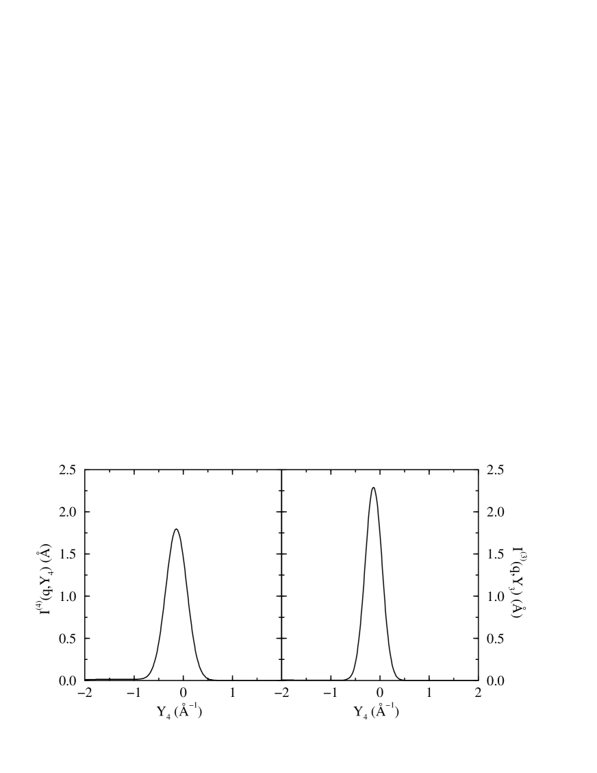
FIG. 9.: ⁴He (left) and ³He (right) instrumental resolution functions at $x=0.095$ and $q=23.1$ Å^-1.

FIG. 10.: Comparison of the theoretical generalized Compton profile (solid line) and the experimental measurements of Wang and Sokol[8] of the $x=0.095$ mixture at $q=23.1$ Å^-1 and $T=1.4$K (points with errorbars).

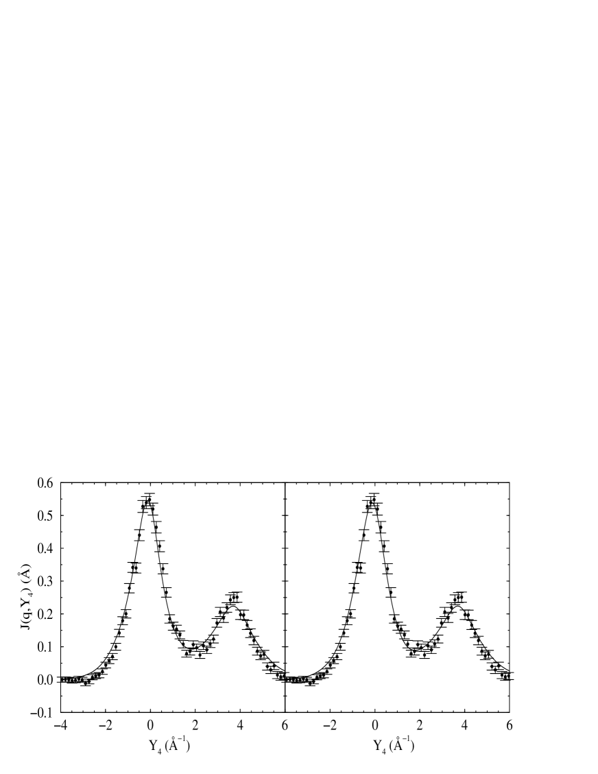
FIG. 11.: The $x=0.095$ experimental data of Wang and Sokol[8] compared to the response obtained from an alternative $\overline{\rho}_{1}^{(4)}(r)$ with $n_{0}=0.14$ and $\overline{t}_{4}=t_{4}=13.9$ K (solid line) –left panel–, and with $n_{0}=0.10$ and $\overline{t}_{4}=13.0$ K (solid line) –right panel–.