Critical behavior of the three-dimensional XY universality class

Abstract

We improve the theoretical estimates of the critical exponents for the three-dimensional XY universality class. We find $\alpha=-0.0146(8)$, $\gamma=1.3177(5)$, $\nu=0.67155(27)$, $\eta=0.0380(4)$, $\beta=0.3485(2)$, and $\delta=4.780(2)$. We observe a discrepancy with the most recent experimental estimate of $\alpha$; this discrepancy calls for further theoretical and experimental investigations. Our results are obtained by combining Monte Carlo simulations based on finite-size scaling methods, and high-temperature expansions. Two improved models (with suppressed leading scaling corrections) are selected by Monte Carlo computation. The critical exponents are computed from high-temperature expansions specialized to these improved models. By the same technique we determine the coefficients of the small-magnetization expansion of the equation of state. This expansion is extended analytically by means of approximate parametric representations, obtaining the equation of state in the whole critical region. We also determine the specific-heat amplitude ratio.

October 24, 2000

I Introduction

In the theory of critical phenomena continuous phase transitions can be classified into universality classes determined only by a few properties characterizing the system, such as the space dimensionality, the range of interaction, the number of components of the order parameter, and the symmetry. Renormalization-group (RG) theory predicts that, within a given universality class, critical exponents and scaling functions are identical for all systems. Here we consider the three-dimensional XY universality class, which is characterized by a two-component order parameter, ${\rm O}(2)$ symmetry, and short-range interactions.

The superfluid transition of ⁴He, whose order parameter is related to the complex quantum amplitude of the helium atoms, belongs to the three-dimensional XY universality class. It provides an exceptional opportunity for an experimental test of the RG predictions, essentially because of the weakness of the singularity in the compressibility of the fluid, of the purity of the samples, and of the possibility of performing the experiments, such as the Space Shuttle experiment reported in [1], in a microgravity environment, thereby reducing the gravity-induced broadening of the transition. Because of these favorable conditions, the specific heat of liquid helium was accurately measured to within a few nK from the $\lambda$ transition, i.e., very deep in the critical region, where the scaling corrections to the expected power-law behavior are small. The experimental low-temperature data for the specific heat were analyzed assuming the behavior for $t\equiv(T-T_{c})/T_{c}\to 0$

$$C_{H}(t)=A|t|^{-\alpha}\left(1+C|t|^{\Delta}+Dt\right)+B$$ (1)

with $\Delta=1/2$. This provided the estimate [1, 4]

$$\alpha=-0.01056(38).$$ (2)

This result represents a challenge for theorists because its uncertainty is substantially smaller than those of the theoretical calculations. We mention the best available theoretical estimates of $\alpha$: $\alpha=-0.0150(17)$ obtained using high-temperature (HT) expansion techniques [6], $\alpha=-0.0169(33)$ from Monte Carlo (MC) simulations using finite-size scaling (FSS) techniques [3], and $\alpha=-0.011(4)$ from field theory [2].

The aim of this paper is to substantially improve the precision of the theoretical estimates of the critical exponents, reaching an accuracy comparable with the experimental one. For this purpose, we will consider what we call “improved” models. They are characterized by the fact that the leading correction to scaling is absent in the expansion of any observable near the critical point. Moreover, we will combine MC simulations and analyses of HT series. We exploit the effectiveness of MC simulations to determine, by using FSS techniques, the critical temperature and the parameters of the improved Hamiltonians, and the effectiveness of HT methods to determine the critical exponents for improved models, especially when a precise estimate of $\beta_{c}$ is available. Such a combination of lattice techniques allows us to substantially improve earlier theoretical estimates. We indeed obtain

$$\alpha=-0.0146(8),$$ (3)

where, as we will show, the error estimate should be rather conservative. The theoretical uncertainty has been substantially reduced. We observe a disagreement with the experimental value (2). The point to be clarified is whether this disagreement is significant, or it is due to an underestimate of the errors reported by us and/or in the experimental papers. We think that this discrepancy calls for further theoretical and experimental investigations. A new-generation experiment in microgravity environment is currently in preparation [7]; it should clarify the issue from the experimental side.

In numerical (HT or MC) determinations of critical quantities, nonanalytic corrections to the leading scaling behavior represent one of the major sources of systematic errors. Considering, for instance, the magnetic susceptibility, we have

$$\chi=Ct^{-\gamma}\left(1+a_{0,1}t+a_{0,2}t^{2}+...+a_{1,1}t^{\Delta}+a_{1,2}t^{2\Delta}+...+a_{2,1}t^{\Delta_{2}}+...\right).$$ (4)

The leading exponent $\gamma$ and the correction-to-scaling exponents $\Delta,\Delta_{2},...$, are universal, while the amplitudes $C$ and $a_{i,j}$ are nonuniversal. For three-dimensional XY systems, the value of the leading correction-to-scaling exponent is $\Delta\approx 0.53$ [3, 2], and the value of the subleading exponent is $\Delta_{2}\approx 2\Delta$ [8].

The leading nonanalytic correction $t^{\Delta}$ is the dominant source of systematic errors in MC and HT studies. Indeed, in MC simulations the presence of this slowly-decreasing term requires careful extrapolations, increasing the errors in the final estimates. In HT studies, nonanalytic corrections introduce large and dangerously undetectable systematic deviations in the results of the analyses. Integral approximants [9] (see, e.g., Ref. [10] for a review) can in principle cope with an asymptotic behavior of the form (4); however, in practice, they are not very effective when applied to the series of moderate length available today. Analyses meant to effectively allow for the leading confluent corrections are based on biased approximants, where the value of $\beta_{c}$ and the first non-analytic exponent $\Delta$ are introduced as external inputs (see e.g. Refs. [11, 12, 13, 14, 15, 16]). Nonetheless, their precision is still not comparable to that of the experimental result (2), see e.g. Ref. [13]. The use of improved Hamiltonians, i.e., models for which the leading correction to scaling vanishes ($a_{1,1}=0$ in Eq. (4)), can lead to an additional improvement of the precision, even without a substantial extension of the HT series.

The use of improved Hamiltonians was first suggested in the early 80s by Chen, Fisher, and Nickel [17] who determined improved Hamiltonians in the Ising universality class. The crux of the method is a precise determination of the optimal value of the parameter appearing in the Hamiltonian. One can determine it from the analysis of HT series, but in this case it is obtained with a relatively large error [17, 18, 19, 20, 16] and the final results do not significantly improve the estimates obtained from standard analyses using biased approximants.

Recently [21, 22, 23, 24, 3, 16] it has been realized that FSS MC simulations are very effective in determining the optimal value of the parameter, obtaining precise estimates for several models in the Ising and XY universality classes. The same holds true of models in the ${\rm O}(3)$ and ${\rm O}(4)$ universality classes [25]. Correspondingly, the analysis of FSS results obtained in these simulations has provided significantly more precise estimates of critical exponents. An additional improvement of the precision of the results has been obtained by combining improved Hamiltonians and HT methods. Indeed, we already showed that the analysis of HT series for improved models [16, 6, 26] provides estimates that are substantially more precise than those obtained from the extrapolation of the MC data alone.

In this paper we consider again the XY case. The progress with respect to the studies of Refs. [6, 26] is essentially due to the improved knowledge of $\beta_{c}$ and of the parameters of the improved Hamiltonians obtained by means of a large-scale MC simulation. The use of this information in the analysis of the improved HT (IHT) series allows us to substantially increase the precision and the reliability of the results, especially of the critical exponents. As we shall see, in order to determine the critical exponents, the extrapolation to $\beta_{c}$ of the IHT series, using biased integral approximants, is more effective than the extrapolation $L\rightarrow\infty$ of the FSS MC data. Moreover, we consider two improved Hamiltonians. The comparison of the results from these two models provides a check of the errors we quote. The estimates obtained for the two models are in very good agreement, providing support for our error estimates and thus confirming our claim that the systematic error due to confluent singularities is largely reduced when analyzing IHT expansions.

We consider a simple cubic (sc) lattice, two-component vector fields $\vec{\phi}_{x}=(\phi_{x}^{(1)},\phi_{x}^{(2)})$, and two classes of models depending on an irrelevant parameter: the $\phi^{4}$ lattice model and the dynamically diluted XY (dd-XY) model.

The Hamiltonian of the $\phi^{4}$ lattice model is given by

$${\cal H}_{\phi^{4}}=-\beta\sum_{\left<xy\right>}{\vec{\phi}}_{x}\cdot{\vec{\phi}}_{y}+\,\sum_{x}\left[{\vec{\phi}}_{x}^{2}+\lambda({\vec{\phi}}_{x}^{2}-1)^{2}\right].$$ (5)

The dd-XY model is defined by the Hamiltonian

$${\cal H}_{\rm dd}=-\beta\sum_{\left<xy\right>}\vec{\phi}_{x}\cdot\vec{\phi}_{y}-D\sum_{x}\vec{\phi}_{x}^{2},$$ (6)

by the local measure

$$d\mu(\phi_{x})=\int d\phi_{x}^{(1)}\,\int d\phi_{x}^{(2)}\,\left[\delta(\phi_{x}^{(1)})\,\delta(\phi_{x}^{(2)})+\frac{1}{2\pi}\,\delta(1-|\vec{\phi}_{x}|)\right],$$ (7)

and the partition function

$$\int\prod_{x}d\mu(\phi_{x})\,e^{-{\cal H}_{\rm dd}}.$$ (8)

In the limit $D\rightarrow\infty$ the standard XY lattice model is recovered. We expect the phase transition to become of first order for $D<D_{\rm tri}$. $D_{\rm tri}$ vanishes in the mean-field approximation, while an improved mean-field calculation based on the “star approximation” of Ref. [27] gives $D_{\rm tri}<0$, so that we expect $D_{\rm tri}<0$.

The parameters $\lambda$ in ${\cal H}_{\phi^{4}}$ and $D$ in ${\cal H}_{\rm dd}$ can be tuned to obtain improved Hamiltonians. We performed an accurate numerical study, which provided estimates of $\lambda^{*}$, $D^{*}$, of the inverse critical temperature $\beta_{c}$ for several values of $\lambda$ and $D$, as well as estimates of the critical exponents. Using the linked-cluster expansion technique, we computed HT expansions of several quantities for the two theories. We analyzed them using the MC results for $\lambda^{*}$, $D^{*}$ and $\beta_{c}$, obtaining very accurate results, e.g., Eq. (3).

We mention that the $\phi^{4}$ lattice model ${\cal H}_{\phi^{4}}$ has already been considered in MC and HT studies [3, 6, 26]. With respect to those works, we have performed additional MC simulations to improve the estimate of $\lambda^{*}$ and determine the values of $\beta_{c}$. Moreover, we present a new analysis of the IHT series that uses the MC estimates of $\beta_{c}$ to bias the approximants, leading to a substantial improvement of the results.

In Table I we report our results for the critical exponents, i.e., our best estimates obtained by combining MC and IHT techniques—they are denoted by MC+IHT—together with the results obtained from the analysis of the MC data alone. There, we also compare them with the most precise experimental and theoretical estimates that have been obtained in the latest years. When only $\nu$ or $\alpha$ is reported, we used the hyperscaling relation $2-\alpha=3\nu$ to obtain the missing exponent. Analogously, if only $\eta$ or $\gamma$ is quoted, the second exponent was obtained using the scaling relation $\gamma=(2-\eta)\nu$; in this case the uncertainty was obtained using the independent-error formula. The results we quote have been obtained from the analysis of the HT series of the XY model (HT), by Monte Carlo simulations (MC) or by field-theory methods (FT). The HT results of Ref. [13] have been obtained analyzing the 21st-order HT expansions for the standard XY model on the sc and the bcc lattice, using biased approximants and taking $\beta_{c}$ and $\Delta$ from other approaches, such as MC and FT. The FT results of Refs. [2, 28] have been derived by resumming the known terms of the fixed-dimension $g$ expansion: the $\beta$ function is known to six-loop order [29], while the critical-exponent series are known to seven loops [30]. The estimates from the $\epsilon$ expansion have been obtained resumming the available $O(\epsilon^{5})$ series [31, 32].

TABLE I.: Estimates of the critical exponents. See text for the explanation of the symbols in the second column. We indicate with an asterisk (^∗) the estimates that have been obtained using the hyperscaling relation $2-\alpha=3\nu$ or the scaling relation $\gamma=(2-\eta)\nu$.

Ref.	Method	$\gamma$		$\nu$		$\eta$		$\alpha$
this work	MC+IHT	1	.3177(5)	0	.67155(27)	0	.0380(4)	$-$0	.0146(8)∗
this work	MC	1	.3177(10)∗	0	.6716(5)	0	.0380(5)	$-$0	.0148(15)∗
[6] (2000)	IHT	1	.3179(11)	0	.67166(55)	0	.0381(3)	$-$0	.0150(17)∗
[33] (1999)	HT							$-$0	.014(9), $-$0.022(6)
[13] (1997)	HT, sc	1	.325(3)	0	.675(2)	0	.037(7)∗	$-$0	.025(6)∗
	HT, bcc	1	.322(3)	0	.674(2)	0	.039(7)∗	$-$0	.022(6)∗
[3] (1999)	MC	1	.3190(24)∗	0	.6723(11)	0	.0381(4)	$-$0	.0169(33)∗
[34] (1999)	MC	1	.315(12)∗	0	.6693(58)	0	.035(5)	$-$0	.008(17)∗
[35] (1996)	MC	1	.316(3)∗	0	.6721(13)	0	.0424(25)	$-$0	.0163(39)∗
[36] (1995)	MC			0	.6724(17)			$-$0	.017(5)∗
[37] (1993)	MC	1	.307(14)∗	0	.662(7)	0	.026(6)	$-$0	.014(21)∗
[38] (1990)	MC	1	.316(5)	0	.670(2)	0	.036(14)∗	$-$0	.010(6)∗
[28] (1999)	FT $d=3$ exp	1	.3164(8)	0	.6704(7)	0	.0349(8)	$-$0	.0112(21)
[2] (1998)	FT $d=3$ exp	1	.3169(20)	0	.6703(15)	0	.0354(25)	$-$0	.011(4)
[2] (1998)	FT $\epsilon$-exp	1	.3110(70)	0	.6680(35)	0	.0380(50)	$-$0	.004(11)
[1, 4] (1996)	4He			0	.67019(13)∗			$-$0	.01056(38)
[39] (1993)	4He			0	.6705(6)			$-$0	.0115(18)∗
[40] (1992)	4He			0	.6708(4)			$-$0	.0124(12)∗
[41] (1984)	4He			0	.6717(4)			$-$0	.0151(12)∗
[42] (1983)	4He			0	.6709(9)∗			$-$0	.0127(26)

We also present a detailed study of the equation of state. We first consider its expansion in terms of the magnetization in the high-temperature phase. The coefficients of this expansion are directly related to the zero-momentum $n$-point renormalized couplings, which were determined by analyzing their IHT expansion. These results are used to construct parametric representations of the critical equation of state which are valid in the whole critical region, satisfy the correct analytic properties (Griffiths’ analyticity), and take into account the Goldstone singularities at the coexistence curve. From our approximate representations of the equation of state we derive estimates of several universal amplitude ratios. The specific-heat amplitude ratio is particularly interesting since it can be compared with experimental results. We obtain $A^{+}/A^{-}=1.062(4)$, which is not in agreement with the experimental result $A^{+}/A^{-}=1.0442$ of Refs. [1, 4]. It is easy to trace the origin of the discrepancy. In our method as well as in the analysis of the experimental data, the estimate of $A^{+}/A^{-}$ is strongly correlated with the estimate of $\alpha$. Therefore, the discrepancy we observe for this ratio is a direct consequence of the difference in the estimates of $\alpha$.

Finally, we also discuss the two-point function of the order parameter, i.e., the structure factor, which is relevant in scattering experiments with magnetic materials.

The paper is organized as follows. In Sec. II we present our Monte Carlo results. After reviewing the basic RG ideas behind our methods, we present a determination of the improved Hamiltonians and of the critical exponents. We discuss the several possible sources of systematic errors, and show that the approximate improved models we use have significantly smaller corrections than the standard XY model. A careful analysis shows that the leading scaling corrections are reduced at least by a factor of 20. We also compute $\beta_{c}$ to high precision for several values of $\lambda$ and $D$; this is an important ingredient in our IHT analyses. Details on the algorithm appear in App. A.

In Sec. III we present our results for the critical exponents obtained from the analysis of the IHT series. The equation of state is discussed in Sec. IV. After reviewing the basic definitions and properties, we present the coefficients of the small-magnetization expansion, again computed from IHT series. We discuss parametric representations that provide approximations of the equation of state in the whole critical region and compute several universal amplitude ratios. In Sec. V we analyze the two-point function of the order parameter. Details of the IHT analyses are reported in App. B. The definitions of the amplitude ratios we compute can be found in App. C.

II Monte Carlo Simulations

A The lattice and the quantities that were measured

We simulated sc lattices of size $V=L^{3}$, with periodic boundary conditions in all three directions. In addition to elementary quantities like the energy, the magnetization, the specific heat or the magnetic susceptibility we computed so-called phenomenological couplings, i.e., quantities that, in the critical limit, are invariant under RG transformations. They are well suited to locate the inverse critical temperature $\beta_{c}$. They also play a crucial role in the determination of the improved Hamiltonians.

In the present study we consider four phenomenological couplings. We use the Binder cumulant

$$U_{4}\equiv\frac{\langle(\vec{m}^{2})^{2}\rangle}{\langle\vec{m}^{2}\rangle^{2}},$$ (9)

and the analogous quantity with the 6th power of the magnetization

$$U_{6}\equiv\frac{\langle(\vec{m}^{2})^{3}\rangle}{\langle\vec{m}^{2}\rangle^{3}},$$ (10)

where $\vec{m}=\frac{1}{V}\,\sum_{x}\vec{\phi}_{x}$ is the magnetization of the system.

We also consider the second-moment correlation length divided by the linear extension of the lattice $\xi_{\rm 2nd}/L$. The second-moment correlation length is defined by

$$\xi_{\rm 2nd}\equiv\sqrt{\frac{\chi/F-1}{4\sin(\pi/L)^{2}}},$$ (11)

where

$$\chi\equiv\frac{1}{V}\left\langle\left(\sum_{x}\vec{\phi}_{x}\right)^{2}\right\rangle$$ (12)

is the magnetic susceptibility and

$$F\equiv\frac{1}{V}\left\langle\left|\sum_{x}\exp\left(i\frac{2\pi x_{1}}{L}\right)\vec{\phi}_{x}\right|^{2}\right\rangle$$ (13)

is the Fourier transform of the correlation function at the lowest non-zero momentum.

The list is completed by the ratio $Z_{a}/Z_{p}$ of the partition function $Z_{a}$ of a system with anti-periodic boundary conditions in one of the three directions and the partition function $Z_{p}$ of a system with periodic boundary conditions in all directions. Anti-periodic boundary conditions in the first direction are obtained by changing sign to the term $\vec{\phi}_{x}\vec{\phi}_{y}$ of the Hamiltonian for links $\left<xy\right>$ that connect the boundaries, i.e., for $x=(L,x_{2},x_{3})$ and $y=(1,x_{2},x_{3})$. The ratio $Z_{a}/Z_{p}$ can be measured by using the boundary-flip algorithm, which was applied to the three-dimensional Ising model in Ref. [43] and generalized to the XY model in Ref. [44]. As in Ref. [24], in the present work we used a version of the algorithm that avoids the flip to anti-periodic boundary conditions. For a detailed discussion see App. A 2.

B Summary of finite-size methods

In this subsection we discuss the FSS methods we used to compute the inverse critical temperature, the couplings $\lambda^{*}$ and $D^{*}$ at which leading corrections to scaling vanish, and the critical exponents $\nu$ and $\eta$.

1 Summary of basic RG results

The following discussion of FSS is based on the RG theory of critical phenomena. We first summarize some basic results. In the three-dimensional XY universality class there exist two relevant scaling fields $u_{t}$ and $u_{h}$, associated to the temperature and the applied field respectively, with RG exponents $y_{t}$ and $y_{h}$. Moreover, there are several irrelevant scaling fields that we denote by $u_{i}$, $i\geq 3$, with RG exponents $0>y_{3}>y_{4}>y_{5}>...\,$.

The RG exponent $y_{3}\equiv-\omega$ of the leading irrelevant scaling field $u_{3}$ has been computed by various methods. The analysis of field-theoretical perturbative expansions [2] gives $\omega=0.802(18)$ ($\epsilon$ expansion) and $\omega=0.789(11)$ ($d=3$ expansion). In the present work we find a result for $\omega$ that is consistent with, although less accurate than, the field-theoretical predictions. We also mention the estimate $\omega=0.85(7)$ that was obtained [8] by the “scaling-field” method, a particular implementation of Wilson’s “exact” renormalization group. Although it provides an estimate for $\omega$ that is less precise than those obtained from perturbative field-theoretic methods, it has the advantage of giving predictions for the irrelevant RG exponents beyond $y_{3}$. Ref. [8] predicts $y_{4}=-1.77(7)$ and $y_{5}=-1.79(7)$ ($y_{421}$ and $y_{422}$ in their notation) for the XY universality class. Note that, at present, there is no independent check of these results. Certainly it would be worthwhile to perform a Monte Carlo renormalization group study. With the computational power available today, it might be feasible to resolve subleading correction exponents with a high-statistics simulation.

In the case of $U_{4}$, $U_{6}$, and $\xi_{\rm 2nd}/L$ we expect a correction caused by the analytic background of the magnetic susceptibility. This should lead to corrections with $y_{6}=-(2-\eta)\approx-1.962$. We also expect corrections due to the violation of rotational invariance by the lattice. For the XY universality class, Ref. [45] predicts $y_{7}=-2.02(1)$. Note that the numerical values of $y_{6}$ and $y_{7}$ are virtually identical and should hence be indistinguishable in the analysis of our numerical data.

We wish now to discuss the FSS behavior of a phenomenological coupling $R$; in the standard RG framework, we can write it as a function of the thermal scaling field $u_{t}$ and of the irrelevant scaling fields $u_{i}$. For $L\to\infty$ and $\beta\to\beta_{c}(\lambda)$, we have

$$R(L,\beta,\lambda)=r_{0}(u_{t}L^{y_{t}})+\sum_{i\geq 3}r_{i}(u_{t}L^{y_{t}})\,u_{i}L^{y_{i}}+...\,,$$ (14)

where we have neglected terms that are quadratic in the scaling fields of the irrelevant operators, i.e., corrections of order $L^{2y_{3}}\approx L^{-1.6}$. Note that we include here the corrections due to the analytic background (with exponent $L^{-y_{6}}\approx L^{\eta-2}$). In the case of $U_{4}$, $U_{6}$, and $\xi_{\rm 2nd}/L$ (but not $Z_{a}/Z_{p}$), in Eq. (14) we have also discarded terms of order $L^{y_{t}-2y_{h}}\approx L^{-3.5}$.

The functions $r_{0}(z)$ and $r_{i}(z)$ are smooth and finite for $z\to 0$, while $u_{t}(\beta,\lambda)$ and $u_{i}(\beta,\lambda)$ are smooth functions of $\beta$ and $\lambda$. Note that, by definition, $u_{t}(\beta,\lambda)\sim\beta-\beta_{c}(\lambda)$. In the limit $t\to 0$ and $u_{t}L^{y_{t}}\sim(\beta-\beta_{c})L^{1/\nu}\to 0$, we can further expand Eq. (14), obtaining

$$R(L,\beta,\lambda)=R^{*}+c_{t}(\beta,\lambda)\,L^{y_{t}}+\sum_{i}c_{i}(\beta,\lambda)\,L^{y_{i}}+O((\beta-\beta_{c})^{2}L^{2y_{t}},L^{2y_{3}},tL^{y_{t}+y_{3}}),$$ (15)

where $R^{*}=r_{0}(0)$ is the value at the critical point of the phenomenological coupling.

2 Locating $\beta_{c}$

We locate the inverse critical temperature $\beta_{c}$ by using Binder’s cumulant crossing method. This method can be applied in conjunction with any of the four phenomenological couplings that we computed.

In its simplest version, one considers a phenomenological coupling $R(\beta,L)$ for two lattice sizes $L$ and $L^{\prime}=bL$. The intersection $\beta_{\rm cross}$ of the two curves $R(\beta,L)$ and $R(\beta,L^{\prime})$ provides an estimate of $\beta_{c}$. The convergence rate of this estimate $\beta_{\rm cross}$ towards the true value can be computed in the RG framework.

By definition, $\beta_{\rm cross}$ at fixed $b$, $L$, and $\lambda$ is given by the solution of the equation

$$R(L,\beta,\lambda)=R(bL,\beta,\lambda).$$ (16)

Using Eq. (14), one immediately verifies that $\beta_{\rm cross}$ converges to $\beta_{c}$ faster than $L^{-y_{t}}$. Thus, for $L\to\infty$, we can use Eq. (15) and rewrite Eq. (16) as

$$c_{t}(\beta,\lambda)\,L^{y_{t}}+c_{3}(\beta,\lambda)\,L^{y_{3}}\approx c_{t}(\beta,\lambda)\,(bL)^{y_{t}}+c_{3}(\beta,\lambda)\,(bL)^{y_{3}}.$$ (17)

Then, we approximate $c_{t}(\beta,\lambda)\approx c_{t}^{\prime}\,(\beta-\beta_{c})$ and $c_{i}(\beta,\lambda)\approx c_{i}(\beta_{c},\lambda)=c_{i}$. Remember that $c_{t}(\beta_{c},\lambda)=0$ by definition. Using these approximations we can explicitly solve Eq. (17) with respect to $\beta$, obtaining

$$\beta_{\rm cross}=\beta_{c}+\frac{c_{3}\,(1-b^{y_{3}})\,L^{y_{3}}}{c_{t}^{\prime}\,(b^{y_{t}}-1)\,L^{y_{t}}}+...\,.$$ (18)

The leading corrections vanish like $L^{-y_{t}+y_{3}}\approx L^{-2.3}$. Inserting $\beta_{\rm cross}$ into Eq. (16), we obtain

$$R_{\rm cross}=R^{*}+\frac{b^{y_{t}}-b^{y_{3}}}{b^{y_{t}}-1}\,L^{y_{3}}+...\,,$$ (19)

which shows that the leading corrections vanish like $L^{y_{3}}$.

Given a precise estimate of $R^{*}$, one can locate $\beta_{c}$ from simulations of a single lattice size, solving

$$R(L,\beta)=R^{*},$$ (20)

where the corrections vanish like $L^{-y_{t}+y_{3}}$.

3 Locating $\lambda^{*}$ and $D^{*}$

In order to compute the value $\lambda^{*}$ for which the leading corrections to scaling vanish, we use two phenomenological couplings $R_{1}$ and $R_{2}$. First, we define $\beta_{f}(L,\lambda)$ by

$$R_{1}(L,\beta_{f},\lambda)=R_{1,f}\,,$$ (21)

where $R_{1,f}$ is a fixed value, which we can choose freely within the appropriate range. It is easy to see that $\beta_{f}(L,\lambda)\to\beta_{c}(\lambda)$ as $L\to\infty$. Indeed, using Eq. (14), we have

$$\beta_{f}(L,\lambda)-\beta_{c}(\lambda)=z_{f}L^{-y_{t}}-{r_{1,3}(z_{f})\over r^{\prime}_{1,0}(z_{f})}u_{3}(\beta_{c})L^{y_{3}-y_{t}}+...\,,$$ (22)

where we have used $y_{t}>|y_{3}|$ and $z_{f}$ is defined as the solution of $r_{1,0}(z_{f})=R_{1,f}$. We have added a subscript 1 to make explicit that all scaling functions refer to $R_{1}$. If $R_{1,f}\approx R^{*}$, we can expand the previous formula, obtaining

$$\beta_{f}(L,\lambda)\approx\beta_{c}(\lambda)+{R_{1,f}-R_{1}^{*}\over{c_{1,t}^{\prime}}}L^{-y_{t}}-{c_{1,i}\over{c_{1,t}^{\prime}}}L^{-y_{t}+y_{3}}.$$ (23)

Notice that for $R_{1,f}=R_{1}^{*}$ the convergence is faster, and thus we will always take $R_{1,f}\approx R_{1}^{*}$. Next we define

$$\bar{R}(L,\lambda)\equiv R_{2}(L,\beta_{f},\lambda).$$ (24)

For $L\to\infty$ and $R_{1,f}\approx R^{*}_{1}$, we have

$$\bar{R}(L,\lambda) = R_{2}^{*}+\frac{c_{2,t}^{\prime}}{c_{1,t}^{\prime}}(R_{1,f}-R_{1}^{*})+\sum_{i}\left(c_{2,i}-\frac{c_{2,t}^{\prime}}{c_{1,t}^{\prime}}\,c_{1,i}\right)L^{y_{i}}$$ (25)

$$= \bar{R}^{*}+\sum_{i}\bar{c}_{i}(\lambda)\,L^{y_{i}},$$ (26)

which shows that the rate of convergence is determined by $L^{y_{3}}$.

In order to find $\lambda^{*}$, we need to compute the value of $\lambda$ for which $\bar{c}_{i}(\lambda)=0$. We can obtain approximate estimates of $\lambda^{*}$ by solving the equation

$$\bar{R}(L,\lambda)=\bar{R}(bL,\lambda).$$ (27)

Using the approximation (26) one finds

$$\lambda_{\rm cross}=\lambda^{*}-\frac{\bar{c}_{4}}{\bar{c}^{\,\prime}_{3}}\frac{1-b^{y}_{4}}{1-b^{y}_{3}}\,L^{y_{4}-y_{3}}+...\,,$$ (28)

where $\bar{c}^{\,\prime}_{3}$ is the derivative of $\bar{c}_{3}$ with respect to $\lambda$, and

$$\bar{R}_{\rm cross}=\bar{R}^{*}-\bar{c}_{4}\frac{b^{y}_{3}-b^{y}_{4}}{1-b^{y}_{3}}\,L^{y_{4}}.$$ (29)

In principle, any pair $R_{1}$, $R_{2}$ of phenomenological couplings can be used in this analysis. However, in practice we wish to see a good signal for the corrections. This means, in particular, that in $c_{1,t}^{\prime}\,c_{2,3}-c_{2,t}^{\prime}\,c_{1,3}$ the two terms should add up rather than cancel. Of course, also the corrections due to the subleading scaling fields should be small.

4 The critical exponents

Typically, the thermal RG exponent $y_{t}=1/\nu$ is computed from the FSS of the derivative of a phenomenological coupling $R$ with respect to $\beta$ at $\beta_{c}$. Using Eq. (14) one obtains

$$\left.\frac{\partial R}{\partial\beta}\right|_{\beta_{c}}=r_{0}^{\prime}(0)\,L^{y_{t}}+\sum_{i=3}r^{\prime}_{i}(0)\,u_{i}(\beta_{c})\,L^{y_{i}+y_{t}}+\sum_{i=3}r_{i}(0)\,u^{\prime}_{i}(\beta_{c})\,L^{y_{i}}+...\,.$$ (30)

Hence, the leading corrections scale with $L^{y_{3}}$. However, in improved models in which $u_{3}(\beta_{c})=0$, the leading correction is of order $L^{y_{4}}$. Note that corrections proportional to $L^{y_{3}-y_{t}}\approx L^{-2.3}$ are still present even if the model is improved. In Ref. [21], for the spin-1 Ising model, an effort was made to eliminate also this correction by taking the derivative with respect to an optimal linear combination of $\beta$ and $D$ instead of $\beta$. Here we make no attempt in this direction, since corrections of order $L^{-2.3}$ are subleading with respect to those of order $L^{y_{4}}\approx L^{-1.8}$.

In practice it is difficult to compute the derivative at $\beta_{c}$, since $\beta_{c}$ is only known numerically, and therefore, it is more convenient to evaluate $\partial R/\partial\beta$ at $\beta_{f}$ (see Eq. (21)). This procedure has been used before, e.g., in Ref. [35]. In this case, Eq. (30) still holds, although with different amplitudes that depend on the particular choice of the value of $R_{f}$.

The exponent $\eta$ is computed from the finite-size behavior of the magnetic susceptibility, i.e.,

$$\left.\chi\right|_{\beta_{f}}\propto L^{2-\eta}.$$ (31)

Also here the corrections are of order $L^{y_{3}}$ for generic models, and of order $L^{y_{4}}$ for improved ones.

5 Estimating errors caused by residual leading scaling corrections

In Ref. [23], the authors pointed out that with the method discussed in Sec. II B 3, the leading corrections are only approximately eliminated, so that there is still a small leading scaling correction which causes a systematic error in the estimates of, e.g., the critical exponents. The most naive solution to this problem consists in adding a term $L^{-\omega}$ to the fit ansatz, i.e., in considering

$$\left.\frac{\partial R}{\partial\beta}\right|_{\beta_{f}}=A\,L^{1/\nu}\left(1+B\,L^{-\omega}\right).$$ (32)

However, by adding such a correction term, the precision of the result decreases, so that there is little advantage in using (approximately) improved models. A more sophisticated approach is based on the fact that ratios of leading correction amplitudes are universal [46].

Let us consider a second phenomenological coupling $\bar{R}=R(L,\beta_{f},\lambda)$, which, for $L\to\infty$, behaves as

$$\bar{R}=\bar{R}^{*}+\bar{c}_{3}\,L^{-\omega}.$$ (33)

The universality of the correction amplitudes implies that the ratio $B/\bar{c}_{3}$ is the same for the $\phi^{4}$ model and the dd-XY model and is independent of $\lambda$ and $D$. Therefore, this ratio can be computed in models that have large corrections to scaling, e.g., in the standard XY model. Then, we can compute a bound on $B$ for the (approximately) improved model from the known ratio $B/\bar{c}_{3}$ and a bound for $\bar{c}_{3}$. This procedure was proposed in Ref. [21].

C The simulations

We simulated the $\phi^{4}$ and the dd-XY model using the wall-cluster update algorithm of Ref. [21] combined with a local update scheme. The update algorithm is discussed in detail in App. A, where we also report an analysis of its performance and the checks we have done.

Most of the analyses need the quantities as functions of $\beta$. Given the large statistics, we could not store all individual measurements of the observables. Therefore, we did not use the reweighting method. Instead, we determined the Taylor coefficients of all quantities of interest up to the third order in $(\beta-\beta_{s})$, where $\beta_{s}$ is the value of $\beta$ at which the simulation was performed. We checked carefully that this is sufficient for our purpose. For details, see App. A.

Most of our simulations were performed at $\lambda=2.1$ in the case of the $\phi^{4}$ model and at $D=1.03$ in the case of the dd-XY model. $\lambda=2.1$ is the estimate of $\lambda^{*}$ of Ref. [3], and $D=1.03$ is the result for $D^{*}$ of a preliminary analysis of MC data obtained on small lattices.

In addition, we performed simulations at $\lambda=2.0$ and $2.2$ for the $\phi^{4}$ model and $D=0.9$ and $1.2$ for the dd-XY model in order to obtain an estimate of the derivative of the amplitude of the leading corrections to scaling with respect to $\lambda$ and $D$, respectively.

We also performed simulations of the standard XY model in order to estimate the effect of the leading corrections to scaling on the estimates of the critical exponents obtained from the FSS analysis.

D $\beta_{c}$ and the critical value of phenomenological couplings

In a first step of the analysis we computed $R^{*}$ and the inverse critical temperature $\beta_{c}$ at $\lambda=2.1$ and $D=1.03$ respectively.

For $\lambda=2.1$ and $D=1.03$ we simulated sc lattices of linear size $L$ from $4$ to $16$ and $L=18$, $20$, $22$, $24$, $26$, $28$, $32$, $36$, $40$, $48$, $56$, $64$, and $80$. For all lattice sizes smaller than $L=24$ we performed $10^{8}$ measurements, except for the dd-XY model at $L=16$ where approximately $1.5\times 10^{8}$ measurements were performed. The statistics for the larger lattices is given in Table II. A measurement was performed after an update cycle as discussed in App. A 1.

TABLE II.: The number of measurements/1000 for the $\phi^{4}$ model at $\lambda=2.1$ and for the dd-XY model at $D=1.03$ for linear lattice sizes $L\geq 24$.

$L$	$\phi^{4}$	dd-XY
24	100,000	112,740
26	28,475	60,900
28	101,235	80,645
32	48,005	55,560
36	18,220	22,880
40	21,120	27,115
48	9,735	16,005
56	6,550	7,495
64	4,725	5,240
80	585	780

Instead of computing $R^{*}$ and $\beta_{c}$ from two lattice sizes as discussed in Sec. II B 2, we perform a fit with the ansatz

$$R^{*}=R(L,\beta_{c}),$$ (34)

where $R^{*}$ and $\beta_{c}$ are free parameters. We compute $R(L,\beta)$ using its third-order Taylor expansion

$$R^{*}=R(L,\beta_{s})+d_{1}(L,\beta_{s})(\beta_{c}-\beta_{s})+\frac{1}{2}\,d_{2}(L,\beta_{s})(\beta_{c}-\beta_{s})^{2}+\frac{1}{6}\,d_{3}(L,\beta_{s})(\beta_{c}-\beta_{s})^{3},$$ (35)

where $\beta_{s}$ is the $\beta$ at which the simulation was performed, and $R$, $d_{1}$, $d_{2}$, and $d_{3}$ are determined in the MC simulation.

First, we perform fits for the two models separately. We obtain consistent results for $R^{*}$ for all four choices of phenomenological couplings. In order to obtain more precise results for $\beta_{c}$ and $R^{*}$, we perform joint fits of both models. Here, we exploit universality by requiring that $R^{*}$ takes the same value in both models. Hence, such fits have three free parameters: $R^{*}$ and the two values of $\beta_{c}$. In the following we shall only report the results of such joint fits.

Let us discuss in some detail the results for $R=Z_{a}/Z_{p}$ that are summarized in Table III. In each fit, we take all data with $L_{\rm min}\leq L\leq L_{\rm max}$ into account. For $L_{\rm max}=80$, the $\chi^{2}/$d.o.f. becomes approximately one starting from $L_{\rm min}=15$. However, we should note that a $\chi^{2}/$d.o.f. close to one does not imply that the systematic errors due to corrections that are not taken into account in the ansatz are negligible.

Our final result is obtained from the fit with $L_{\rm min}=28$ and $L_{\rm max}=80$. The systematic error is estimated by comparing this result with that obtained using $L_{\rm min}=10$ and $L_{\rm max}=28$. The systematic error on $\beta_{c}$ is estimated by the difference of the results from the two fits divided by $2.8^{2.3}-1$, where $2.8$ is the scale factor between the two intervals and $y_{t}-y_{3}\approx 2.3$. Estimating the systematic error by comparison with the interval $L_{\rm min}=14$ and $L_{\rm max}=40$ leads to a similar result. We obtain $\beta_{c}=0.5091507(6)[7]$ for the $\phi^{4}$ model at $\lambda=2.1$ and $\beta_{c}=0.5627975(7)[7]$ for the dd-XY model at $D=1.03$. In parentheses we give the statistical error and in the brackets the systematic one. Our final result for the critical ratio of partition functions is $(Z_{a}/Z_{p})^{*}=0.3202(1)[5]$. Here the systematic error is computed by dividing the difference of the results of the two fits by $2.8^{0.8}-1$.

TABLE III.: Joint fits of the $Z_{a}/Z_{p}$ data of the $\phi^{4}$ model and the dd-XY model with the ansatz (35). All lattice sizes $L_{\rm min}\leq L\leq L_{\rm max}$ are used in the fit. In column four we give the results of the fits for $\beta_{c}$ of the $\phi^{4}$ model at $\lambda=2.1$ and in column five the results for $\beta_{c}$ of the dd-XY model at $D=1.03$. Finally, in column six we give the results for the fixed-point value $(Z_{a}/Z_{p})^{*}$. The final results and an estimate of the systematic errors are given in the text.

$L_{\rm min}$	$L_{\rm max}$	$\chi^{2}$/d.o.f.	$\beta_{c}$, $\lambda=2.1$	$\beta_{c}$, $D=1.03$	$(Z_{a}/Z_{p})^{*}$
11	80	3.25	0.50915354(33)	0.56280014(35)	0.319794(25)
13	80	2.48	0.50915287(35)	0.56279938(38)	0.319883(29)
15	80	1.06	0.50915192(38)	0.56279834(41)	0.320019(35)
20	80	0.91	0.50915142(46)	0.56279784(49)	0.320093(52)
24	80	0.89	0.50915109(53)	0.56279740(56)	0.320162(72)
28	80	0.73	0.50915074(63)	0.56279747(66)	0.320195(102)
32	80	0.85	0.50915065(75)	0.56279746(82)	0.320208(149)
10	28	3.47	0.50915783(53)	0.56280463(59)	0.319524(32)
14	40	1.78	0.50915337(48)	0.56279981(53)	0.319877(39)

We repeat this analysis for $\xi_{\rm 2nd}$, $U_{4}$ and $U_{6}$. The final results are summarized in Table IV.

TABLE IV.: Summary of the final results for $\beta_{c}$ and $R^{*}$. In column one the choice of the phenomenological coupling $R$ is listed. In columns two and three we report our estimates of $\beta_{c}$ for the $\phi^{4}$ model at $\lambda=2.1$ and the dd-XY model at $D=1.03$, and finally in column four the result for the fixed-point value of the phenomenological coupling. Note that the estimates of $\beta_{c}$, based on the four different choices of $R$, are consistent within error bars.

$R$	$\beta_{c}$, $\lambda=2.1$	$\beta_{c}$, $D=1.03$	$R^{*}$
$Z_{a}/Z_{p}$	0.5091507(6)[7]	0.5627975(7)[7]	0.3202(1)[5]
$\xi_{\rm 2nd}/L$	0.5091507(7)[3]	0.5627971(7)[2]	0.5925(1)[2]
$U_{4}$	0.5091495(9)[10]	0.5627972(10)[11]	1.2430(1)[5]
$U_{6}$	0.5091498(9)[15]	0.5627976(10)[15]	1.7505(3)[25]

Next we compute $\beta_{c}$ at additional values of $\lambda$ and $D$. For this purpose we simulated lattices of size $L=96$ and compute $\beta_{c}$ using Eq. (20). We use only $R=Z_{a}/Z_{p}$ with the above-reported estimate $(Z_{a}/Z_{p})^{*}=0.3202(6)$. The results are summarized in Table V.

TABLE V.: Estimates of $\beta_{c}$ from simulations of $96^{3}$ lattices. $\beta_{c}$ is obtained from Eq. (20) using $Z_{a}/Z_{p}$ as phenomenological coupling. In parentheses we give the statistical error and in brackets the error due to the error on $(Z_{a}/Z_{p})^{*}$. “stat” gives (the number of measurements)/1000.

model	$\lambda$ ; $D$	stat	$\beta_{c}$
$\phi^{4}$	2.07	545	0.5093853(16)[8]
$\phi^{4}$	2.2	510	0.5083366(16)[8]
dd-XY	0.9	720	0.5764582(15)[9]
dd-XY	1.02	1,215	0.5637972(12)[9]
dd-XY	1.2	665	0.5470377(17)[9]

E Eliminating leading corrections to scaling

In this subsection we determine $\lambda^{*}$ and $D^{*}$. For this purpose, we compute the correction amplitude $\bar{c}_{3}$ for various choices of $R_{1}$ and $R_{2}$ for the $\phi^{4}$ model at $\lambda=2.1$ and the dd-XY model at $D=1.03$. In order to convert these results into estimates of $\lambda^{*}$ and $D^{*}$, we determine the derivative of the correction amplitude $\bar{c}_{3}$ with respect to $\lambda$ (resp. $D$) at $\lambda=2.1$ (resp. $D=1.03$). We also simulated the XY model in order to obtain estimates of the residual systematic error due to the leading corrections to scaling. Note that, in the following, we always use as the value of $R_{1,f}$ in Eq. (21) the estimates of $R^{*}$ given in Table IV.

1 Derivative of the correction amplitude with respect to $\lambda$ or $D$

For this purpose we simulated the dd-XY model at $D=0.9$ and $D=1.2$ on lattices of size $L=5$, $6$, $7$, $8$, $9$, $10$, $12$ and $16$. The $\phi^{4}$ model was simulated at $\lambda=2.0$ and $\lambda=2.2$ on lattices of size $L=3$, $4$, $5$, $6$, $7$, $8$ and $9$. In the case of the dd-XY model we performed $100\times 10^{6}$ measurements for each parameter set. In the case of the $\phi^{4}$ model $250\times 10^{6}$ measurements were performed.

In the following we discuss only the dd-XY model, since the analysis of the $\phi^{4}$ data is performed analogously.

In Refs. [24, 3] it was observed that subleading corrections to scaling cancel to a large extent when one considers the difference of $\bar{R}$ at close-by values of $\lambda$. In order to get an idea of the size of the corrections, we report in Table VI

$$\Delta\bar{R}\,L^{0.8}=(\bar{R}|_{D=0.9}-\bar{R}|_{D=1.2})\,L^{0.8}$$ (36)

for various choices of $R_{1}$ and $R_{2}$. We see that this quantity varies little with $L$ in all cases. In the case of $R_{1}=Z_{a}/Z_{p}$ and $R_{2}=U_{4}$, $\Delta\bar{R}\,L^{0.8}$ is already constant within error bars starting from $L=5$.

In order to compute $\overline{c}_{3}$, see Eq. (26), we need $\Delta\bar{R}\,L^{0.8}$ to be as flat as possible and especially $\Delta\bar{R}$ large compared to the statistical errors. Looking at Table VI, we see that the two combinations $R_{1}=\xi_{\rm 2nd}/L$, $R_{2}=Z_{a}/Z_{p}$ and $R_{1}=U_{4}$, $R_{2}=U_{6}$ are unfavorable compared with the other four combinations.

TABLE VI.: The quantity $(\bar{R}|_{D=0.9}-\bar{R}|_{D=1.2})L^{0.8}$ for the dd-XY model. In the top row we give the choice of $R_{1}$ and $R_{2}$. For instance, $U_{4}$ at $(Z_{a}/Z_{p})_{f}$ means that $R_{1}=Z_{a}/Z_{p}$ and $R_{2}=U_{4}$.

$L$	$U_{4}$ at $(Z_{a}/Z_{p})_{f}$	$U_{6}$ at $(Z_{a}/Z_{p})_{f}$	$U_{4}$ at $(\xi_{\rm 2nd}/L)_{f}$	$U_{6}$ at $(\xi_{\rm 2nd}/L)_{f}$	$Z_{a}/Z_{p}$ at $(\xi_{\rm 2nd}/L)_{f}$	$U_{6}$ at $U_{4,f}$
5	0.0366(2)	0.1294(7)	0.0400(2)	0.1404(7)	0.0057(2)	0.0039(1)
6	0.0365(2)	0.1297(8)	0.0409(3)	0.1442(9)	0.0069(2)	0.0042(1)
7	0.0368(3)	0.1312(9)	0.0415(3)	0.1469(10)	0.0073(3)	0.0046(2)
8	0.0369(3)	0.1312(10)	0.0421(3)	0.1489(11)	0.0081(3)	0.0046(2)
9	0.0366(4)	0.1301(12)	0.0415(3)	0.1468(13)	0.0076(3)	0.0044(2)
10	0.0368(4)	0.1311(13)	0.0419(4)	0.1483(14)	0.0078(4)	0.0045(2)
12	0.0372(4)	0.1324(15)	0.0427(5)	0.1511(17)	0.0084(4)	0.0045(3)
16	0.0360(6)	0.1286(20)	0.0411(7)	0.1460(22)	0.0078(5)	0.0046(4)

In order to see whether we can predict the exponent $\omega$, we perform a fit with the ansatz

$$\Delta\bar{R}=k\,L^{-\omega},$$ (37)

with $k$ and $\omega$ as free parameters. From $U_{4}$ at $Z_{a}/Z_{p}=0.3202$ we get $\omega=0.795(9)$ with $\chi^{2}/\mbox{d.o.f.}=0.66$, using all available data. This value is certainly consistent with field-theoretical results. Note however, that we would like to vary the range of the fit in order to estimate systematic errors. For this purpose more data at larger values of $L$ are needed.

In the following we need estimates of

$$\left.\frac{d\bar{c}_{3}}{dD}\right|_{D=1.03}$$ (38)

and of the corresponding quantity for the $\phi^{4}$ model, in order to determine $D^{*}$ and $\lambda^{*}$. We approximated this derivative by a finite difference between $D=0.9$ and $D=1.2$. The coefficient $\bar{c}_{3}$ is determined by fixing $\omega=0.8$. Our final result is the average of the estimates for $L=10,12$ and 16 in Table VI. In a similar way we proceed in the case of the $\phi^{4}$ model, averaging the $L=8,9$ results. The results are summarized in Table VII. We make no attempt to estimate error bars. Sources of error are the finite difference in $D$, subleading corrections, the error on $\omega$ and the statistical errors. Note however that these errors are small enough to be neglected in the following.

TABLE VII.: Estimates for $d\bar{c}_{3}/dD$ at $D=1.03$ (dd-XY) and $d\bar{c}_{3}/d\lambda$ at $\lambda=2.1$ ($\phi^{4}$). In the first row we give the combination of $R_{1}$ and $R_{2}$.

Model	$U_{4}$ at $(Z_{a}/Z_{p})_{f}$	$U_{6}$ at $(Z_{a}/Z_{p})_{f}$	$U_{4}$ at $(\xi_{\rm 2nd}/L)_{f}$	$U_{6}$ at $(\xi_{\rm 2nd}/L)_{f}$
dd-XY	$-$0.122	$-$0.435	$-$0.140	$-$0.495
$\phi^{4}$	$-$0.0490	$-$0.175	$-$0.0546	$-$0.194

2 Finding $\bar{R}^{*}$, $\lambda^{*}$ and $D^{*}$

For this purpose we fit our results at $D=1.03$ and $\lambda=2.1$ with the ansatz

$$\bar{R}=\bar{R}^{*}+\bar{c}_{3}\,L^{-\omega},$$ (39)

where we fix $\omega=0.8$. We convinced ourselves that setting $\omega$ = $0.75$ or $0.85$ changes the final results very little compared with statistical errors and errors caused by subleading corrections. We perform joint fits, by requiring $\bar{R}^{*}$ to be equal in both models.

The results of the fits for four different combinations of $R_{1}$ and $R_{2}$ are given in Table VIII, where we have already translated the results for $\bar{c}_{3}$ into an estimate of $\lambda^{*}$ and $D^{*}$, by using

$$\lambda^{*}=2.1-\bar{c}_{3}\left(\frac{d\bar{c}_{3}}{d\lambda}\right)^{-1}$$ (40)

for the $\phi^{4}$ model and the analogous formula for the dd-XY model, and the results of Table VII.

TABLE VIII.: Results of fits with the ansatz (39). The coefficients $\bar{c}_{3}$ are converted into $D^{*}$ and $\lambda^{*}$ using Eq. (40). All data with $L_{\rm min}\leq L\leq L_{\rm max}$ are fitted.

$L_{\rm min}$	$L_{\rm max}$	$\chi^{2}$/d.o.f.	$\bar{R}^{*}$	$\lambda^{*}$	$D^{*}$
$R_{1,f}=(Z_{a}/Z_{p})_{f}=0.3202$ and $R_{2}=U_{4}$.
8	80	1.55	1.24303(2)	2.077(4)	1.020(2)
12	80	1.01	1.24304(4)	2.071(8)	1.022(3)
16	80	1.07	1.24308(6)	2.057(14)	1.019(5)
20	80	1.12	1.24301(8)	2.073(22)	1.028(9)
8	40	1.62	1.24304(3)	2.077(4)	1.020(2)
10	40	1.02	1.24305(3)	2.070(6)	1.020(2)
$R_{1,f}=(Z_{a}/Z_{p})_{f}=0.3202$ and $R_{2}=U_{6}$.
8	80	2.15	1.75156(8)	2.006(4)	0.990(2)
12	80	1.15	1.75126(13)	2.018(7)	1.000(3)
16	80	1.22	1.75120(19)	2.017(13)	1.003(5)
20	80	1.19	1.75085(27)	2.043(21)	1.015(8)
8	40	2.21	1.75160(9)	2.004(4)	0.989(2)
10	40	1.24	1.75143(11)	2.010(6)	0.994(2)
$R_{1,f}=(\xi_{\rm 2nd}/L)_{f}=0.5925$ and $R_{2}=U_{4}$.
8	80	4.01	1.24352(3)	1.977(4)	0.987(2)
12	80	1.19	1.24322(4)	2.031(8)	1.010(3)
16	80	1.29	1.24314(6)	2.049(14)	1.019(5)
20	80	1.13	1.24299(9)	2.083(23)	1.035(9)
8	40	4.19	1.24355(3)	1.973(4)	0.985(2)
10	40	1.49	1.24335(4)	2.006(6)	1.000(2)
$R_{1,f}=(\xi_{\rm 2nd}/L)_{f}=0.5925$ and $R_{2}=U_{6}$.
8	80	6.62	1.75323(10)	1.915(4)	0.961(2)
12	80	1.55	1.75189(14)	1.985(7)	0.991(3)
16	80	1.51	1.75142(22)	2.013(13)	1.004(5)
20	80	1.24	1.75078(32)	2.055(22)	1.024(8)
8	40	7.02	1.75336(10)	1.911(4)	0.959(2)
10	40	2.21	1.75248(12)	1.953(6)	0.978(2)

A $\chi^{2}$/d.o.f. close to $1$ is reached for $L_{\rm min}=10$ and $L_{\rm max}=80$ in the case of $U_{4}$ at $(Z_{a}/Z_{p})_{f}=0.3202$. This has to be compared with $L_{\rm min}=11$, $11$, and $14$ in the case of $U_{6}$ at $(Z_{a}/Z_{p})_{f}=0.3202$, $U_{4}$ at $(\xi_{\rm 2nd}/L)_{f}=0.5925$ and $U_{6}$ at $(\xi_{\rm 2nd}/L)_{f}=0.5925$.

This indicates that $U_{4}$ at $(Z_{a}/Z_{p})_{f}=0.3202$ has the least bias due to subleading corrections to scaling. Therefore we take as our final result $\lambda^{*}=2.07$ and $D^{*}=1.02$ which is the result of $L_{\rm min}=12$ and $L_{\rm max}=80$ in Table VIII. Starting from $L_{\rm min}=20$ all results for $\lambda^{*}$ and $D^{*}$ are within $2\sigma$ of our final result quoted above.

Our final results are $\lambda^{*}=2.07(5)$ and $D^{*}=1.02(3)$. The error bars are such to include all results in Table VIII with $L_{\rm min}=20$ and $L_{\rm max}=80$, including the statistical error, and therefore should take into proper account all systematic errors.

From these results, it is also possible to obtain a conservative upper bound on the coefficient $\bar{c}_{3}$ for $\lambda=2.1$ and $D=1.03$. Indeed, using the estimates of $\lambda^{*}$ and $D^{*}$ and their errors, we can obtain the upper bounds $|2.1-\lambda^{*}|<\Delta\lambda=0.08$ and $|1.03-D^{*}|<\Delta D=0.04$. Then, we can estimate $|\bar{c}_{3}(\lambda=2.1)|<\Delta\lambda(d\bar{c}_{3}/d\lambda)$, and analogously $|\bar{c}_{3}(D=1.03)|<\Delta D(d\bar{c}_{3}/dD)$. For $U_{4}$ at $(Z_{a}/Z_{p})_{f}=0.3202$, using the results of Table VII, we have

$$|\bar{c}_{3}(\lambda=2.1)|<0.004,\qquad\qquad|\bar{c}_{3}(D=1.03)|<0.005.$$ (41)

3 Corrections to scaling in the standard XY model

We simulated the standard XY model on lattices with linear sizes $L=6$, $8$, $10$, $12$, $16$, $18$, $20$, $22$, $24$, $28$, $32$, $48$, $56$, and $64$ at $\beta_{s}=0.454165$, which is the estimate of $\beta_{c}$ of Ref. [35]. Here, we used only the wall-cluster algorithm for the update. In one cycle we performed 12 wall-cluster updates. For $L\leq 16$ we performed $10^{8}$ cycles. For lattice sizes $16\leq L\leq 64$, we spent roughly the same amount of CPU time for each lattice size. For $L=64$ the statistics is $2.73\times 10^{6}$ measurements.

We determine the amplitude of the corrections to scaling for $\bar{R}$ with $R_{1,f}=(Z_{a}/Z_{p})_{f}=0.3202$ and $R_{2}=U_{4}$. Other choices lead to similar results. We fit our numerical results with the ansatz (39), where we fix $\omega=0.8$. The results are given in Table IX.

TABLE IX.: Corrections to scaling in the standard XY model for $\bar{R}$ with $R_{2}=U_{4}$ and $R_{1,f}=(Z_{a}/Z_{p})_{f}=0.3202$. We use the ansatz (39) with $\omega=0.8$ fixed.

$L_{\rm min}$	$L_{\rm max}$	$\chi^{2}$/d.o.f.	$\bar{R}^{*}$	$\bar{c}_{3}$
12	64	1.78	1.2432(1)	$-$0.1120(7)0
16	64	0.73	1.2430(1)	$-$0.1087(13)
20	64	0.38	1.2427(2)	$-$0.1048(22)
24	64	0.24	1.2429(2)	$-$0.1083(34)
12	32	2.32	1.2433(1)	$-$0.1124(8)0

Note that the results for $\bar{R}^{*}$ are consistent with the result obtained from the joint fit of the two improved models. In Table VIII we obtained, e.g., $\bar{R}^{*}=1.24301(8)$ with $L_{\rm min}=20$ and $L_{\rm max}=80$.

Corrections to scaling are clearly visible, see Fig. 1. From the fit with $L_{\rm min}=20$ and $L_{\rm max}=64$ we obtain $\bar{c}_{3}=-0.1048(22)$. For the following discussion no estimate of the possible systematic errors of $\bar{c}_{3}$ is needed. Comparing with Eq. (41), we see that in the (approximately) improved models the amplitude of the leading correction to scaling is at least reduced by a factor of 20. Note, that even if this result was obtained by considering a specific observable, $U_{4}$ at fixed $Z_{a}/Z_{p}$, the universality of the ratios of the subleading corrections implies the same reduction for any quantity. In the following section we will use this result to estimate the systematic error on our results for the critical exponents.

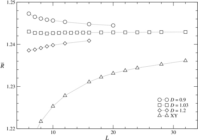
FIG. 1.: Corrections to scaling for the dd-XY model at $D=0.9$, $1.03$, and $1.2$, and for the standard XY model. We plot $\bar{R}$ with $R_{1,f}=(Z_{a}/Z_{p})_{f}=0.3202$ and $R_{2}=U_{4}$ as a function of the lattice size. The dotted lines should only guide the eye.

F Critical exponents from finite-size scaling

As discussed in Sec. II B, we may use the derivative of phenomenological couplings taken at $\beta_{f}$ in order to determine $y_{t}$. Given the four phenomenological couplings that we have implemented, this amounts to 16 possible combinations. In the following we will restrict the discussion to two choices: in both cases we fix $\beta_{f}$ by $(Z_{a}/Z_{p})_{f}=0.3202$. At $\beta_{f}$ we consider the derivative of the Binder cumulant and the derivative of $Z_{a}/Z_{p}$. In Table X we summarize the results of the fits with the ansatz

$$\left.\frac{\partial R}{\partial\beta}\right|_{\beta_{f}}=cL^{1/\nu}$$ (42)

for the $\phi^{4}$ model at $\lambda=2.1$, the dd-XY model at $D=1.03$, and the standard XY model.

TABLE X.: Fit results for the critical exponent $\nu$ obtained from the ansatz (42). In all cases $\beta_{f}$ is fixed by $Z_{a}/Z_{p,f}=0.3202$. We analyze the $\phi^{4}$ model at $\lambda=2.1$, the dd-XY model at $D=1.03$, and the standard XY model. We consider the slope of the Binder cumulant $U_{4}$ and of the ratio of partition functions $Z_{a}/Z_{p}$. We included all data with $L_{\rm min}\leq L\leq L_{\rm max}$ into the fit.

$L_{\rm min}$	$L_{\rm max}$	$\chi^{2}/$d.o.f.	$\nu$
$\phi^{4}$ model: derivative of $U_{4}$
07	80	1.17	0.67168(12)
09	80	0.79	0.67188(15)
11	80	0.85	0.67181(19)
16	80	0.98	0.67192(34)
$\phi^{4}$ model: derivative of $Z_{a}/Z_{p}$
12	80	3.01	0.67042(9)
16	80	1.61	0.67104(15)
20	80	1.04	0.67139(22)
24	80	0.54	0.67194(32)
dd-XY model: derivative of $U_{4}$
07	80	2.06	0.67258(12)
09	80	1.13	0.67216(15)
11	80	1.19	0.67209(19)
16	80	0.97	0.67154(31)
dd-XY model: derivative of $Z_{a}/Z_{p}$
12	80	1.89	0.67017(9)
16	80	1.60	0.67046(14)
20	80	0.79	0.67099(21)
24	80	0.80	0.67113(30)
XY model: derivative of $U_{4}$
12	64	4.48	0.66450(28)
16	64	1.30	0.66618(42)
20	64	0.54	0.66740(63)
XY model: derivative of $Z_{a}/Z_{p}$
12	64	1.33	0.67263(13)
16	64	0.69	0.67300(19)
20	64	0.30	0.67325(30)
24	64	0.25	0.67327(41)

We see that for the same $L_{\rm min}$ and $L_{\rm max}$ the statistical error on the estimate of $\nu$ obtained from the derivative of $Z_{a}/Z_{p}$ is smaller than that obtained from the derivative of $U_{4}$. On the other hand, for the two improved models, scaling corrections seem to be larger for $Z_{a}/Z_{p}$ than for $U_{4}$.

In the case of $Z_{a}/Z_{p}$, for both improved models, the result of the fit for $\nu$ is increasing with increasing $L_{\rm min}$. In the case of the Binder cumulant, it is increasing with $L_{\rm min}$ for the $\phi^{4}$ model and decreasing for the dd-XY model. The fact that scaling corrections affect the two quantities and the two improved models in a quite different way suggests that systematic errors in the estimate of $\nu$ can be estimated from the variation of the fits presented in Table X.

As our final result we quote $\nu=0.6716(5)$ which is consistent with the two results from $Z_{a}/Z_{p}$ at $L_{\rm min}=24$ and with the results from $U_{4}$ at $L_{\rm min}=16$.

In the case of the standard XY model, the derivative of $U_{4}$ requires a much larger $L_{\rm min}$ to reach a small $\chi^{2}/$d.o.f. than for the improved models. For the derivative of $Z_{a}/Z_{p}$ instead a $\chi^{2}/$d.o.f. $\approx 1$ is obtained for an $L_{\rm min}$ similar to that of the improved models. Note that the result for $\nu$ from the derivative of $U_{4}$ for $L_{\rm min}=16$ is by several standard deviations smaller than our final result from the improved models, while the result from the derivative of $Z_{a}/Z_{p}$ is by several standard deviations larger! Again we have a nice example that a $\chi^{2}/$d.o.f. $\approx 1$ does not imply that systematic errors due to corrections that have not been taken into account in the fit are small.

Remember that in improved models the leading corrections to scaling are suppressed at least by a factor of 20 with respect to the standard XY model. Since the range of lattice sizes is roughly the same for the XY model and for the improved models, we can just divide the deviation of the XY results from $\nu=0.6716(5)$ by 20 to obtain an estimate of the possible systematic error due to the residual leading corrections to scaling. For the derivative of $Z_{a}/Z_{p}$ we end up with $0.0001$ and for the derivative of $U_{4}$ with $0.0003$.

We think that these errors are already taken into account by the spread of the results for $\nu$ from the derivatives of $U_{4}$ and $Z_{a}/Z_{p}$ and the two improved models. Therefore, we keep our estimate $\nu=0.6716(5)$ with its previous error bar.

Next we compute the exponent $\eta$. For this purpose we study the finite-size behavior of the magnetic susceptibility at $\beta_{f}$. In the following we fix $\beta_{f}$ by $R_{1,f}=(Z_{a}/Z_{p})_{f}=0.3202$. Other choices for $R_{1,f}$ give similar results.

In a first attempt we fit the data of the two improved models and the standard XY model to the simple ansatz

$$\left.\chi\right|_{\beta_{f}}=c\,L^{2-\eta}.$$ (43)

The results are summarized in Table XI.

TABLE XI.: Results for the critical exponent $\eta$ from the FSS of the magnetic susceptibility. Fits with ansatz (43). All data with $L_{\rm min}\leq L\leq L_{\rm max}$ are taken into account.

$L_{\rm min}$	$L_{\rm max}$	$\chi^{2}/$ d.o.f.	$\eta$
$\phi^{4}$ model
20	80	2.44	0.0371(1)
24	80	0.73	0.0375(1)
28	80	0.94	0.0375(2)
32	80	0.41	0.0378(3)
dd-XY model
20	80	1.88	0.0371(1)
24	80	1.19	0.0373(1)
28	80	1.52	0.0374(2)
32	80	1.24	0.0376(2)
XY model
20	64	7.92	0.0325(2)
24	64	1.81	0.0344(2)
28	64	0.27	0.0340(3)
32	64	0.06	0.0342(4)

For all three models rather large values of $L_{\rm min}$ are needed in order to reach a $\chi^{2}/$d.o.f. close to one. In all cases the estimate of $\eta$ is increasing with increasing $L_{\rm min}$. For $L_{\rm min}=24$ the result for $\eta$ from the standard XY model is lower than that of the improved models by an amount of approximately $0.0030$ . Therefore, the systematic error due to leading corrections on the results obtained in the improved models should be smaller than $0.0030/20=0.00015$. Given this tiny effect, it seems plausible that, for the improved models, the increase of the estimate of $\eta$ with increasing $L_{\rm min}$ is caused by subleading corrections. Therefore, we consider $0.0375$, which is the result of the fit with $L_{\rm min}=24$ in the $\phi^{4}$ model, as a lower bound of $\eta$.

Finally, we perform a fit which takes into account the analytic background of the magnetic susceptibility. In Ref. [3], it was shown that the addition of a constant term to Eq. (43) leads to a small $\chi^{2}$/d.o.f. already for small $L_{\rm min}<10$. Similar results have been found for the Ising universality class. This ansatz is not completely correct, since it does not take into account corrections proportional to $L^{2+y}$ with $y\approx-1.8$, which formally are more important than the analytic background. However, the difference between these exponents is small, and a four-parameter fit is problematic Therefore, we decided to fit our data with the ansatz

$$\left.\chi\right|_{\beta_{f}}=c\,L^{2-\eta}+b\,L^{\kappa}\,,$$ (44)

with $\kappa$ fixed to $0.0$ and to $0.2$. The difference between the results of the fits with the two values of $\kappa$ will give an estimate of the systematic error of the procedure. Results for all three models are summarized in Table XII.

TABLE XII.: Results for the critical exponent $\eta$ from the FSS of the magnetic susceptibility. Fits with ansatz (44). All data with $L_{\rm min}\leq L\leq L_{\rm max}$ are taken into account.

		fit with $\kappa=0.0$		fit with $\kappa=0.2$
$L_{\rm min}$	$L_{\rm max}$	$\chi^{2}/$ d.o.f.	$\eta$	$\chi^{2}/$ d.o.f.	$\eta$
$\phi^{4}$ model
8	80	0.72	0.0386(1)	1.16	0.0391(1)
10	80	0.68	0.0385(1)	1.27	0.0388(1)
12	80	0.75	0.0385(1)	0.81	0.0388(1)
14	80	0.84	0.0386(2)	0.92	0.0388(2)
16	80	0.72	0.0384(2)	0.73	0.0386(2)
20	80	0.88	0.0384(3)	0.88	0.0385(4)
dd-XY model
8	80	1.85	0.0387(1)	3.06	0.0391(1)
10	80	0.95	0.0384(1)	1.15	0.0388(1)
12	80	0.99	0.0384(1)	1.04	0.0386(1)
14	80	0.94	0.0384(2)	1.03	0.0386(2)
16	80	0.85	0.0383(2)	1.14	0.0384(2)
20	80	0.90	0.0381(4)	0.90	0.0382(4)
XY model
12	64	0.64	0.0350(2)
16	64	0.48	0.0353(3)
20	64	0.37	0.0358(5)

The value $\chi^{2}$/d.o.f. is close to one for $L_{\rm min}=8$ for the $\phi^{4}$ model and $L_{\rm min}=10$ for the dd-XY model, and it does not allow to discriminate between the two choices of $\kappa$. The values of $\eta$ are rather stable as $L_{\rm min}$ is varied, although there is a slight trend towards smaller results as $L_{\rm min}$ increases; the trend seems to be stronger for $\kappa=0.2$. Moreover, the results from the two models are in good agreement.

The fits for the XY model also give a good $\chi^{2}$/d.o.f. for $L_{\rm min}\geq 12$; the value of $\eta$ is however much too small, and shows an increasing trend. We can estimate from the difference between the XY model and the improved models at $L_{\rm min}=16$ that the error on the value of $\eta$ obtained from improved models, induced by residual leading scaling corrections, is smaller than $0.003/20=0.00015$.

From the results for the improved models reported in Table XII, one would be tempted to take $\eta=0.0384$ as the final result. However, as we can see from the results for the XY model, we should not trust blindly the good $\chi^{2}/$d.o.f. of these fits. Taking into account the decreasing trend of the values of $\eta$ for the improved models, we assign the conservative upper bound $\eta<0.0385$. By combining it with the lower bound obtained from ansatz (43), we obtain our final result

$$0.0375<\eta<0.0385,\qquad\hbox{i.e., }\qquad\eta=0.0380(5).$$ (45)

III High-temperature determination of critical exponents

In this Section we report the results of our analyses of the HT series. The details are reported in App. B.

We compute $\gamma$ and $\nu$ from the analysis of the HT expansion to $O(\beta^{20})$ of the magnetic susceptibility and of the second-moment correlation length. In App. B 2 we report the details and many intermediate results so that the reader can judge the quality of our results without the need of performing his own analysis. This should give an idea of the reliability of our estimates and of the meaning of the errors we quote, which depend on many somewhat arbitrary choices and are therefore partially subjective.

We analyze the HT series by means of integral approximants (IA’s) of first, second, and third order. The most precise results are obtained biasing the value of $\beta_{c}$, using its MC estimate. We consider several sets of biased IA’s, and for each of them we obtained estimates of the critical exponents. These results are reported in App. B 2. All sets of IA’s give substantially consistent results. Moreover, the results are also stable with respect to the number of terms of the series, so that there is no need to perform problematic extrapolations in the number of terms in order to obtain the final estimates. The error due to the uncertainty on $\lambda^{*}$ and $D^{*}$ is estimated by considering the variation of the results when changing the values of $\lambda$ and $D$.

Using the intermediate results reported in App. B 2, we obtain the estimates of $\gamma$ and $\nu$ shown in Table XIII. We report on $\gamma$ and $\nu$ three contributions to the error. The number within parentheses is basically the spread of the approximants at the central estimate of $\lambda^{*}$ ($D^{*}$) using the central value of $\beta_{c}$. The number within brackets is related to the uncertainty on the value of $\beta_{c}$ and is estimated by varying $\beta_{c}$ within one error bar at $\lambda=\lambda^{*}$ or $D=D^{*}$ fixed. The number within braces is related to the uncertainty on $\lambda^{*}$ or $D^{*}$, and is obtained by computing the variation of the estimates when $\lambda^{*}$ or $D^{*}$ vary within one error bar, changing correspondingly the values of $\beta_{c}$. The sum of these three numbers should be a conservative estimate of the total error.

TABLE XIII.: Estimates of the critical exponents obtained from the analysis of the HT expansion of the improved $\phi^{4}$ lattice Hamiltonian and dd-XY model.

	$\gamma$		$\nu$		$\eta$		$\alpha$
$\phi^{4}$ Hamiltonian	1	.31780(10)[27]{15}	0	.67161(5)[12]{10}	0	.0380(3){1}	$-$0	.0148(8)
dd-XY model	1	.31748(20)[22]{18}	0	.67145(10)[10]{15}	0	.0380(6){2}	$-$0	.0144(10)

We determine our final estimates by combining the results for the two improved Hamiltonians: we take the weighted average of the two results, with an uncertainty given by the smallest of the two errors. We obtain for $\gamma$ and $\nu$

$$\gamma = 1.3177(5),$$ (46)

$$\nu = 0.67155(27),$$ (47)

and by the hyperscaling relation $\alpha=2-3\nu$

$$\alpha=-0.0146(8).$$ (48)

Consistent results, although significantly less precise (approximately by a factor of two), are obtained from the IHT analysis without biasing $\beta_{c}$ (see App. B 2).

From the results for $\gamma$ and $\nu$, we can obtain $\eta$ by the scaling relation $\gamma=(2-\eta)\nu$. This gives $\eta=0.0379(10)$, where the error is estimated by considering the errors on $\gamma$ and $\nu$ as independent, which is of course not true. We can obtain an estimate of $\eta$ with a smaller, yet reliable, error by applying the so-called critical-point renormalization method (CPRM) (see, e.g., Refs. [9] and references therein) to the series of $\chi$ and $\xi^{2}$. The results are reported in Table XIII. We report two contributions to the error on $\eta$, as discussed for $\gamma$ and $\nu$; the uncertainty on $\beta_{c}$ does not contribute in this case. Our final estimate is

$$\eta=0.0380(4).$$ (49)

Moreover, using the scaling relations we obtain

$$\delta = {5-\eta\over 1+\eta}=4.780(2),$$ (50)

$$\beta = {\nu\over 2}\left(1+\eta\right)=0.3485(2),$$ (51)

where the error on $\beta$ has been estimated by considering the errors of $\nu$ and $\eta$ as independent.

IV The critical equation of state

A General properties of the critical equation of state of XY models

We begin by introducing the Gibbs free-energy density

$$G(H)={1\over V}\log Z(H),$$ (52)

and the related Helmholtz free-energy density

$${\cal F}(M)=\vec{M}\cdot\vec{H}-G(H),$$ (53)

where $V$ is the volume, $\vec{M}$ the magnetization density, ${\vec{H}}$ the magnetic field, and the dependence on the temperature is understood in the notation. A strictly related quantity is the equation of state which relates the magnetization to the external field and the temperature:

$$\vec{H}={\partial{\cal F}(M)\over\partial\vec{M}}.$$ (54)

In the critical limit, the Helmholtz free energy obeys a general scaling law. Indeed, for $t\to 0$, $|M|\to 0$, and $t|M|^{-1/\beta}$ fixed, it can be written as

$$\Delta{\cal F}={\cal F}(M)-{\cal F}_{\rm reg}(M)\sim t^{2-\alpha}\widehat{\cal F}(|M|t^{-\beta}),$$ (55)

where ${\cal F}_{\rm reg}(M)$ is a regular background contribution. The function $\widehat{\cal F}$ is universal apart from trivial rescalings.

The Helmholtz free energy is analytic outside the critical point and the coexistence curve (Griffiths’ analyticity). Therefore, it has a regular expansion in powers of $|M|$ for $t>0$ fixed, which we write in the form

$$\Delta{\cal F}=\,{1\over 2}m^{2}\varphi^{2}+\sum_{j=2}m^{3-j}{1\over(2j)!}g_{2j}\varphi^{2j},$$ (56)

where $m=1/\xi$, $\xi$ is the second-moment correlation length, $\varphi$ is a renormalized magnetization, and $g_{2j}$ are the zero-momentum $2j$-point couplings. By performing a further rescaling $\varphi=m^{1/2}z/\sqrt{g_{4}}$, the free energy can be written as [47]

$$\Delta{\cal F}={m^{3}\over g_{4}}A(z),$$ (57)

where

$$A(z)={1\over 2}z^{2}+{1\over 4!}z^{4}+\sum_{j=3}{1\over(2j)!}r_{2j}z^{2j}.$$ (58)

Note that $z\propto|M|t^{-\beta}$ for $t\to 0$, so that Eq. (58) is nothing but the expansion of $\widehat{\cal F}(|M|t^{-\beta})$ for $|M|t^{-\beta}\to 0$. Correspondingly, by using the scaling relation $\beta(1+\delta)=2-\alpha$, we obtain for the equation of state

$$H\propto t^{\beta\delta}F(z),$$ (59)

with

$$F(z)\equiv{\partial A(z)\over\partial z}=z+\frac{1}{6}z^{3}+\sum_{j=3}{r_{2j}\over(2j-1)!}z^{2j-1}.$$ (60)

Because of Griffiths’ analyticity, ${\cal F}(M)$ has also a regular expansion in powers of $t$ for $|M|$ fixed. Therefore,

$$\Delta{\cal F}(M)=\sum_{k=0}^{\infty}{\cal F}_{k}(M)\,t^{k}=\,t^{2-\alpha}\sum_{k=0}^{\infty}\left[{\cal F}_{k}(M)\,|M|^{(k+\alpha-2)/\beta}\right]\left(t^{-\beta}|M|\right)^{(2-\alpha-k)/\beta},$$ (61)

where, because of Eq. (55), the coefficients ${\cal F}_{k}(M)$ scale as $|M|^{-(k+\alpha-2)/\beta}$ for $|M|\to 0$. From this expression we immediately obtain the large-$z$ expansion of $F(z)$,

$$F(z)=z^{\delta}\sum_{k=0}F^{\infty}_{k}z^{-k/\beta},$$ (62)

where we have used again $\beta(1+\delta)=2-\alpha$. The function $F(z)$ is defined only for $t>0$, and thus, in order to describe the low-temperature region $t<0$, one should perform an analytic continuation in the complex $t$ plane [48, 47]. The coexistence curve corresponds to a complex $z_{0}=|z_{0}|e^{-i\pi\beta}$ such that $F(z_{0})=0$. Therefore, the behavior near the coexistence curve is related to the behavior of $F(z)$ in the neighborhood of $z_{0}$. The constants $F_{0}^{\infty}$ and $|z_{0}|$ can be expressed in terms of universal amplitude ratios, by using the asymptotic behavior of the magnetization along the critical isotherm and at the coexistence curve:

$$F_{0}^{\infty} = {(C^{+})^{(3\delta-1)/2}\over(\delta C^{c})^{\delta}(-C_{4}^{+})^{(\delta-1)/2}},$$ (63)

$$|z_{0}|^{2} = R_{4}^{+}\equiv-C_{4}^{+}B^{2}/(C^{+})^{3},$$ (64)

where the critical amplitudes are defined in App. C.

The function $F(z)$ provides in principle the full equation of state. However, it has the shortcoming that temperatures $t<0$ correspond to imaginary values of the argument. It is thus more convenient to use a variable proportional to $t|M|^{-1/\beta}$, which is real for all values of $t$. Therefore, it is convenient to rewrite the equation of state in a different form,

$$\vec{H}=\vec{M}|M|^{\delta-1}f(x),\qquad\qquad x\propto t|M|^{-1/\beta},$$ (65)

where $f(x)$ is a universal scaling function normalized in such a way that $f(-1)=0$ and $f(0)=1$. The two functions $f(x)$ and $F(z)$ are clearly related:

$$z^{-\delta}F(z)=F_{0}^{\infty}f(x),\qquad\qquad z=|z_{0}|x^{-\beta}.$$ (66)

It is easy to reexpress the results we have obtained for $F(z)$ in terms of $x$. The regularity of $F(z)$ for $z\to 0$ implies a large-$x$ expansion of the form

$$f(x)=x^{\gamma}\sum_{n=0}^{\infty}f_{n}^{\infty}x^{-2n\beta}.$$ (67)

The coefficients $f_{n}^{\infty}$ can be expressed in terms of $r_{2n}$ using Eq. (60). We have

$$f_{n}^{\infty}=|z_{0}|^{2n+1-\delta}{r_{2n+2}\over F_{0}^{\infty}(2n+1)!},$$ (68)

where we set $r_{2}=r_{4}=1$. In particular, using Eqs. (63) and (64),

$$f_{0}^{\infty}=R_{\chi}^{-1},$$ (69)

where $R_{\chi}$ is defined in App. C. Finally, we notice that Griffiths’ analyticity implies that $f(x)$ is regular for $x>-1$. In particular, it has a regular expansion in powers of $x$. The corresponding coefficients are easily related to those appearing in Eq. (62).

We want now to discuss the behavior of $f(x)$ for $x\to-1$, i.e., at the coexistence curve. General arguments predict that at the coexistence curve the transverse and longitudinal magnetic susceptibilities behave respectively as

$$\chi_{T}={M\over H},\qquad\qquad\chi_{L}={\partial M\over\partial H}\propto H^{-1/2}.$$ (70)

In particular the singularity of $\chi_{L}$ for $t<0$ and $H\to 0$ is governed by the zero-temperature infrared-stable Gaussian fixed point [49, 50, 51], leading to the prediction

$$f(x)\sim c_{f}\,(1+x)^{2}\qquad\qquad{\rm for}\qquad x\rightarrow-1.$$ (71)

The nature of the corrections to the behavior (71) is less clear. It has been conjectured [52, 53, 51], using essentially $\epsilon$-expansion arguments, that, for $y\to 0$, i.e., near the coexistence curve, $v\equiv 1+x$ has a double expansion in powers of $y\equiv HM^{-\delta}$ and $y^{(d-2)/2}$. This implies that in three dimensions $f(x)$ can be expanded in powers of $v$ at the coexistence curve. On the other hand, an explicit calculation [54] to next-to-leading order in the $1/N$ expansion shows the presence of logarithms in the asymptotic expansion of $f(x)$ for $x\rightarrow-1$. However, they are suppressed by an additional factor of $v^{2}\log v$ compared to the leading behavior (71).

It should be noted that for the $\lambda$ transition in ⁴He the order parameter is related to the complex quantum amplitude of helium atoms. Therefore, the “magnetic” field is not experimentally accessible, and the function appearing in Eq. (65) cannot be measured directly in experiments. The physically interesting quantities are universal amplitude ratios of quantities formally defined at zero external field, such as $U_{0}\equiv A^{+}/A^{-}$, for which accurate experimental estimates have been obtained. On the other hand, the scaling equation of state (65) is physically relevant for planar ferromagnetic systems.

B Small-$M$ expansion of the equation of state in the high-temperature phase

Using HT methods, it is possible to compute the first coefficients $g_{2j}$ and $r_{2j}$ appearing in the expansion of the Helmholtz free energy and of the equation of state, see Eqs. (58) and (60). Indeed, these quantities can be expressed in terms of zero-momentum $2j$-correlation functions and of the correlation length.

Details of the analysis of the HT series of $g_{4}$, $r_{6}$, $r_{8}$, and $r_{10}$ are reported in App. B 3. We obtained the results shown in Table XIV. In Table XV we report our final estimates (denoted by IHT), obtained by combining the results of the two models; we also compare them with the estimates obtained using other approaches. Note that our final estimate of $g_{4}$ is slightly larger than the result reported in Ref. [26] (see Table XV). The difference is essentially due to the different analysis employed here, which should be more reliable. This point is further discussed in App. B 3.

TABLE XIV.: Estimates of $g_{4}$, $r_{6}$, $r_{8}$, and $r_{10}$ obtained from the analysis of the HT series for the two improved Hamiltonians. Final results will be reported in Table XV.

	$g_{4}$		$r_{6}$		$r_{8}$		$r_{10}$
$\phi^{4}$ Hamiltonian	21	.15(6)	1	.955(20)	1	.37(15)	$-$13	(7)
dd-XY model	21	.13(7)	1	.948(15)	1	.47(10)	$-$11	(14)

TABLE XV.: Estimates of $g_{4}$, $r_{6}$, $r_{8}$, and $r_{10}$ obtained using the following methods: analyses of improved HT expansions (IHT), of HT expansions for the standard XY model (HT), of fixed-dimension perturbative expansions ($d=3$ $g$-exp.), and of $\epsilon$ expansions ($\epsilon$-exp.). A more precise determination of $r_{10}$ will be reported in Table XVI.

	IHT	HT	$d=3$ $g$-exp.	$\epsilon$-exp.
$g_{4}$	21.14(6)	21.28(9) [15]	21.16(5) [2]	21.5(4) [55, 14]
	21.05(6)[26]	21.34(17)[14]	21.11 [30]
$r_{6}$	1.950(15)	2.2(6) [56]	1.967 [57]	1.969(12) [55, 58]
	1.951(14) [26]
$r_{8}$	1.44(10)		1.641 [57]	2.1(9) [55, 58]
	1.36(9)[26]
$r_{10}$	$-$13(7)

C Parametric representations of the equation of state

In order to obtain a representation of the equation of state that is valid in the whole critical region, we need to extend analytically the expansion (60) to the low-temperature region $t<0$. For this purpose, we use parametric representations that implement the expected scaling and analytic properties. They can be obtained by writing [59, 60, 61]

$$M = m_{0}R^{\beta}m(\theta),$$ (72)

$$t = R(1-\theta^{2}),$$ (73)

$$H = h_{0}R^{\beta\delta}h(\theta),$$ (74)

where $h_{0}$ and $m_{0}$ are normalization constants. The variable $R$ is nonnegative and measures the distance from the critical point in the $(t,H)$ plane, while the variable $\theta$ parametrizes the displacement along the lines of constant $R$. The functions $m(\theta)$ and $h(\theta)$ are odd and regular at $\theta=0$ and at $\theta=1$. The constants $m_{0}$ and $h_{0}$ can be chosen so that $m(\theta)=\theta+O(\theta^{3})$ and $h(\theta)=\theta+O(\theta^{3})$. The smallest positive zero of $h(\theta)$, which should satisfy $\theta_{0}>1$, corresponds to the coexistence curve, i.e., to $T<T_{c}$ and $H\to 0$. The singular part of the free energy is then given by

$$\Delta{\cal F}=h_{0}m_{0}R^{2-\alpha}g(\theta),$$ (75)

where $g(\theta)$ is the solution of the first-order differential equation

$$(1-\theta^{2})g^{\prime}(\theta)+2(2-\alpha)\theta g(\theta)=\left[(1-\theta^{2})m^{\prime}(\theta)+2\beta\theta m(\theta)\right]h(\theta)$$ (76)

that is regular at $\theta=1$. In particular, the ratio $A^{+}/A^{-}$ of the specific-heat amplitudes in the two phases can be derived by using the relation

$$A^{+}/A^{-}=(\theta_{0}^{2}-1)^{2-\alpha}{g(0)\over g(\theta_{0})}.$$ (77)

The parametric representation satisfies the requirements of regularity of the equation of state. Singularities can appear only at the coexistence curve (due, for example, to the logarithms discussed in Ref. [54]), i.e., for $\theta=\theta_{0}$. Notice that the mapping (74) is not invertible when its Jacobian vanishes, which occurs when

$$Y(\theta)\equiv(1-\theta^{2})m^{\prime}(\theta)+2\beta\theta m(\theta)=0.$$ (78)

Thus, parametric representations based on the mapping (74) are acceptable only if $\theta_{0}<\theta_{l}$ where $\theta_{l}$ is the smallest positive zero of the function $Y(\theta)$. One may easily verify that the asymptotic behavior (71) is reproduced simply by requiring that

$$h(\theta)\sim\left(\theta_{0}-\theta\right)^{2}\qquad\qquad{\rm for}\qquad\theta\rightarrow\theta_{0}.$$ (79)

The functions $m(\theta)$ and $h(\theta)$ are related to $F(z)$ by

$$z=\rho\,m(\theta)\left(1-\theta^{2}\right)^{-\beta},$$ (80)

$$F(z(\theta))=\rho\left(1-\theta^{2}\right)^{-\beta\delta}h(\theta),$$ (81)

where $\rho$ is a free parameter [47, 16]. In the exact parametric equation the value of $\rho$ may be chosen arbitrarily but, as we shall see, when adopting an approximation procedure the dependence on $\rho$ is not eliminated. In our approximation scheme we will fix $\rho$ to ensure the presence of the Goldstone singularities at the coexistence curve, i.e., the asymptotic behavior (79). Since $z=\rho\,\theta+O(\theta^{3})$, expanding $m(\theta)$ and $h(\theta)$ in (odd) powers of $\theta$,

$$m(\theta) = \theta+\sum_{n=1}m_{2n+1}\theta^{2n+1},$$ (82)

$$h(\theta) = \theta+\sum_{n=1}h_{2n+1}\theta^{2n+1},$$ (83)

and using Eqs. (80) and (81), one can find the relations among $\rho$, $m_{2n+1}$, $h_{2n+1}$ and the coefficients $r_{2n}$ of the expansion of $F(z)$.

Following Ref. [26], we construct approximate polynomial parametric representations that have the expected singular behavior at the coexistence curve [49, 50, 51, 54] (Goldstone singularity) and match the known small-$z$ expansion (60). We will not repeat here in full the discussion of Ref. [26], which should be consulted for more details. We consider two distinct schemes of approximation. In the first one, which we denote by (A), $h(\theta)$ is a polynomial of fifth order with a double zero at $\theta_{0}$, and $m(\theta)$ a polynomial of order $(1+2n)$:

$${\rm scheme}\quad({\rm A}):\qquad\qquad m(\theta)=\theta\left(1+\sum_{i=1}^{n}c_{i}\theta^{2i}\right),$$ (85)

$$h(\theta)=\theta\left(1-\theta^{2}/\theta_{0}^{2}\right)^{2}.$$

In the second scheme, denoted by (B), we set

$${\rm scheme}\quad({\rm B}):\qquad\qquad m(\theta)=\theta,$$ (87)

$$h(\theta)=\theta\left(1-\theta^{2}/\theta_{0}^{2}\right)^{2}\left(1+\sum_{i=1}^{n}c_{i}\theta^{2i}\right).$$

Here $h(\theta)$ is a polynomial of order $5+2n$ with a double zero at $\theta_{0}$. Note that for scheme (B)

$$Y(\theta)=1-\theta^{2}+2\beta\theta^{2},$$ (88)

independently of $n$, so that $\theta_{l}=(1-2\beta)^{-1}$. Concerning scheme (A), we note that the analyticity of the thermodynamic quantities for $|\theta|<\theta_{0}$ requires the polynomial function $Y(\theta)$ not to have complex zeroes closer to the origin than $\theta_{0}$.

In both schemes the parameter $\rho$ is fixed by the requirement (79), while $\theta_{0}$ and the $n$ coefficients $c_{i}$ are determined by matching the small-$z$ expansion of $F(z)$. This means that, for both schemes, in order to fix the $n$ coefficients $c_{i}$ we need to know $n+1$ values of $r_{2j}$, i.e., $r_{6},...r_{6+2n}$. As input parameters for our analysis we consider the estimates obtained in this paper, i.e., $\alpha=-0.0146(8)$, $\eta=0.0380(4)$, $r_{6}=1.950(15)$, $r_{8}=1.44(10)$, $r_{10}=-13(7)$.

Before presenting our results, we mention that the equation of state has been recently studied by MC simulations of the standard XY model, obtaining a fairly accurate determination of the scaling function $f(x)$ [62]. In particular we mention the precise result obtained for the universal amplitude ratio $R_{\chi}$ (see App. C for its definition), i.e., $R_{\chi}=1.356(4)$, and for the constant $c_{f}$, i.e., $c_{f}=2.85(7)$, where $c_{f}$ is defined in Eq. (71). In the following we will take into account these results to find the best parametrization within our schemes (A) and (B).

By using the few known coefficients $r_{2j}$—essentially $r_{6}$ and $r_{8}$ because the estimate of $r_{10}$ is not very precise—one obtains reasonably precise approximations of the scaling function $F(z)$ for all positive values of $z$, i.e., for the whole HT phase up to $t=0$. In Fig. 2 we show the curves obtained in schemes (A) and (B) with $n=1$ that use the coefficients $r_{6}$ and $r_{8}$. The two approximations of $F(z)$ are practically indistinguishable. This fact is not trivial since the small-$z$ expansion has a finite convergence radius which is expected to be $|z_{0}|=(R_{4}^{+})^{1/2}\approx 2.7$. Therefore, the determination of $F(z)$ on the whole positive real axis from its small-$z$ expansion requires an analytic continuation, which turns out to be effectively performed by the approximate parametric representations we have considered.

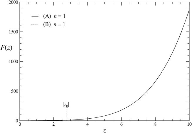
FIG. 2.: The scaling function $F(z)$.

Larger differences between the approximations given by schemes (A) and (B) for $n=1$ appear in the scaling function $f(x)$, which is shown in Fig. 3, especially in the region $x<0$, which corresponds to $t<0$ and $z$ imaginary. Note that the sizeable differences for $x>0$ are essentially caused by the normalization of $f(x)$, which is performed at the coexistence curve $x=-1$ and at the critical point $x=0$, by requiring $f(-1)=0$ and $f(0)=1$. Although the large-$x$ region corresponds to small values of $z$, the difference between the two approximate schemes does not decrease in the large-$x$ limit due to their slightly different estimates of $R_{\chi}$ (see Table XVI). Indeed, for large values of $x$

$$f(x)\sim R_{\chi}^{-1}x^{\gamma}.$$ (89)

In Fig. 3 we also plot the curve obtained in Ref. [62] by fitting the MC data.

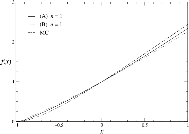
FIG. 3.: The scaling function $f(x)$. The MC curve is taken from Ref. [62].

TABLE XVI.: Universal ratios of amplitudes computed using $\alpha=-0.0146(8)$, $\eta=0.0380(4)$, $r_{6}=1.950(15)$ and $r_{8}=1.44(10)$, $r_{10}=-13(7)$. The numbers of the first four lines correspond to central values of the input parameters. The errors reported are only related to the uncertainty on the input parameters. Numbers marked with an asterisk are inputs, not predictions.

	[(A) $n=1$; $r_{6},r_{8}$]	[(B) $n=1$; $r_{6},r_{8}$]	[(A) $n=2$; $r_{6},r_{8},R_{\chi}$]	[(B) $n=2$; $r_{6},r_{8},r_{10}$]
$\rho$	2.22974	2.06825	2.23092	2.04
$\theta_{0}^{2}$	3.88383	2.93941	3.88686	2.70
$c_{1}$	$-$0.0260296	0.0758028	$-$0.0265055	0.11
$c_{2}$	0	0	0.0002163	0.01
$A^{+}/A^{-}$	1.062(4)	1.064(4)	1.062(3)	1.062(5)
$R_{\xi}^{+}$	0.355(3)	0.350(1)	0.355(2)	0.354(5)
$R_{c}$	0.127(6)	0.115(2)	0.126(2)	0.119(8)
$R_{\chi}$	1.35(7)	1.50(2)	∗1.356	1.45(8)
$R_{4}$	7.5(2)	7.92(8)	7.49(6)	7.8(3)
$F_{0}^{\infty}$	0.0302(3)	0.0300(2)	0.0302(2)	0.0302(4)
$r_{10}$	$-$10(1)	$-$11.9(1.4)	$-$10(1)	${}^{*}-$13(7)
$c_{f}$	4(2)	52(20)	4(2)

In Table XVI we report the results for some universal ratios of amplitudes. The notations are explained in App. C. The reported errors refer only to the uncertainty of the input parameters and do not include the systematic error of the procedure, which may be determined by comparing the results of the various approximations. Comparing the results for $R_{\chi}$ and $c_{f}$ with the MC estimates of Ref. [62], we observe that the parametrization (A) is in better agreement with the numerical data. This is also evident from Fig. 3.

We also consider both schemes with $n=2$. If we use $r_{10}$ to determine the next coefficient $c_{2}$, scheme (A) is not particularly useful because it is very sensitive to $r_{10}$, whose estimate has a relatively large error [26]. This fact was already observed in Ref. [26], and explained by considerations on the more complicated analytic structure. One may instead determine $c_{2}$ by using the MC result $R_{\chi}=1.356(4)$. The estimates of the universal amplitude ratios obtained in this way are presented in Table XVI. They are very close to the $n=1$ case, providing additional support to our estimates and error bars. Scheme (B) is less sensitive to $r_{10}$ and provides reasonable results if we use $r_{10}$ to fix the coefficient $c_{2}$ in $h(\theta)$ and impose the consistency condition $\theta_{0}<\theta_{l}$. The results are shown in Table XVI, where one observes that they get closer to the estimates obtained by using scheme (A).

As already mentioned, the most interesting quantity is the specific-heat amplitude ratio $A^{+}/A^{-}$, because its estimate can be compared with experimental result. Our results for $A^{+}/A^{-}$ are quite stable and insensitive to the different approximations of the equation of state we have considered, essentially because they are obtained from the function $g(\theta)$, which is not very sensitive to the local behavior of the equation of state, see Eq. (76). From Table XVI we obtain the estimate

$$A^{+}/A^{-}=1.062(4).$$ (90)

In Table XVII we compare our result (denoted by IHT-PR) with other available estimates. Note that there is a marginal disagreement with the result of Ref. [26], i.e., $A^{+}/A^{-}=1.055(3)$, which was obtained using the same method but with different input parameters: $\alpha=-0.01285(38)$ (the experimental estimate of Ref. [1]), $\eta=0.0381(3)$, $r_{6}=1.96(2)$, $r_{8}=1.40(15)$ and $r_{10}=-13(7)$. This discrepancy is mainly due to the different value of $\alpha$, since the ratio $A^{+}/A^{-}$ is particularly sensitive to it. This fact is also suggested by the phenomenological relation [63] $A^{+}/A^{-}\approx 1-4\alpha$.

We observe a discrepancy with the experimental result reported in Refs. [1, 4], $A^{+}/A^{-}=1.0442$. However, we note that in the analysis of the experimental data of Ref. [1] the estimate of $A^{+}/A^{-}$ was strongly correlated to that of $\alpha$; indeed $A^{+}/A^{-}$ was obtained by analyzing the high- and low-temperature data with $\alpha$ fixed to the value obtained from the low-temperature data alone. Therefore the slight discrepancy for $A^{+}/A^{-}$ that we observe is again a direct consequence of the differences in the estimates of $\alpha$.

For the other universal amplitude ratios we quote as our final estimates the results obtained by using scheme (A) with $n=1$:

$$R_{\xi}^{+}\equiv(A^{+})^{1/3}f^{+}=0.355(3),$$ (91)

$$R_{c}\equiv{\alpha A^{+}C^{+}\over B^{2}}=0.127(6),$$ (92)

$$R_{\chi}\equiv{C^{+}B^{\delta-1}\over(\delta C^{c})^{\delta}}=1.35(7),$$ (93)

$$R_{4}\equiv-{C_{4}^{+}B^{2}\over(C^{+})^{3}}=|z_{0}|^{2}=7.5(2),$$ (94)

$$F_{0}^{\infty}\equiv\lim_{z\rightarrow\infty}z^{-\delta}F(z)=0.0302(3),$$ (95)

$$c_{f}=4(2).$$ (96)

These results are substantially equivalent to those reported in Ref. [26].

TABLE XVII.: Estimates of $A^{+}/A^{-}$ obtained in different approaches.

IHT–PR	$d$=3 exp.	$\epsilon$-exp.	experiments
1.062(4)	1.056(4)[64]	1.029(13)[65]	1.0442 [1, 4]${}^{\ref{foot:exp}}$
1.055(3)[26]			1.067(3) [41]
			1.058(4) [42]
			1.088(7) [66]

V The two-point function of the order parameter in the high-temperature phase

The critical behavior of the two-point correlation function $G(x)$ of the order parameter is relevant to the description of scattering phenomena with light and neutron sources.

In the HT critical region, the two-point function $G(x)$ shows a universal scaling behavior. For $k,m\to 0$ ($m\equiv 1/\xi$ and $\xi$ is the second-moment correlation length) with $y\equiv k^{2}/m^{2}$ fixed, we can write [67]

$$g(y)=\chi/\widetilde{G}(k).$$ (97)

The function $g(y)$ has a regular expansion in powers of $y$:

$$g(y)=1+y+\sum_{i=2}^{\infty}c_{i}y^{i}.$$ (98)

Two other quantities characterize the low-momentum behavior of $g(y)$: they are given by the critical limit of the ratios

$$S_{M} \equiv m_{\rm gap}^{2}/m^{2},$$ (99)

$$S_{Z} \equiv \chi m^{2}/Z_{\rm gap},$$ (100)

where $m_{\rm gap}$ (the mass gap of the theory) and $Z_{\rm gap}$ determine the long-distance behavior of the two-point function:

$$G(x)\approx{Z_{\rm gap}\over 4\pi|x|}e^{-m_{\rm gap}|x|}.$$ (101)

If $y_{0}$ is the negative zero of $g(y)$ that is closest to the origin, then, in the critical limit, $S_{M}=-y_{0}$ and $S_{Z}=\left.\partial g(y)/\partial y\right|_{y=y_{0}}$.

The coefficients $c_{i}$ can be related to the critical limit of appropriate dimensionless ratios of spherical moments of $G(x)$ [45, 16] and can be computed by analyzing the corresponding HT series in the $\phi^{4}$ and in the dd-XY models, which we have calculated to 20th order. We report only our final estimates of $c_{2}$ and $c_{3}$,

$$c_{2}=-3.99(4)\times 10^{-4},$$ (102)

$$c_{3}=0.09(1)\times 10^{-4},$$ (103)

and the bound

$$|c_{4}|<10^{-6}.$$ (104)

As already observed in Ref. [45], the coefficients show the pattern

$$|c_{i}|\ll|c_{i-1}|\ll...\ll|c_{2}|\ll 1\qquad\qquad{\rm for}\qquad i\geq 3.$$ (105)

Therefore, a few terms of the expansion of $g(y)$ in powers of $y$ provide a good approximation in a relatively large region around $y=0$, larger than $|y|\lesssim 1$. This is in agreement with the theoretical expectation that the singularity of $g(y)$ closest to the origin is the three-particle cut (see, e.g., Refs. [68, 69, 45]). If this is the case, the convergence radius $r_{g}$ of the Taylor expansion of $g(y)$ is $r_{g}=9S_{M}$. Since, as we shall see, $S_{M}\approx 1$, at least asymptotically we should have

$$c_{i+1}\approx-{1\over 9}c_{i}.$$ (106)

This behavior can be checked explicitly in the large-$N$ limit of the $N$-vector model [45].

Assuming the pattern (105), we may estimate $S_{M}$ and $S_{Z}$ from $c_{2}$, $c_{3}$, and $c_{4}$. We obtain

$$S_{M} = 1+c_{2}-c_{3}+c_{4}+2c_{2}^{2}+...$$ (107)

$$S_{Z} = 1-2c_{2}+3c_{3}-4c_{4}-2c_{2}^{2}+...$$ (108)

where the ellipses indicate contributions that are negligible with respect to $c_{4}$. In Ref. [45] the relation (107) has been confirmed by a direct analysis of the HT series of $S_{M}$. From Eqs. (107) and (108) we obtain

$$S_{M}=0.999592(6),\qquad\qquad S_{Z}=1.000825(15).$$ (109)

These results improve those obtained in Ref. [45] by using HT methods in the standard XY model and field-theoretic methods, such as the $\epsilon$ expansion and the fixed-dimension $g$ expansion.

For large values of $y$, the function $g(y)$ follows the Fisher-Langer law [70]

$$g(y)^{-1}={A_{1}\over y^{1-\eta/2}}\left(1+{A_{2}\over y^{(1-\alpha)/(2\nu)}}+{A_{3}\over y^{1/(2\nu)}}\right).$$ (110)

The coefficients have been computed in the $\epsilon$ expansion to three loops [69], obtaining

$$A_{1}\approx 0.92,\qquad A_{2}\approx 1.8,\qquad A_{3}\approx-2.7.$$ (111)

In order to obtain an interpolation that is valid for all values of $y$, we will use a phenomenological function proposed by Bray [69]. This approximation has the exact large-$y$ behavior and its expansion for $y\to 0$ satisfies Eq. (106). It requires the values of the exponents $\nu$, $\alpha$, and $\eta$, and the sum of the coefficients $A_{2}+A_{3}$. For the exponents we use of course the estimates obtained in this paper, while the coefficient $A_{2}+A_{3}$ is fixed using the $\epsilon$-expansion prediction $A_{2}+A_{3}=-0.9$. Bray’s phenomenological function predicts then the constants $A_{i}$ and $c_{i}$. We obtain:

$$A_{1}\approx 0.915,\qquad\qquad A_{2} \approx -24.7,\qquad\qquad A_{3}\approx 23.8,$$ (112)

$$c_{2}\approx-4.4\times 10^{-4},\qquad\qquad c_{3} \approx 1.1\times 10^{-5},\qquad\qquad c_{4}\approx-5\times 10^{-7}.$$ (113)

The results for $A_{1}$, $c_{2}$, $c_{3}$, and $c_{4}$ are in good agreement with the above-reported estimates, while $A_{2}$ and $A_{3}$ differ significantly from the $\epsilon$-expansion results (111). Notice, however, that, since $|\alpha|$ is very small, the relevant quantity in Eq. (110) is the sum $A_{2}+A_{3}$ which is, by construction, equal in Bray’s approximation and in the $\epsilon$ expansion: in other words, the function (110) does not change significantly if we use Eq. (111) or Eq. (112) for $A_{2}$ and $A_{3}$. Thus, Bray’s approximation provides a good interpolation both in the large-$y$ and small-$y$ regions.

A The Monte Carlo simulation

1 The Monte Carlo algorithm

At present the best algorithm to simulate $N$-vector systems is the cluster algorithm proposed by Wolff [71] (see Ref. [72] for a general discussion). However, the cluster update changes only the angle of the field. Therefore, following Brower and Tamayo [73], we add a local update that changes also the modulus of the field.

a The wall-cluster update

We use the embedding algorithm proposed by Wolff [71] with two major differences. First, we do not choose an arbitrary direction, but we consider changes of the signs of the first and of the second component of the fields separately. Second, we do not use the single-cluster algorithm to update the embedded model, but the wall-cluster variant proposed in Ref. [21]. In the wall-cluster update, one flips at the same time all clusters that intersect a plane of the lattice. In Ref. [21] we found for the 3D Ising model a small gain in performance compared with the single-cluster algorithm.

Note that, since the cluster update does not change the modulus of the field, identical routines can be used for the $\phi^{4}$ model and for the dd-XY model.

b The local update of the $\phi^{4}$ model

We sweep through the lattice with a local updating scheme. At each site we perform a Metropolis step, followed by an overrelaxation step and by a second Metropolis step.

In the Metropolis update, a proposal for a new field at site $x$ is generated by

$$\phi_{x}^{\prime(1)} = \phi_{x}^{(1)}+c\,(r^{(1)}-0.5),$$ (A1)

$$\phi_{x}^{\prime(2)} = \phi_{x}^{(2)}+c\,(r^{(2)}-0.5),$$ (A2)

where $r^{(1)}$ and $r^{(2)}$ are random numbers that are uniformly distributed in $[0,1)$. The proposal is accepted with probability

$$A=\mbox{min}[1,\exp(-H^{\prime}+H)].$$ (A3)

The step size $c$ is adjusted so that the acceptance rate is approximately 1/2.

The overrelaxation step is given by

$$\vec{\phi}_{x}^{\prime}=\vec{\phi}_{x}-2\,\frac{(\vec{\phi}_{x}\cdot\vec{\phi}_{n})\,\vec{\phi}_{n}}{\vec{\phi}_{n}^{2}}\,,$$ (A4)

where $\vec{\phi}_{n}=\sum_{y\in{\rm nn}(x)}\vec{\phi}_{y}$ and ${\rm nn}(x)$ is the set of the nearest neighbors of $x$. Note that this step takes very little CPU time. Therefore, it is likely that its benefit out-balances the CPU cost.

c The local update of the dd-XY model

We sweep through the lattice with a local updating scheme, performing at each site one Metropolis update followed by the overrelaxation update (A4).

In the Metropolis update, the proposal for the field $\vec{\phi}_{x}$ at the site $x$ is given by

$$\vec{\phi}_{x}^{\prime}=(0,0)\phantom{xxxxxxxx}\phantom{xx} \phantom{xx}|\vec{\phi}_{x}|=1$$ for (A5)

$$\vec{\phi}_{x}^{\prime}=(\cos(\alpha),\sin(\alpha))\phantom{xx} \phantom{xx}|\vec{\phi}_{x}|=0,$$ for (A6)

where $\alpha$ is a random number with a uniform distribution in $[0,2\pi)$. This proposal is accepted with probability

$$A(\vec{\phi}_{x}^{\prime},\vec{\phi}_{x})=\min[1,\exp(-H^{\prime}+H)]=\min[1,\exp(\beta\,\vec{\phi}_{n}\cdot(\vec{\phi}_{x}^{\prime}-\vec{\phi}_{x})+D(\vec{\phi}_{x}^{\prime 2}-\vec{\phi}_{x}^{2}))],$$ (A7)

where $\vec{\phi}_{n}=\sum_{y\in{\rm nn}(x)}\vec{\phi}_{y}$ is the sum of the nearest-neighbor spins. We will prove in Sec. A 1 e that this update leaves the Boltzmann distribution invariant.

d The update cycle

Finally, we summarize the complete update cycle:

local update sweep;

global field rotation, in which the angle is taken from a uniform distribution in $[0,2\pi)$;

6 wall-cluster updates.

The sequence of the 6 wall-cluster updates is given by the wall in 1-2, 1-3 and 2-3 plane. In each of the three cases, we update separately each component of the field.

e Proof of the stationarity of the local update of the dd-XY model

Stationarity means that the update leaves the Boltzmann distribution invariant. Since our update is local, it is sufficient to consider the conditional distribution of a single spin for given neighbors

$$P_{b}(\vec{\phi}_{x})=\frac{1}{z}\exp(\beta\,\vec{\phi}_{x}\cdot\vec{\phi}_{n}+D\vec{\phi}_{x}^{2}),$$ (A8)

where

$$z=\int d\mu(\vec{\phi}_{x})\exp(\beta\,\vec{\phi}_{x}\cdot\vec{\phi}_{n}+D\vec{\phi}_{x}^{2})$$ (A9)

and $d\mu(\vec{\phi}_{x})$ is defined in Eq. (7). We have to prove that

$$P_{b}(\vec{\phi}_{x}^{\prime})=\int d\mu(\vec{\phi}_{x})\,W(\vec{\phi}_{x}^{\prime},\vec{\phi}_{x})\,P_{b}(\vec{\phi}_{x})$$ (A10)

is satisfied, where $W$ is the update probability defined by Eqs. (A5) and (A7).

Using Eq. (7), the right-hand side of Eq. (A10) can be rewritten as

$$W(\vec{\phi}_{x}^{\prime},0)\,P_{b}(0)+\int d\Omega({\phi}_{x})\,W(\vec{\phi}_{x}^{\prime},\vec{\phi}_{x})\,P_{b}(\vec{\phi}_{x}),$$ (A11)

where $d\Omega({\phi}_{x})$ is the normalized measure on the unit circle.

Let us first consider the case $|\vec{\phi}_{x}^{\prime}|=1$. Then, we have

$$W(\vec{\phi}_{x}^{\prime},0)\,P_{b}(0)=\frac{1}{z}\,A(\vec{\phi}_{x}^{\prime},0),$$ (A12)

and

$$\int d\Omega({\phi}_{x})\,W(\vec{\phi}_{x}^{\prime},\vec{\phi}_{x})\,P_{b}(\vec{\phi}_{x}) = W(\vec{\phi}_{x}^{\prime},\vec{\phi}_{x}^{\prime})\,P_{b}(\vec{\phi}_{x}^{\prime})=(1-A(0,\vec{\phi}_{x}^{\prime}))\,P_{b}(\vec{\phi}_{x}^{\prime})$$ (A13)

$$= P_{b}(\vec{\phi}_{x}^{\prime})-\frac{1}{z}\,A(\vec{\phi}_{x}^{\prime},0),$$ (A14)

where we have used the property

$$A(0,\vec{\psi})P_{b}(\vec{\psi})=A(\vec{\psi},0)\,P_{b}(0),$$ (A15)

valid for $|\vec{\psi}|=1$. Summing the two terms we obtain Eq. (A10) as required.

For $|\vec{\phi}_{x}^{\prime}|=0$, we have

$$W(0,0)P_{b}(0)={1\over z}\left(1-\int d\Omega({\psi})\,A(\vec{\psi},0)\right),$$ (A16)

and

$$\int d\Omega({\phi}_{x})\,W(0,\vec{\phi}_{x})\,P_{b}(\vec{\phi}_{x})={1\over z}\int d\Omega({\psi})\,A(\vec{\psi},0)$$ (A17)

where we have used again Eq. (A15). Summing the two terms we obtain Eq. (A10) as required.

2 Measuring $Z_{a}/Z_{p}$

One of the phenomenological couplings that we have studied is the ratio $Z_{a}/Z_{p}$ of the partition function $Z_{a}$ of a system with anti-periodic boundary conditions (a.b.c.) in one direction and the partition $Z_{p}$ with periodic boundary conditions (p.b.c.) in all three directions. A.b.c. are obtained by multiplying the term $\vec{\phi}_{x}\vec{\phi}_{y}$ in the Hamiltonian by $-1$ for all $x=(L_{1},x_{2},x_{3})$ and $y=(1,x_{2},x_{3})$. This ratio can be obtained using the so-called boundary-flip algorithm, applied in Ref. [43] to the Ising model and generalized in Ref. [44] to general $O(N)$-invariant non-linear $\sigma$ models.

In the boundary-flip algorithm, one considers fluctuating boundary conditions, i.e., a model with partition function

$$Z_{\rm fluct}=Z_{p}+Z_{a}=\sum_{J_{b}=\pm 1}\int\mbox{D}[\phi]\,\exp\left[\beta\sum_{\left<xy\right>}J_{\left<xy\right>}\vec{\phi}_{x}\vec{\phi}_{y}+...\right],$$ (A18)

where $J_{\left<xy\right>}=J_{b}$ for $x=(L_{1},x_{2},x_{3})$ and $y=(1,x_{2},x_{3})$, and $J_{\left<xy\right>}=1$ otherwise. $J_{b}=1$ and $J_{b}=-1$ correspond to p.b.c. and a.b.c. respectively.

In this notation, the ratio of partition functions is given by

$$\frac{Z_{a}}{Z_{p}}=\frac{\langle\delta_{J_{b},-1}\rangle}{\langle\delta_{J_{b},1}\rangle},$$ (A19)

where the expectation value is taken with fluctuating boundary conditions.

In order to simulate these boundary conditions, we need an algorithm that easily allows flips of $J_{b}$. This can be done with a special version of the cluster algorithm. For both components of the field we perform the freeze (delete) operation for the links with probability

$$p_{d}=\mbox{min}[1,\exp(-2\beta J_{\left<xy\right>}\phi_{x}^{(p)}\phi_{y}^{(p)})],$$ (A20)

where $\phi_{x}^{(p)}$ is the chosen component of $\phi_{x}$. The sign of $J_{b}$ can be flipped if there exists, for the first as well as the second component of the field, no loop of frozen links with odd winding number in the first direction. In Ref. [74] it is discussed how this can be implemented. For a more formal and general discussion, see Ref. [75]. Note that for $J_{b}=-1$ the flip can always be performed. Hence, as F. Gliozzi and A. Sokal have remarked [76], the boundary flip needs not to be performed in order to determine $Z_{a}/Z_{p}$. It is sufficient to use p.b.c. and check if the flip to a.b.c. is possible. Setting $b=1$ if the boundary can be flipped and $b=0$ otherwise, we have

$$\frac{Z_{a}}{Z_{p}}=\langle b\rangle,$$ (A21)

where the expectation value is taken with p.b.c.

3 Checks of the program

a Schwinger-Dyson equations

The properties of the integration measure allow to derive an infinite set of nontrivial equations among observables of the model. Here we have used two such equations to test the correctness of the programs and the reliability of the random-number generator. For a more general discussion of such tests, see Ref. [77].

For the $\phi^{4}$ model, the partition function remains unchanged when, at site $x$, the first component of the field is shifted by $\psi$: $\phi_{x}^{(1)}\rightarrow\phi_{x}^{(1)}+\psi$. We obtain, using also the ${\rm O}(2)$ invariance

$$0 = \left.\frac{1}{Z}\frac{\partial\langle\phi_{x}^{(1)}+\psi\rangle_{\psi}}{\partial\psi}\right|_{\psi=0}$$ (A22)

$$= \beta\sum_{\mu}\langle\vec{\phi}_{x}\vec{\phi}_{x+\hat{\mu}}\rangle-\left\langle\vec{\phi}_{x}^{2}+2\lambda(\vec{\phi_{x}}^{2}-1)\vec{\phi}_{x}^{2}\right\rangle+1,$$ (A23)

where $\langle...\rangle_{\psi}$ indicates that the Boltzmann factor is taken with the shifted field at the site $x$. A second equation, which is valid for the $\phi^{4}$ model as well as for the dd-XY model, can be derived from the invariance of the measure under rotations:

$$\phi^{(1)}_{x} \rightarrow \cos(\alpha)\,\phi^{(1)}_{x}-\sin(\alpha)\,\phi^{(2)}_{x}\,,$$ (A24)

$$\phi^{(2)}_{x} \rightarrow \sin(\alpha)\,\phi^{(1)}_{x}+\cos(\alpha)\,\phi^{(2)}_{x}\,.$$ (A25)

Taking the second derivative of the partition function with respect to $\alpha$ yields

$$0=\left.\frac{1}{Z}\frac{\partial^{2}Z(\alpha)}{\partial\alpha^{2}}\right|_{\alpha=0}=\beta^{2}\left\langle\left(\sum_{y\in{\rm nn}(x)}[\phi_{x}^{1}\phi_{y}^{2}-\phi_{x}^{2}\phi_{y}^{1}]\right)^{2}\right\rangle-\beta\sum_{y\in{\rm nn}(x)}\langle\vec{\phi}_{x}\vec{\phi}_{y}\rangle,$$ (A26)

where $y\in{\rm nn}(x)$ indicates that the sum runs over the six nearest neighbors of $x$.

We checked Eq. (A22) for all our simulations of the $\phi^{4}$ model. In the simulation we averaged Eq. (A22) over all sites of the lattice to reduce the error bars. For most of the simulations the right-hand side of Eq. (A22) differed by zero by less than 2 standard deviations. Only in one case ($L=8$, $\lambda=2.2$) the difference was about 3 standard deviations. The weighted average of the right-hand side of Eq. (A22) over all our simulations is $-8(9)\times 10^{7}$. Hence, there is no indication for a program error or a problem with the random-number generator.

We implemented Eq. (A26) in all simulations of the standard XY model and, unfortunately, only in the most recent simulations of the dd-XY model. For $L=96$, $D=1.02$, and $\beta=0.56379$ we found $\beta_{m}=0.5637896(24)$ from 575,000 measurements, where

$$\beta_{m}=\frac{2\sum_{\left<xy\right>}\langle\vec{\phi}_{x}\vec{\phi}_{y}\rangle}{\sum_{x}\left\langle\left(\sum_{y\in{\rm nn}(x)}[\phi_{x}^{1}\phi_{y}^{2}-\phi_{x}^{2}\phi_{y}^{1}]\right)^{2}\right\rangle}.$$ (A27)

We have measured $\beta_{m}$ in all our simulations of the XY model. In most cases the deviation of $\beta_{m}$ from $\beta=0.454165$ was less than one standard deviation. The largest deviation was $\beta_{m}-\beta=-0.0000049(22)$ for $L=28$. The weighted average over all simulations is $\beta_{m}-\beta=-0.00000024(52)$.

Also this check does not indicate a program error or a problem with the random-number generator.

b Checks of the Taylor expansion

As a test of the MC program and of the analysis software, we simulated the $\phi^{4}$ model for $L=4$ and $\lambda=2.1$ at the following values of $\beta$: $\beta=0.485$, $0.490$, $0.495$, $0.500$, $0.505$, $0.510$, $0.515$, and $0.520$.

We computed $\bar{R}$ with $R_{1,f}=(Z_{a}/Z_{p})_{f}=0.3202$ and $R_{1,f}=(\xi_{\rm 2nd}/L)_{f}=0.5925$ and $R_{2}=U_{4}$ and $R_{2}=U_{6}$ for all these simulations, using a third-order Taylor expansion. The results for $\bar{R}$ are summarized in Table XVIII. They show that there is a large interval in which the method works: indeed, the results for $\bar{R}$ for $\beta_{s}=0.505$, $0.510$ and $0.515$ agree within two standard deviations, although the variation of $U_{4}$ and $U_{6}$ at $\beta_{s}$ is several hundred standard deviations. In addition we have gained information about the range of $\beta$ where the extrapolation works with the desired accuracy:

$$|\beta_{s}-\beta_{f}|<0.005\times(L/4)^{1/\nu}.$$ (A28)

The factor $(L/4)^{1/\nu}$ takes care of the fact that the slope of the couplings $R$ scales like $L^{1/\nu}$. We have carefully checked that this requirement is always fulfilled in our simulations. Therefore, we are confident that the extrapolation in $\beta$, using the Taylor expansion, is implemented correctly.

TABLE XVIII.: Test of the Taylor expansion. Simulations with $L=4$, $\beta_{f}\approx 0.50773$ for $(Z_{a}/Z_{p})_{f}$, and $\beta_{f}\approx 0.50994$ for $(\xi_{\rm 2nd}/L)_{f}$. In the first column we give the value $\beta_{s}$ where the simulations have been performed (i.e., the configurations have been generated with a weight proportional to the Boltzmann factor that corresponds to $\beta_{s}$). In the columns 2 up to 5 we give the results for four choices of $\bar{R}$. These choices are labelled by $R_{2}$ at $R_{1,f}$. Finally in columns 6 and 7 we give $U_{4}$ and $U_{6}$ at $\beta_{s}$ for comparison.

$\beta_{s}$	$U_{4}$ at $(Z_{a}/Z_{p})_{f}$	$U_{6}$ at $(Z_{a}/Z_{p})_{f}$	$U_{4}$ at $(\xi_{\rm 2nd}/L)_{f}$	$U_{6}$ at $(\xi_{\rm 2nd}/L)_{f}$	$U_{4}$ at $\beta_{s}$	$U_{6}$ at $\beta_{s}$
0.485	1.249912(46)	1.76951(17)	1.239726(58)	1.73513(21)	1.360445(71)	2.17525(28)
0.490	1.249589(42)	1.76749(15)	1.239863(51)	1.73434(18)	1.334375(67)	2.07444(25)
0.495	1.249431(40)	1.76671(14)	1.239866(46)	1.73396(16)	1.309184(63)	1.98000(23)
0.500	1.249343(39)	1.76634(14)	1.239805(43)	1.73364(15)	1.284661(60)	1.89063(22)
0.505	1.249365(39)	1.76642(13)	1.239824(41)	1.73370(14)	1.261574(57)	1.80882(20)
0.510	1.249458(40)	1.76678(14)	1.239885(40)	1.73394(13)	1.239660(54)	1.73318(18)
0.515	1.249373(42)	1.76641(14)	1.239802(39)	1.73359(13)	1.218859(50)	1.66302(17)
0.520	1.249313(45)	1.76616(15)	1.239804(39)	1.73358(13)	1.199535(47)	1.59940(15)

4 CPU-time, acceptance rate, cluster size, and autocorrelation times

We have used ANSI C to implement our simulation programs. We have used our own implementation of the G05CAF random-number generator from the NAG-library. The G05CAF is a linear congruential random-number generator with modulus $m=2^{59}$, multiplier $a=13^{13}$ and increment $c=0$. Most of our simulations have been performed on 450 MHz Pentium III PCs running the Linux operating system.

For $D=1.03$, the average size of the clusters per volume decreases from about $0.52$ for $L=5$ to about $0.14$ for $L=80$. For large lattices the behavior of the size of the wall clusters per volume is roughly given by $1.198\times L^{-0.488}$. For $\lambda=2.1$ we get $1.276\times L^{-0.488}$.

The acceptance rate of the local update of the dd-XY model at $D=1.03$ is about $0.273$ for $L=5$. It increases slowly and reaches about $0.309$ for $L=80$. At the same time the density of $\vec{\phi}=(0,0)$ spins increases from about $0.150$ to $0.16628$.

The acceptance rate of the local update of the $\phi^{4}$ model at $\lambda=2.1$ is about $0.395$ for $L=5$ and increases to $0.4098$ for $L=80$. We have chosen a step size $c=2.0$ throughout.

For the dd-XY model for $16\leq L\leq 80$ one cycle of the update plus the measurement takes about $L^{3}\times 3.3\times 10^{-6}$ seconds on a 450 MHz Pentium III CPU. In this range of lattice sizes the decrease of the wall-cluster size per volume and the increase of memory access times seems to cancel almost exactly (by chance).

Roughly $2/3$ of the CPU-time is spent with the cluster update (which incorporates the measurements needed for $Z_{a}/Z_{p}$). Again about $2/3$ of the remaining time is spent in the local update.

The CPU time required for the update of the $\phi^{4}$ model is slightly larger due to a different local update and due to slightly larger wall clusters than in the dd-XY model.

In total about 5 years on a single 450 MHz Pentium III CPU were used for our study. (We had 8 CPUs available for the study.)

We performed additional runs of the $\phi^{4}$ model at $\lambda=2.1$ and $\beta=0.50915$ and the dd-XY model at $D=1.03$ and $\beta=0.5628$, where we had stored all measurements of the square of the local field, the energy, the magnetization, $F$, and the boundary variable. Hence, we could compute autocorrelation functions and times from these data. We simulated lattices of size $L=8$ up to $L=64$ for this purpose. In all cases we performed 200,000 measurements. A measurement was performed after each update cycle.

Our results for the integrated autocorrelation times are summarized in Table XIX. All autocorrelation times are given in units of measurements. We see that the autocorrelation times slightly increase with increasing $L$. At a given lattice size, the autocorrelation times for the $\phi^{4}$ model are a little smaller than those for the dd-XY model. Likely, this is caused by the particular implementation of the local updates. Among the observables that we have studied, the energy has the largest autocorrelation time. It is interesting to note that the autocorrelation time of $\sum_{x}\vec{\phi_{x}}^{2}$ shows no sign of severe critical slowing down, despite the fact that $\sum_{x}\vec{\phi_{x}}^{2}$ is only changed by the local update.

TABLE XIX.: Integrated autocorrelation times for the $\phi^{4}$ model at $\lambda=2.1$ and $\beta=0.50915$, and the dd-XY model at $D=1.03$ and $\beta=0.5628$. We have always performed 200,000 cycles. The autocorrelation times are given in units of update cycles. $\tau_{E}$ is the integrated autocorrelation time of $\sum_{\left<xy\right>}\vec{\phi}_{x}\vec{\phi}_{y}$, $\tau_{\phi^{2}}$ of $\sum_{x}\vec{\phi}^{2}_{x}$, $\tau_{\chi}$ of the magnetic susceptibility, $\tau_{F}$ of the Fourier transform of the field at minimal nonvanishing momentum, and $\tau_{b}$ of the boundary variable. “trunc” gives the time at which the summation of the autocorrelation function was truncated. Note that trunc was chosen to be the same for all observables.

$L$	$\tau_{E}$	$\tau_{\phi^{2}}$	$\tau_{\chi}$	$\tau_{F}$	$\tau_{b}$	trunc
$\phi^{4}$ model
8	2.61(5)	2.36(4)	2.30(4)	0.79(1)	1.67(3)	15
12	3.12(6)	2.72(5)	2.68(5)	0.86(2)	1.90(4)	18
16	3.39(7)	2.85(6)	2.81(6)	0.89(2)	1.99(4)	20
24	4.06(9)	3.25(7)	3.31(7)	0.94(2)	2.29(5)	25
32	4.54(11)	3.51(9)	3.57(9)	0.94(2)	2.53(6)	30
48	5.65(15)	4.22(11)	4.23(11)	1.01(2)	2.93(8)	35
64	5.89(17)	4.36(12)	4.26(12)	1.01(3)	3.08(9)	40
dd-XY model
8	2.80(4)	1.78(3)	2.47(4)	0.78(1)	1.79(3)	15
12	3.21(6)	2.01(4)	2.74(5)	0.81(2)	1.91(3)	18
16	3.57(7)	2.25(5)	2.97(5)	0.88(2)	2.13(4)	20
24	4.23(10)	2.66(6)	3.44(8)	0.93(2)	2.42(5)	25
32	4.92(12)	3.14(7)	3.83(10)	0.99(2)	2.75(6)	30
48	5.81(15)	3.65(10)	4.17(11)	0.97(3)	2.95(8)	35
64	6.58(19)	4.24(12)	4.55(13)	1.01(3)	3.22(9)	40

B Analysis of the high-temperature expansions

In this appendix we report a detailed discussion of our HT analyses. This detailed description should allow the reader to understand how we determined our estimates and the reliability of the errors we report, which are to some extent subjective.

1 Definitions and HT series

Using the linked-cluster expansion technique, we computed the 20th-order HT expansion of the magnetic susceptibility

$$\chi=\sum_{x}\langle\phi_{\alpha}(0)\phi_{\alpha}(x)\rangle,$$ (B1)

of the second moment of the two-point function

$$m_{2}=\sum_{x}x^{2}\langle\phi_{\alpha}(0)\phi_{\alpha}(x)\rangle,$$ (B2)

and therefore, of the second-moment correlation length

$$\xi^{2}={m_{2}\over 6\chi}.$$ (B3)

Moreover, we calculated the HT expansion of the zero-momentum connected $2j$-point Green’s functions $\chi_{2j}$

$$\chi_{2j}=\sum_{x_{2},...,x_{2j}}\langle\phi_{\alpha_{1}}(0)\phi_{\alpha_{1}}(x_{2})...\phi_{\alpha_{j}}(x_{2j-1})\phi_{\alpha_{j}}(x_{2j})\rangle_{c}$$ (B4)

($\chi=\chi_{2}$). More precisely, we computed $\chi_{4}$ to 18th order, $\chi_{6}$ to 17th order, $\chi_{8}$ to 16th order, and $\chi_{10}$ to 15th order. The series for the $\phi^{4}$ Hamiltonian with $\lambda=2.07$ and the dd-XY model with $D=1.02$ are reported in Tables XX and XXI. The HT series of the zero-momentum four-point coupling $g_{4}$ and of the coefficients $r_{2j}$ that parametrize the equation of state can be computed using their definitions in terms of $\chi_{2j}$ and $\xi^{2}$, i.e.,

TABLE XX.: Coefficients of the HT expansion of $m_{2}$, $\chi$, $\chi_{4}$, $\chi_{6}$,, $\chi_{8}$, and $\chi_{10}$. They have been computed using the $\phi^{4}$ Hamiltonian with $\lambda=2.07$.

$i$	$\mu_{2}$	$\chi_{2}$	$\chi_{4}$
0	0	0.82195468340525626553069	$-$0.18234682673209145113698
1	1.01341425235775258955047	2.02682850471550517910095	$-$1.79856993883835218414950
2	4.99788354573054604609481	4.39836023278442865137831	$-$10.1455394390643744635266
3	17.0521428795050699809477	9.45608303384639636168661	$-$44.4379274874486579169902
4	50.2802232377961742954821	19.7509483421835061143003	$-$166.911247402827967481247
5	136.081955345771888598704	41.0953224517675210993058	$-$566.231817578861031037728
6	349.014986520228913452360	84.3784681474012731739965	$-$1783.81074566131415934408
7	861.072204516234675501406	172.831419974338990927678	$-$5314.73425458572561425498
8	2065.11115559310738635122	351.412467687273478895617	$-$15153.8054671243945401658
9	4843.65801296852863958594	713.327141375620774069366	$-$41706.6393990107185189143
10	11163.1410843891753269547	1441.29537543678062498269	$-$111480.350225534613432415
11	25357.2828059634753398090	2908.62198285250042113961	$-$290779.553330813045449802
12	56914.8160479537305800002	5851.22700855642135604880	$-$742792.316757751368697227
13	126448.957588634753901037	11759.8313973078166535503	$-$1863674.70918289087066236
14	278504.794338270260511244	23580.6969253332410696568	$-$4603313.91229513488724197
15	608775.044038619834901124	47248.9211902315365277418	$-$11214943.2818348822933596
16	1321948.27688188944339553	94508.3475046413360663308	$-$26991439.1725436301683188
17	2853823.94933643220583008	188924.811397083165660961	$-$64258568.1525362515312215
18	6128960.82003386821732524	377150.816225492759953104	$-$151492730.104215500664052
19	13101467.5362982920867821	752534.725866450821199491
20	27889129.6761627014637264	1499898.13514730628043402
$i$	$\chi_{6}$	$\chi_{8}$	$\chi_{10}$
0	0.41197816889670188853628	$-$2.04244608438484921752518	17.4966181373390399118217
1	8.09031485009238719234751	$-$65.5324533503954629382215	827.907846284122870554505
2	80.5579033480687931078788	$-$993.099544110386544944672	17583.1558423294442666385
3	569.040955700888943670354	$-$10125.9430216092445934264	242162.737636025061958065
4	3235.75380473965447264355	$-$79870.4410385967305759821	2508010.66864972545742050
5	15823.8724636340283846359	$-$524859.679867495864300189	21148750.0733186453907577
6	69189.8243270623365490494	$-$3005237.58408599956662949	152451568.855786252573448
7	277430.904691458150896928	$-$15443601.8321215251366505	970471959.824139222337835
8	1038008.04844006612521747	$-$72717890.9115560213984880	5582186363.05878798571648
9	3669720.02487068188513696	$-$318510657.462768013289640	29507970388.4631661994252
10	12374182.7602063550019508	$-$1312668767.17043587616989	145203489229.461390006077
11	40084338.4384102309965122	$-$5135470803.97668705323439	671866031736.491009927361
12	125446404.887628912440242	$-$19206423870.3058981804587	2946715041148.83369711661
13	381003987.146313729964559	$-$69057827061.9724837730205	12330196249913.8306690405
14	1127156412.88952101681812	$-$239824993302.080594778804	49488831955055.0830738902
15	3257906807.50792443987963	$-$807540440278.527392223891	191378645936343.575972510
16	9223412391.97191941389912	$-$2645013087720.90303565763
17	25631282620.7774958190658

TABLE XXI.: Coefficients of the HT expansion of $m_{2}$, $\chi$, $\chi_{4}$, $\chi_{6}$,, $\chi_{8}$, and $\chi_{10}$. They have been computed using the dd-XY Hamiltonian with $D=1.02$.

$i$	$\mu_{2}$	$\chi_{2}$	$\chi_{4}$
0	0	0.73497259946651881066155	$-$0.12952381667498436104661
1	0.81027708294985783008938	1.62055416589971566017876	$-$1.14235747481325709236407
2	3.57318872366283058263222	3.19240289872507821851086	$-$5.86566452750871250322137
3	11.0006482367650529136739	6.24412164584056694746990	$-$23.4964691362678107734860
4	29.3868020693268986850123	11.8078991080110710061038	$-$80.6562687454557047131467
5	72.0537292098720051000559	22.2452167397051997713027	$-$249.761461812242731292855
6	167.391323293772704647731	41.3083108337880277068933	$-$717.220908333053642342640
7	373.956365385479749391430	76.5360051001560916440577	$-$1945.68221342894368675090
8	811.915341705911027278243	140.679660885119763690958	$-$5046.15791369304901147071
9	1723.52034635335232533650	258.178251744079668880881	$-$12622.3575801936426660898
10	3594.34333565606104441219	471.478755943757026593209	$-$30642.5601039304090869577
11	7386.64345245316356464020	860.010504587591344158158	$-$72548.9796473949259402584
12	14997.4679478666032080397	1563.48753262138558216805	$-$168135.618026803729643010
13	30136.9726456923668836816	2839.86987807993137143111	$-$382565.790192788611922604
14	60029.1887398932204011553	5145.84503638874703629194	$-$856629.943580595646246982
15	118656.316956262327168223	9317.67206591240832596126	$-$1891351.24076972180490224
16	232979.699867454031093529	16841.0660076130187494565	$-$4124166.11180668899412336
17	454746.664171304150538747	30421.5573167338465805825	$-$8893532.37374656560556900
18	882960.924794534410812953	54875.4729390613106530869	$-$18987953.9690154439591383
19	1706330.67007276458833100	98938.9870168970865371838
20	3283569.77023650242548276	178182.095750601905570976
$i$	$\chi_{6}$	$\chi_{8}$	$\chi_{10}$
0	0.19923804166181643967757	$-$0.67796674603175173967960	4.06523419917732615691360
1	3.64240617023376584468207	$-$20.6297276122379010898516	182.870340299506381670926
2	33.7843552454418076210054	$-$295.585300853935935335485	3697.42581896510915833415
3	221.913477156277495814452	$-$2838.14010017098792994188	48330.0439419608161526720
4	1169.53606787476515583468	$-$20984.8625853355842977237	472993.887593911146392516
5	5284.11768819259530573126	$-$128723.340916169008103149	3752687.19462636307477999
6	21286.1074543663282451107	$-$685456.078166050751079896	25350793.0882363704732840
7	78446.3667728434480782029	$-$3265581.01409539304748618	150699914.609020169056435
8	269224.069430361947223693	$-$14216412.9210915918573320	806981988.823436545704567
9	871590.289814654747926984	$-$57438991.7197952962871671	3960575199.72383885451240
10	2687478.50894078411160055	$-$217927113.188388756606030	18052318528.0576344450433
11	7951104.44962467048194209	$-$783550202.710253766125616	77211058033.5079429953492
12	22703108.4838172682261707	$-$2689172405.44915075129067	312454827813.125173762158
13	62855482.2396162632890035	$-$8861507312.08886862026490	1204410146707.71423350686
14	169374342.873715022154662	$-$28171979758.2629139055303	4446806950469.81858484485
15	445613055.420361814905254	$-$86751935057.8910676591399	15798640107921.6847945606
16	1147647339.61141521962212	$-$259625721060.742527022681
17	2899724764.50550187290555

$$g_{4}=-{3N\over N+2}{\chi_{4}\over\chi^{2}\xi^{3}},$$ (B5)

and

$$r_{6}= 10-{5(N+2)\over 3(N+4)}{\chi_{6}\chi_{2}\over\chi_{4}^{2}},$$ (B6)

$$r_{8}= 280-{280(N+2)\over 3(N+4)}{\chi_{6}\chi_{2}\over\chi_{4}^{2}}+{35(N+2)^{2}\over 9(N+4)(N+6)}{\chi_{8}\chi_{2}^{2}\over\chi_{4}^{3}},$$ (B7)

$$r_{10}= 15400-{7700(N+2)\over(N+4)}{\chi_{6}\chi_{2}\over\chi_{4}^{2}}+{350(N+2)^{2}\over(N+4)^{2}}{\chi_{6}^{2}\chi_{2}^{2}\over\chi_{4}^{4}}$$ (B9)

$$+\;{1400(N+2)^{2}\over 3(N+4)(N+6)}{\chi_{8}\chi_{2}^{2}\over\chi_{4}^{3}}-{35(N+2)^{3}\over 3(N+4)(N+6)(N+8)}{\chi_{10}\chi_{2}^{3}\over\chi_{4}^{4}}.$$

The formulae relevant for the XY universality class are obtained setting $N=2$.

2 Critical exponents

In order to determine the critical exponents $\gamma$ and $\nu$ from the HT series of $\chi$ and $\xi^{2}/\beta$ respectively, we used quasi-diagonal first-, second-, and third-order integral approximants (IA1’s, IA2’s and IA3’s respectively). Since the most precise results are obtained by using the MC estimates of $\beta_{c}$ to bias the approximants, we shall report only the results of the biased analyses. The values of $\beta_{c}$ used in the analyses are reported in Table XXII.

TABLE XXII.: MC estimates of $\beta_{c}$.

	$\beta_{c}$
$\lambda=2.00$	0	.5099049(15)
$\lambda=2.07$	0	.5093853(24)
$\lambda=2.10$	0	.5091507(13)
$\lambda=2.20$	0	.5083366(24)
$D=0.90$	0	.5764582(24)
$D=1.02$	0	.5637972(21)
$D=1.03$	0	.5627975(14)
$D=1.20$	0	.5470377(26)

Given an $n$th-order series $f(\beta)=\sum_{i=0}^{n}c_{i}\beta^{i}$, its $k$th-order integral approximant $[m_{k}/m_{k-1}/.../m_{0}/l]$ IA$k$ is a solution of the inhomogeneous $k$th-order linear differential equation

$$P_{k}(\beta)f^{(k)}(\beta)+P_{k-1}(\beta)f^{(k-1)}(\beta)+...+P_{1}(\beta)f^{(1)}(\beta)+P_{0}(\beta)f(\beta)+R(\beta)=0,$$ (B10)

where the functions $P_{i}(\beta)$ and $R(\beta)$ are polynomials of order $m_{i}$ and $l$ respectively, which are determined by the known $n$th-order small-$\beta$ expansion of $f(\beta)$ (see, e.g., Ref. [10]).

We consider three types of biased IA$k$’s:

(i) The first kind of biased IA$k$’s, which will be denoted by bIA$k$’s, is obtained by setting

$$P_{k}(\beta)=\left(1-\beta/\beta_{c}\right)p_{k}(\beta),$$ (B11)

where $p_{k}(\beta)$ is a polynomial of order $m_{k}-1$.

(ii) Since on bipartite lattices $\beta=-\beta_{c}$ is also a singular point associated to the antiferromagnetic critical behavior [78], we consider IA$k$’s with

$$P_{k}(\beta)=\left(1-\beta^{2}/\beta_{c}^{2}\right)p_{k}(\beta),$$ (B12)

where $p_{k}(\beta)$ is a polynomial of order $m_{k}-2$. We will denote them by b_±IA$k$’s.

(iii) Following Fisher and Chen [19], we also consider IA$k$’s where the polynomial associated with the highest derivative of $f(\beta)$ is even, i.e., it is a polynomial in $\beta^{2}$. In this case $m_{k}$ is the order of the polynomial $P_{k}$ as a function of $\beta^{2}$, i.e., $P_{k}\equiv\sum_{j=0}^{m_{k}}c_{j}\beta^{2j}$. Thus, in order to bias the singularity at $\beta_{c}$, we write

$$P_{k}(\beta)=\left(1-\beta^{2}/\beta_{c}^{2}\right)p_{k}(\beta^{2}),$$ (B13)

where $p_{k}(\beta)$ is a polynomial in $\beta^{2}$ of order $m_{k}-1$. We will denote them by bFCIA$k$’s.

In our analyses we consider diagonal or quasi-diagonal approximants, since they are expected to give the most accurate results. Below, we give the rules we used to select the quasi-diagonal approximants. We introduce a parameter $q$ that determines the degree of off-diagonality allowed (see below). In order to check the stability of the results with respect to the order of the series, we also perform analyses in which we average over the results obtained with series of different length. For this purpose, we introduce a parameter $p$ and perform analyses in which we use all approximants obtained from series of $\bar{n}$ terms with $n\geq\bar{n}\geq n-p$.

We consider the following sets of IA$k$’s:

(a) $[m_{1}/m_{0}/k]$ bIA1’s with

$$n\geq m_{1}+m_{0}+k+1\geq n-p,$$ (B14)

$${\rm Max}\left[\lfloor(n-1)/3\rfloor-q,3\right]\leq m_{1},m_{0},k\leq\lceil(n-1)/3\rceil+q.$$ (B15)

(b) $[m_{1}/m_{0}/k]$ b_±IA1’s with

$$n\geq m_{1}+m_{0}+k\geq n-p,$$ (B16)

$${\rm Max}\left[\lfloor(n-1)/3\rfloor-q,3\right]\leq m_{1},m_{0},k\leq\lceil(n-1)/3\rceil+q.$$ (B17)

(c) $[m_{1}/m_{0}/k]$ bFCIA1’s with

$$n\geq m_{1}+m_{0}+k+1\geq n-p,$$ (B18)

$${\rm Max}\left[\lfloor(n-1)/3\rfloor-q,3\right]\leq m_{1},m_{0},k\leq\lceil(n-1)/3\rceil+q.$$ (B19)

(d) $[m_{2}/m_{1}/m_{0}/k]$ bIA2’s with

$$n\geq m_{2}+m_{1}+m_{0}+k+3\geq n-p,$$ (B20)

$${\rm Max}\left[\lfloor(n-3)/4\rfloor-q,2\right]\leq m_{2}-1,m_{1},m_{0},k\leq\lceil(n-3)/4\rceil+q.$$ (B21)

(e) $[m_{2}/m_{1}/m_{0}/k]$ b_±IA2’s with

$$n\geq m_{2}+m_{1}+m_{0}+k+2\geq n-p,$$ (B22)

$${\rm Max}\left[\lfloor(n-3)/4\rfloor-q,2\right]\leq m_{2}-2,m_{1},m_{0},k\leq\lceil(n-3)/4\rceil+q.$$ (B23)

(f) $[m_{2}/m_{1}/m_{0}/k]$ bFCIA2’s with

$$n\geq m_{2}+m_{1}+m_{0}+k+3\geq n-p,$$ (B24)

$${\rm Max}\left[\lfloor(n-3)/4\rfloor-q,2\right]\leq m_{2}-1,m_{1},m_{0},k\leq\lceil(n-3)/4\rceil+q.$$ (B25)

(g) $[m_{3}/m_{2}/m_{1}/m_{0}/k]$ bIA3’s with

$$n\geq m_{3}+m_{2}+m_{1}+m_{0}+k+5\geq n-p,$$ (B26)

$${\rm Max}\left[\lfloor(n-5)/5\rfloor-q,2\right]\leq m_{3}-1,m_{2},m_{1},m_{0},k\leq\lceil(n-5)/5\rceil+q.$$ (B27)

In the following we fix $q=3$ for the IA1’s and $q=2$ for the IA2’s and IA3’s.

For each set of IA$k$’s we calculate the average of the values corresponding to all nondefective IA$k$’s listed above. Approximants are considered defective when they have singularities close to the real $\beta$ axis near the critical point. More precisely, we consider defective those approximants that have singularities in the rectangle

$$x_{\rm min}\leq{\rm Re}\,\beta/\beta_{c}\leq x_{\rm max},\qquad|{\rm Im}\,\beta/\beta_{c}|\leq y_{\rm max}.$$ (B28)

The values of $x_{\rm min}$, $x_{\rm max}$ and $y_{\rm max}$ are fixed essentially by stability criteria, and may differ in the various analyses. One should always check that the results depend very little on the chosen values of $x_{\rm min}$, $x_{\rm max}$, and $y_{\rm max}$, by varying them within a reasonable and rather wide range of values. The domain (B28) cannot be too large, otherwise only few approximants are left. In this case the analysis would be less robust and therefore less reliable. We introduce a parameter $s$ such that

$$x_{\rm min}=1-s,\qquad x_{\rm max}=1+s,\qquad y_{\rm max}=s,$$ (B29)

and we present results for various values of $s$. We also discard some nondefective IA’s—we call them outliers—whose results are far from the average of the other approximants. Such approximants are eliminated algorithmically: first, we compute the average $A$ and the standard deviation $\sigma$ of the results using all nondefective IA’s. Then, we discard those IA’s whose results differ by more than $n_{\sigma}\sigma$ from $A$ with $n_{\sigma}=2$. We repeat the procedure on the remaining IA’s, by calculating the new $A$ and $\sigma$, but now eliminating the IA’s whose results differ by more than $n_{\sigma}\sigma$ with $n_{\sigma}=3$. The procedure is again repeated, increasing $n_{\sigma}$ by one at each step. This procedure converges rapidly and, as we shall see, the outliers so determined are always a very small part of the selected nondefective IA’s.

In the Tables XXIII and XXIV, we present the results for the critical exponents $\gamma$ and $\nu$ respectively, obtained from the HT analysis of the $\phi^{4}$ Hamiltonian. In the Tables XXV and XXVI we report the results for the HT analysis of the dd-XY model. There we also quote the “approximant ratio” $r_{a}\equiv(g-f)/t$, where $t$ is the total number of approximants in the given set, $g$ is the number of nondefective approximants, and $f$ is the number of outliers which are discarded using the above-presented algorithm; $g-f$ is the number of “good” approximants used in the analysis; notice that $g\gg f$, and $g-f$ is never too small. For each analysis, beside the corresponding estimate, we report two numbers. The number in parentheses, $e_{1}$, is basically the spread of the approximants for $\beta_{c}$ fixed at the MC estimate. It is the standard deviation of the results obtained from all “good” IA’s divided by the square root of $r_{a}$, i.e., $e_{1}=\sigma/\sqrt{r_{a}}$. Such a definition of $e_{1}$ is useful to compare results obtained from different subsets of approximants of the same type, obtained imposing different constraints. The number in brackets, $e_{2}$, is related to the uncertainty on the value of $\beta_{c}$ and it is estimated by varying $\beta_{c}$ in the range $[\beta_{c}-\Delta\beta_{c},\beta_{c}+\Delta\beta_{c}]$.

TABLE XXIII.: Results for $\gamma$ obtained from the analysis of the 20th-order HT series of $\chi$ for the $\phi^{4}$ Hamiltonian. The number $n$ of terms used in the analysis is indicated explicitly when it is smaller than the number of available terms ($n=20$). $p=0$ when its value is not explicitly given.

$\lambda$	approximants	$r_{a}$	$\gamma$
2.00	bIA1s=1/2	$(28-2)/48$	1	.31755(11)[19]
	bIA2s=1/2	$(82-5)/115$	1	.31749(9)[17]
2.07	bIA1s=1/4	$(35-3)/48$	1	.31786(14)[30]
	bIA1s=1/2	$(28-2)/48$	1	.31785(10)[29]
	bIA1s=1	$(19-1)/48$	1	.31784(10)[28]
	bIA1p=3,s=1/2	$(103-1)/172$	1	.31766(21)[24]
	b±IA1s=1/4	$(36-2)/48$	1	.31789(20)[28]
	b±IA1s=1/2	$(21-1)/48$	1	.31789(22)[28]
	bFCIA1s=1/4	$(36-4)/48$	1	.31775(10)[28]
	bFCIA1s=1/2	$(35-4)/48$	1	.31775(9)[28]
	bIA2s=1/8	$(99-7)/115$	1	.31780(9)[27]
	bIA2s=1/4	$(93-4)/115$	1	.31780(9)[27]
	bIA2s=1/2	$(87-4)/115$	1	.31780(8)[28]
	bIA2s=1	$(60-2)/115$	1	.31781(7)[27]
	bIA2n=19,s=1/2	$(48-6)/70$	1	.31777(10)[28]
	bIA2n=18,s=1/2	$(53-4)/62$	1	.31768(9)[28]
	bIA2p=3,s=1/2	$(277-18)/345$	1	.31772(14)[25]
	bIA2p=3,s=1	$(192-5)/345$	1	.31773(14)[25]
	b±IA2s=1/2	$(46-3)/100$	1	.31781(29)[23]
	bFCIA2s=1/2	$(91-2)/140$	1	.31780(11)[29]
	bIA3s=1/2	$(56-4)/61$	1	.31787(8)[31]
2.10	bIA1s=1/2	$(29-2)/48$	1	.31777(9)[16]
	bIA2s=1/2	$(92-2)/115$	1	.31773(6)[15]
	bIA2p=3,s=1/2	$(295-17)/345$	1	.31769(10)[14]
	b±IA2s=1/2	$(49-5)/100$	1	.31774(20)[15]
	bFCIA2s=1/2	$(92-5)/140$	1	.31772(15)[17]
2.20	bIA1s=1/2	$(31-3)/48$	1	.31809(7)[30]
	bIA2s=1/2	$(94-6)/115$	1	.31807(3)[27]

TABLE XXIV.: Results for $\nu$ obtained from the analysis of the 19th-order HT series of $\xi^{2}/\beta$ for the $\phi^{4}$ Hamiltonian. The number $n$ of terms used in the analysis is indicated explicitly when it is smaller than the number of available terms ($n=19$). $p=0$ when its value is not explicitly given.

$\lambda$	approximants	$r_{a}$	$\nu$
2.00	bIA1s=1/2	$36/37$	0	.67140(2)[9]
	bIA2s=1/2	$(63-6)/70$	0	.67141(4)[8]
2.07	bIA1s=1/2,1	$36/37$	0	.67161(2)[13]
	bIA1n=18,s=1/2	$30/36$	0	.67160(4)[13]
	bIA1n=17,s=1/2	$(30-1)/33$	0	.67163(11)[12]
	bIA1p=3,s=1/2	$(124-5)/134$	0	.67162(5)[12]
	bIA1p=3,s=1	$(120-6)/134$	0	.67162(5)[12]
	b±IA1s=1/2	$(33-1)/36$	0	.67161(2)[13]
	bFCIA1s=1/2	$(29-3)/37$	0	.67158(10)[12]
	bIA2s=1/2	$(66-5)/70$	0	.67161(4)[12]
	bIA2s=1	$(50-3)/70$	0	.67162(4)[12]
	bIA2n=18,s=1/2	$(44-3)/62$	0	.67162(5)[12]
	bIA2n=17,s=1/2	$(38-2)/49$	0	.67166(4)[11]
	bIA2p=3,s=1/2	$(180-6)/215$	0	.67164(6)[12]
	bIA2p=3,s=1	$(145-7)/215$	0	.67164(5)[12]
	b±IA2s=1/2	$(55-3)/55$	0	.67161(3)[13]
	bFCIA2s=1/2	$(60-4)/85$	0	.67161(11)[14]
	bIA3s=1/2	$(17-1)/34$	0	.67159(6)[14]
2.10	bIA1s=1/2	$36/37$	0	.67160(2)[8]
	bIA2s=1/2	$(63-5)/70$	0	.67161(4)[8]
2.20	bIA1s=1/2	$36/37$	0	.67182(3)[14]
	bIA2s=1/2	$(60-4)/70$	0	.67183(7)[14]

TABLE XXV.: Results for $\gamma$ obtained from the analysis of the 20th-order HT series of $\chi$ for the dd-XY model. $p=0$ when its value is not explicitly given.

$D$	approximants	$r_{a}$	$\gamma$
0.90	bIA1s=1/2	$(35-1)/48$	1	.31685(29)[24]
	bIA2s=1/2	$(66-3)/115$	1	.31693(28)[27]
1.02	bIA1s=1/4	$(46-2)/48$	1	.31745(20)[21]
	bIA1s=1/2	$(41-3)/48$	1	.31746(17)[22]
	bIA1s=1	$(24-1)/48$	1	.31748(15)[23]
	bIA1p=3,s=1/2	$(162-9)/172$	1	.31733(35)[20]
	b±IA1s=1/2	$(35-2)/48$	1	.31735(13)[22]
	bFCIA1s=1/2	$(31-4)/48$	1	.31745(21)[22]
	bIA2s=1/4	$(103-3)/115$	1	.31748(25)[23]
	bIA2s=1/2	$(68-1)/115$	1	.31748(16)[22]
	bIA2s=1	$(22-1)/115$	1	.31754(20)[20]
	bIA2p=3,s=1/2	$(259-7)/345$	1	.31730(26)[19]
	b±IA2s=1/2	$(74-3)/100$	1	.31754(26)[22]
	bFCIA2s=1/2	$(69-4)/140$	1	.31738(38)[18]
	bIA3s=1/2	$(41-1)/61$	1	.31776(19)[24]
1.03	bIA1s=1/2	$(40-3)/48$	1	.31747(15)[14]
	bIA2s=1/2	$(71-1)/115$	1	.31751(13)[15]
	bIA2p=3,s=1/2	$(263-11)/345$	1	.31733(22)[13]
	b±IA2s=1/2	$(73-2)/100$	1	.31756(24)[13]
	bFCIA2s=1/2	$(72-4)/140$	1	.31744(27)[11]
	bIA3s=1/2	$(41-2)/61$	1	.31776(16)[16]
1.20	bIA1s=1/2	$(43-1)/48$	1	.31867(20)[28]
	bIA2s=1/2	$(99-4)/115$	1	.31868(10)[25]

TABLE XXVI.: Results for $\nu$ obtained from the analysis of the 19th-order HT series of $\xi^{2}/\beta$ for the dd-XY model. $n=19$ and $p=0$ when not explicitly given.

$D$	approximants	$r_{a}$	$\nu$
0.90	bIA1s=1/2	$(33-2)/37$	0	.67091(6)[12]
	bIA2s=1/2	$(62-3)/70$	0	.67092(10)[12]
1.02	bIA1s=1/2	$(35-3)/37$	0	.67146(7)[10]
	bIA1s=1	$(30-1)/37$	0	.67147(5)[10]
	bIA1n=18,s=1/2	$(32-1)/36$	0	.67148(15)[10]
	bIA1n=17,s=1/2	$(31-2)/33$	0	.67132(28)[9]
	bIA1p=3,s=1/2	$(124-11)/134$	0	.67143(12)[10]
	bIA1p=3,s=1	$(103-9)/134$	0	.67145(10)[10]
	b±IA1s=1/2	$(34-1)/36$	0	.67143(5)[11]
	bFCIA1s=1/2	$(33-3)/37$	0	.67136(12)[10]
	bIA2s=1/2	$(64-1)/70$	0	.67144(5)[10]
	bIA2s=1	$(55-3)/70$	0	.67145(4)[10]
	bIA2n=18,s=1/2	$(54-2)/62$	0	.67145(11)[10]
	bIA2n=17,s=1/2	$(48-5)/49$	0	.67137(3)[9]
	bIA2p=3,s=1/2	$(198-9)/215$	0	.67141(8)[9]
	b±IA2s=1/2	$(53-9)/55$	0	.67144(2)[10]
	bFCIA2s=1/2	$(78-8)/85$	0	.67140(6)[11]
	bIA3s=1/2	$(34-4)/34$	0	.67149(5)[10]
1.03	bIA1s=1/2	$(34-2)/37$	0	.67149(7)[8]
	bIA2s=1/2	$(67-4)/70$	0	.67147(5)[7]
1.20	bIA1s=1/2	$(30-1)/37$	0	.67231(12)[13]
	bIA1s=1/2	$(64-4)/70$	0	.67236(7)[12]

The results of the analyses are quite stable: all sets of IA’s give substantially consistent results. The comparison of the results obtained using all available terms of the series with those using less terms (in the Tables the number of terms is indicated explicitly when it is smaller than the number of available terms) and those obtained for $p=3$ (i.e., using $n,n-1,n-2$, and $n-3$ terms in the series) shows that the results are also stable with respect to the order of the HT series. Therefore, we do not need to perform problematic extrapolations in the number of terms, or rely on phenomenological arguments, typically based on other models, suggesting when the number of terms is sufficient to provide a reliable estimate.

From the intermediate results reported in Tables XXIII, XXIV, XXV and XXVI (which, we stress, are determined algorithmically once chosen the set of IA$k$’s), we obtain the estimates of $\gamma$ and $\nu$.

From the analyses for the $\phi^{4}$ Hamiltonian at $\lambda=2.07$, we obtain

$$\gamma=1.31780(10)[28]+0.003(\lambda-2.07),$$ (B30)

$$\nu=0.67161(5)[12]+0.002(\lambda-2.07).$$ (B31)

As before, the number between parentheses is basically the spread of the approximants at $\lambda=2.07$ using the central value of $\beta_{c}$, while the number between brackets gives the systematic error due to the uncertainty on $\beta_{c}$. Eqs. (B30) and (B31) show also the dependence of the results on the chosen value of $\lambda$. The coefficient is estimated from the results for $\lambda=2.2$ and $\lambda=2.0$, i.e., from the ratio

$${Q(\lambda=2.2)-Q(\lambda=2.0)\over 0.2},$$ (B32)

where $Q$ represents the quantity at hand. Using $\lambda^{*}=2.07(5)$, we obtain finally

$$\gamma=1.31780(10)[28]\{15\},\qquad\qquad\nu=0.67161(5)[12]\{10\},$$ (B33)

where the error due to the uncertainty on $\lambda^{*}$ is reported between braces.

Since for $\lambda=2.10$ a more precise estimate of $\beta_{c}$ is available, it is interesting to perform the same analysis, using the HT series of the $\phi^{4}$ model at $\lambda=2.10$. We obtain

$$\gamma=1.31773(10)[15]+0.003(\lambda-2.10),$$ (B34)

$$\nu=0.67160(5)[8]+0.002(\lambda-2.10),$$ (B35)

which, using $\lambda^{*}=2.07(5)$, give

$$\gamma=1.31764(10)[15]\{15\},\qquad\qquad\nu=0.67154(5)[8]\{10\},$$ (B36)

in perfect agreement with the results obtained at $\lambda=2.07$. The slight difference of the central values is essentially due to the independent estimates of $\beta_{c}$.

From the analyses for the dd-XY model at $D=1.02$, we have

$$\gamma=1.31748(20)[22]+0.006(D-1.02),$$ (B37)

$$\nu=0.67145(10)[10]+0.005(D-1.02),$$ (B38)

where the coefficient determining the dependence of the results on $D$ is estimated by computing

$${Q(D=1.2)-Q(D=0.9)\over 0.3}.$$ (B39)

Since $D^{*}=1.02(3)$, we obtain the final estimates

$$\gamma=1.31748(20)[22]\{18\},\qquad\qquad\nu=0.67145(10)[10]\{15\}.$$ (B40)

Since for $D=1.03$ a more precise estimate of $\beta_{c}$ is available, it is worthwhile to repeat the analysis using the series at this value of $D$. We have

$$\gamma=1.31751(20)[15]+0.006(D-1.03),$$ (B41)

$$\nu=0.67148(10)[8]+0.005(D-1.03),$$ (B42)

which, for $D^{*}=1.02(2)$, give

$$\gamma=1.31745(20)[15]\{18\},\qquad\qquad\nu=0.67143(10)[8]\{15\},$$ (B43)

in good agreement with the results (B40).

Consistent, although significantly less precise, results are obtained from IHT analyses that do not make use of the MC estimate of $\beta_{c}$. For example, by analyzing the HT series for the $\phi^{4}$ Hamiltonian at $\lambda=2.07$, we find $\beta_{c}=0.509385(8)$, $\gamma=1.3178(8)\{3\}$, $\nu=0.6716(4)\{1\}$, where the error in parentheses is the spread of the approximants and the error between braces corresponds to the uncertainty on $\lambda^{*}$. Here, we determine $\beta_{c}$ and $\gamma$ from the analysis of $\chi$, using IA2’s, FCIA2’s, and IA3’s, and $\nu$ from the analysis of $\xi^{2}$ using bIA2’s biased with the estimate of $\beta_{c}$ obtained in the HT analysis of $\chi$.

From the results for $\gamma$ and $\nu$, one can obtain $\eta$ by the scaling relation $\gamma=(2-\eta)\nu$. This gives $\eta=0.0379(10)$, where the error is estimated by considering the errors on $\gamma$ and $\nu$ as independent, which is of course not true. We can obtain an estimate of $\eta$ with a smaller, yet reliable, error using the so-called critical-point renormalization method (CPRM) (see Ref. [9] and references therein). In the CPRM, given two series $D(x)$ and $E(x)$ that are singular at the same point $x_{0}$, $D(x)=\sum_{i}d_{i}x^{i}\sim(x_{0}-x)^{-\delta}$ and $E(x)=\sum_{i}e_{i}x^{i}\sim(x_{0}-x)^{-\epsilon}$, one constructs a new series $F(x)=\sum_{i}(d_{i}/e_{i})x^{i}$. The function $F(x)$ is singular at $x=1$ and for $x\to 1$ behaves as $F(x)\sim(1-x)^{-\phi}$, where $\phi=1+\delta-\epsilon$. Therefore, the difference $\delta-\epsilon$ can be obtained by analyzing the expansion of $F(x)$ by means of biased approximants with a singularity at $x_{c}=1$. In order to check for possible systematic errors, we applied the CPRM to the series of $\xi^{2}/\beta$ and $\chi$ (analyzing the corresponding 19th-order series) and to the series of $\xi^{2}$ and $\chi$ (analyzing the corresponding 20th-order series). We used IA’s biased at $x_{c}=1$. In Table XXVII we present the results of several sets of IA’s. For the $\phi^{4}$ model at $\lambda=2.07$ we obtain

$$\eta\nu=0.02550(20)+0.0013(\lambda-2.07).$$ (B44)

Thus, taking into account that $\lambda^{*}=2.07(5)$, we find

$$\eta\nu=0.02550(20)\{7\},$$ (B45)

where the first error is related to the spread of the IA’s and the second one to the uncertainty on $\lambda^{*}$, evaluated as before. Analogously, for the dd-XY model we find

$$\eta\nu=0.02550(40)+0.004(D-1.02),$$ (B46)

and therefore, using $D^{*}=1.02(3)$,

$$\eta\nu=0.02550(40)\{12\},$$ (B47)

where again the first error is related to the spread of the IA’s, while the second one is related to the uncertainty on $D^{*}$.

TABLE XXVII.: Results for $\eta$ obtained using the CPRM: $(a)$ applied to $\xi^{2}/\beta$ and $\chi$ (19 orders); $(b)$ applied to $\xi^{2}$ and $\chi$ (20 orders).

	approximants	$r_{a}$	$\eta\nu$
$\lambda=2.00$	(a) bIA1s=1/2	$33/37$	0	.02547(7)
	(a) bIA2s=1/2	$(47-1)/70$	0	.0256(2)
	(b) bIA2s=1/2	$(99-9)/115$	0	.0251(3)
$\lambda=2.07$	(a) bIA1s=1/2	$37/37$	0	.02555(7)
	(a) bIA2s=1/2	$47/70$	0	.0257(2)
	(a) bIA3s=1/2	$(20-1)/34$	0	.0255(2)
	(b) bIA2s=1/2	$(96-8)/115$	0	.0252(3)
	(b) bIA3s=1/2	$(51-2)/61$	0	.0253(5)
$\lambda=2.20$	(a) bIA1s=1/2	$33/37$	0	.02573(7)
	(a) bIA2s=1/2	$(49-2)/70$	0	.0259(3)
	(b) bIA2s=1/2	$(95-11)/115$	0	.0252(3)
$D=0.90$	(a) bIA2s=1/2	$(45-1)/70$	0	.0252(3)
	(b) bIA2s=1/2	$(84-3)/115$	0	.0248(9)
$D=1.02$	(a) bIA1s=1/2	$(22-1)/37$	0	.0256(9)
	(a) bIA2s=1/2	$(37-1)/70$	0	.0257(3)
	(a) bIA3s=1/2	$(23-2)/34$	0	.0252(5)
	(b) bIA2s=1/2	$(93-3)/115$	0	.0252(8)
	(b) bIA3s=1/2	$(59-3)/61$	0	.0253(4)
$D=1.20$	(a) bIA2s=1/2	$(33-2)/70$	0	.0263(3)
	(b) bIA2s=1/2	$(96-4)/115$	0	.0259(8)

3 Amplitude ratios

In the following we describe the analysis method we employed to evaluate zero-momentum renormalized couplings, such as $g_{4}$ and $r_{2j}$. In the case of $g_{4}$ we analyzed the series $\beta^{3/2}g_{4}=\sum_{i=0}^{17}a_{i}\beta^{i}$.

Consider an amplitude ratio $A$ which, for $t\equiv\beta_{c}/\beta-1\to 0$, behaves as

$$A(t)=A^{*}+c_{1}t^{\Delta}+c_{2}t^{\Delta_{2}}+...\,.$$ (B48)

In order to determine $A^{*}$ from the HT series of $A(t)$, we consider biased IA1’s, whose behavior at $\beta_{c}$ is given by (see, e.g., Ref. [9])

$${\rm IA1}\approx f(\beta)\left(1-\beta/\beta_{c}\right)^{\zeta}+g(\beta),$$ (B49)

where $f(\beta)$ and $g(\beta)$ are regular at $\beta_{c}$, except when $\zeta$ is a non-negative integer. In particular,

$$\zeta={P_{0}(\beta_{c})\over P_{1}^{\prime}(\beta_{c})},\qquad\qquad g(\beta_{c})=-{R(\beta_{c})\over P_{0}(\beta_{c})}.$$ (B50)

In the case we are considering, $\zeta$ is positive and therefore, $g(\beta_{c})$ provides an estimate of $A^{*}$. Moreover, for improved Hamiltonians we expect $\zeta=\Delta_{2}\approx 2\Delta$ and $\Delta\approx 0.5$. In our analyses we consider bIA1’s and b_±IA1’s (see Eqs. (B15) and (B17)) and impose various constraints on the value of $\zeta$ by selecting bIA1’s with $\zeta$ larger than a given nonnegative value.

In Table XXVIII we report the results obtained for $g_{4}$ using different sets of approximants. In this case the variation due to the uncertainty of $\beta_{c}$ is negligible. Therefore, we report only the average of the results of the “good” IA1’s and their standard deviation (divided by $\sqrt{r_{a}}$) calculated at $\beta_{c}$. In Table XXVIII we also report the value of $\zeta$ obtained from the selected IA1’s. The comparison of the results for different values of $\lambda$ and $D$ shows that the errors due to uncertainty on $\lambda^{*}$ and $D^{*}$ are small and negligible.

TABLE XXVIII.: Results for $g_{4}$, obtained from the analysis of the 17th-order series of $\beta^{-3/2}g_{4}(\beta)$.

	approximants	$r_{a}$	$g_{4}$		$\zeta$
$\lambda=2.00$	bIA1s=1/4,ζ>0	$(41-1)/43$	21	.16(7)	1.	1(5)
	b±IA1s=1/4,ζ>0	$(40-2)/44$	21	.14(6)	1.	3(8)
$\lambda=2.07$	bIA1s=1/10,1/4,ζ>0	$(41-2)/43$	21	.17(6)	1.	2(5)
	bIA1s=1/4,ζ>0.5	$(38-2)/43$	21	.16(6)	1.	2(5)
	bIA1s=1/4,1.3>ζ>0.7	$23/43$	21	.19(5)	1.	0(2)
	bIA1p=2,s=1/4,ζ>0	$(105-4)/118$	21	.14(7)	1.	7(8)
	b±IA1s=1/10,1/4,ζ>0	$(40-3)/44$	21	.14(5)	1.	4(9)
	b±IA1s=1/4,ζ>0.5	$(39-2)/44$	21	.14(5)	1.	4(9)
	b±IA1s=1/4,1.3>ζ>0.7	$(20-1)/44$	21	.16(3)	1.	1(1)
	b±IA1p=2,s=1/4,ζ>0	$(80-3)/97$	21	.13(7)	2	(2)
$\lambda=2.10$	bIA1s=1/4,ζ>0	$(41-2)/43$	21	.17(6)	1.	2(5)
	bIA1s=1/4,ζ>0.5	$(38-1)/43$	21	.17(6)	1.	2(5)
	bIA1s=1/4,1.3>ζ>0.7	$23/43$	21	.19(5)	1.	0(2)
	bIA1p=2,s=1/4,ζ>0	$(105-4)/118$	21	.14(7)	1.	7(8)
	b±IA1s=1/4,ζ>0	$(39-2)/44$	21	.16(6)	1.	4(6)
	b±IA1p=2,s=1/4,ζ>0	$(79-3)/97$	21	.14(7)	2	(2)
$\lambda=2.20$	bIA1s=1/4,ζ>0	$(40-2)/43$	21	.19(5)	1.	3(6)
	b±IA1s=1/4,ζ>0	$(39-2)/44$	21	.17(5)	1.	5(9)
$D=0.90$	bIA1s=1/4,ζ>0	$(32-1)/43$	21	.07(12)	2	(2)
	b±IA1s=1/4,ζ>0	$(35-5)/44$	21	.07(9)	1.	1(4)
$D=1.02$	bIA1s=1/10,ζ>0	$(31-2)/43$	21	.16(10)	1.	5(1.4)
	bIA1s=1/4,ζ>0	$(30-2)/43$	21	.16(10)	1.	5(1.4)
	bIA1s=1/4,ζ>0.5	$(24-1)/43$	21	.13(6)	1.	7(1.4)
	bIA1s=1/4,1.3>ζ>0.7	$9/43$	21	.16(7)	0.	9(2)
	bIA1p=2,s=1/4,ζ>0	$(69-8)/118$	21	.2(3)	1.	6(1.3)
	b±IA1s=1/4,ζ>0	$(36-3)/44$	21	.13(7)	1.	5(1.0)
	b±IA1s=1/4,ζ>0.5	$(32-4)/44$	21	.11(5)	1.	5(8)
	b±IA1s=1/4,1.3>ζ>0.7	$(16-1)/44$	21	.13(3)	1.	1(1)
	b±IA1p=2,s=1/4,ζ>0	$(66-7)/97$	21	.13(12)	2	(2)
$D=1.03$	bIA1s=1/4,ζ>0	$(32-3)/43$	21	.17(12)	1.	5(1.5)
	b±IA1s=1/4,ζ>0	$(36-3)/44$	21	.13(6)	1.	6(1.1)
$D=1.20$	bIA1s=1/4,ζ>0	$(34-4)/43$	21	.23(3)	3	(3)
	b±IA1s=1/4,ζ>0	$(33-2)/44$	21	.23(3)	2	(2)

From the results of Table XXVIII we derive the estimates

$$g_{4}=21.15(6),\qquad\qquad g_{4}=21.13(7),$$ (B51)

respectively for the $\phi^{4}$ Hamiltonian and the dd-XY model. We note that these results are slightly larger than the estimates reported in Ref. [26]. The difference is essentially due to the different analysis employed. There, the analysis was based on Padé (PA), Dlog-Padé (DPA) and IA1’s, selecting those without singularities in a neighborhood of $\beta_{c}$ and evaluating them at $\beta_{c}$. However, by analyzing the longer series that are now available for the Ising model [79], we have realized that such procedure is not very accurate and that the analyses using bIA1’s are more reliable when a sufficiently large number of terms is available. Moreover, when the series is sufficiently long, most (and eventually all) PA’s, DPA’s and IA1’s become defective. Indeed, the functions we are considering do have singularities at $\beta_{c}$, although with a positive exponent.

In the analysis of $r_{2j}$, we also consider PA’s and DPA’s. We indeed expect that, when the series is not sufficiently long to be asymptotic, the approximants obtained by biasing the singularity at $\beta_{c}$ may not provide a robust analysis. For comparison, we also use quasi-diagonal Padé approximants (PA’s) and Dlog-Padé approximants (DPA’s), evaluating them at $\beta_{c}$.

We consider:

$[l/m]$ PA’s with

$$l+m\geq n-2,$$ (B52)

$${\rm Max}\left[n/2-q,4\right]\leq l,m\leq n/2+q,$$ (B53)

where $l,m$ are the orders of the polynomials respectively in the numerator and denominator of the PA. As estimate from the PA’s we take the average of the values at $\beta_{c}$ of the nondefective approximants using all the available terms of the series and satisfying the condition (B53) with $q=3$. The error we quote is the standard deviation (divided by $\sqrt{r_{a}}$) of the results from all the nondefective approximants listed above. We consider defective those PA’s that have singularities in the rectangle defined in Eq. (B28) with: $x_{\rm min}=0.9$, $x_{\rm max}=1.01$, and $y_{\rm max}=0.1$ for $r_{6}$ and $r_{8}$; $x_{\rm min}=0$, $x_{\rm max}=1.1$, and $y_{\rm max}=0.1$ for $r_{10}$.

$[l/m]$ DPA’s with

$$l+m\geq n-3,$$ (B54)

$${\rm Max}\left[(n-1)/2-q,4\right]\leq l,m\leq(n-1)/2+q,$$ (B55)

where $l,m$ are the orders of the polynomials respectively in the numerator and denominator of the PA of the series of its logarithmic derivative. We again fix $q=3$. The estimate with the corresponding error is obtained as in the case of PA’s. We consider defective those DPA’s that have singularities in the rectangle (B28) with $x_{\rm min}=0$, $x_{\rm max}=1.01$, and $y_{\rm max}=0.1$.

For $r_{6}$ and $r_{8}$ the above PA’s and DPA’s give results substantially consistent with those of bIA1’s, see Tables XXIX and XXX. Therefore the systematic error due to the use of PA’s and DPA’s should be smaller than the final quoted errors. From Tables XXIX and XXX we derive the estimates reported in Table XIV. For $r_{10}$ we obtain only very rough estimates using essentially PA’s: $r_{10}=-13(7)$ from the $\phi^{4}$ Hamiltonian and $r_{10}=-11(14)$ from the dd-$XY$ model.

TABLE XXIX.: Results for $r_{6}$ from the analysis of the corresponding 17th-order HT series.

	approximants	$r_{a}$	$r_{6}$
$\lambda=2.00$	PA	$19/21$	1	.945(20)
	DPA	$12/18$	1	.959(27)
$\lambda=2.07$	PA	$19/21$	1	.947(22)
	DPA	$12/18$	1	.962(26)
	bIA1s=1/10,ζ>0	$(21-1)/43$	1	.98(10)
	bIA1s=1/10,ζ>0.5	$(17-1)/43$	1	.955(9)
	bIA1p=2,s=1/10,ζ>0	$(58-3)/118$	1	.99(9)
	bIA1p=2,s=1/10,ζ>0.5	$(42-2)/118$	1	.956(10)
$\lambda=2.10$	PA	$19/21$	1	.948(23)
	DPA	$12/18$	1	.963(26)
	bIA1s=1/10,ζ>0	$(21-1)/43$	1	.98(7)
	bIA1s=1/10,ζ>0.5	$(18-1)/43$	1	.959(19)
$\lambda=2.20$	PA	$19/21$	1	.951(30)
	DPA	$13/18$	1	.967(26)
$D=0.90$	PA	$21/21$	1	.934(15)
	DPA	$16/18$	1	.936(11)
$D=1.02$	PA	$20/21$	1	.945(13)
	DPA	$12/18$	1	.952(13)
	bIA1s=1/10,ζ>0	$(28-1)/43$	1	.948(11)
	bIA1s=1/10,ζ>0.5	$(27-1)/43$	1	.947(8)
	bIA1p=2,s=1/10,ζ>0	$(69-1)/118$	1	.947(17)
	bIA1p=2,s=1/10,ζ>0.5	$(65-1)/118$	1	.948(16)
$D=1.03$	PA	$20/21$	1	.946(8)
	DPA	$12/18$	1	.954(16)
$D=1.20$	PA	$21/21$	1	.963(6)
	DPA	$16/18$	1	.963(12)

TABLE XXX.: Results for $r_{8}$ from the analysis of the corresponding 16-th order HT series.

	approximants	$r_{a}$	$r_{8}$
$\lambda=2.00$	PA	$17/18$	1	.32(14)
	DPA	$14/21$	1	.34(22)
$\lambda=2.07$	PA	$17/18$	1	.36(14)
	DPA	$13/21$	1	.37(15)
	bIA1s=1/10,ζ>0	$(10-1)/33$	1	.39(13)
	bIA1p=2,s=1/10,ζ>0	$(33-2)/91$	1	.30(15)
$\lambda=2.10$	PA	$18/18$	1	.35(12)
	DPA	$13/21$	1	.38(12)
$\lambda=2.20$	PA	$18/18$	1	.41(12)
	DPA	$13/21$	1	.42(17)
$D=0.90$	PA	$16/18$	1	.34(18)
	DPA	$18/21$	1	.28(10)
$D=1.02$	PA	$17/18$	1	.50(14)
	DPA	$15/21$	1	.47(6)
	bIA1s=1/10,ζ>0	$(15-1)/33$	1	.45(12)
	bIA1p=2,s=1/10,ζ>0	$(45-5)/91$	1	.50(33)
$D=1.03$	PA	$17/18$	1	.52(13)
	DPA	$15/21$	1	.54(8)
$D=1.20$	PA	$16/18$	1	.64(9)
	DPA	$15/21$	1	.65(13)

C Universal amplitude ratios

We give here the definitions of the amplitude ratios that are used in the text. They are expressed in terms of the amplitudes derived from the singular behavior of the specific heat

$$C_{H}=A^{\pm}|t|^{-\alpha},$$ (C1)

the magnetic susceptibility in the high-temperature phase

$$\chi={1\over 2}C^{+}t^{-\gamma},$$ (C2)

the zero-momentum four-point connected correlation function in the high temperature phase

$$\chi_{4}={8\over 3}C_{4}^{+}t^{-\gamma-2\beta\delta},$$ (C3)

the second-moment correlation length in the high-temperature phase

$$\xi=f^{+}t^{-\nu},$$ (C4)

the spontaneous magnetization on the coexistence curve

$$M=B|t|^{\beta},$$ (C5)

and of the susceptibility along the critical isotherm

$$\chi_{L}=C^{c}|H|^{-{\gamma/\beta\delta}}.$$ (C6)

We consider the following universal amplitude ratios:

$$R_{c}\equiv{\alpha A^{+}C^{+}\over B^{2}},$$ (C7)

$$R_{4}\equiv-{C_{4}^{+}B^{2}\over(C^{+})^{3}}=|z_{0}|^{2},$$ (C8)

$$R_{\chi}\equiv{C^{+}B^{\delta-1}\over(\delta C^{c})^{\delta}},$$ (C9)

$$R_{\xi}^{+}\equiv(A^{+})^{1/3}f^{+}=\left({R_{4}R_{c}\over g_{4}}\right)^{1/3}.$$ (C10)

REFERENCES

- [1] J. A. Lipa, D. R. Swanson, J. A. Nissen, T. C. P. Chui, and U. E. Israelsson, Phys. Rev. Lett. 76, 944 (1996).
- [2] R. Guida and J. Zinn-Justin, J. Phys. A 31, 8103 (1998).
- [3] M. Hasenbusch and T. Török, J. Phys. A 32, 6361 (1999).
- [4] J. A. Lipa, D. R. Swanson, J. A. Nissen, Z. K. Geng, P. R. Williamson, D. A. Stricker, T. C. P. Chui, U. E. Israelsson, and M. Larson, Phys. Rev. Lett. 84, 4894 (2000).
- [5] J. A. Lipa, private communication.
- [6] M. Campostrini, A. Pelissetto, P. Rossi, and E. Vicari, Phys. Rev. B 61 5905 (2000).
- [7] J. A. Nissen, D. R. Swanson, Z. K. Geng, V. Dohm, U. E. Israelsson, M. J. DiPirro, and J. A. Lipa, Low Temp. Phys. 24, 86 (1998).
- [8] K. E. Newman and E. K. Riedel, Phys. Rev. B 30, 6615 (1984).
- [9] D. L. Hunter and G. A. Baker, Jr., Phys. Rev. B 7, 3346 (1973); B 7, 3377 (1973); B 19, 3808 (1979); M. E. Fisher and H. Au-Yang, J. Phys. A 12, 1677 (1979); Erratum A 13, 1517 (1980); A. J. Guttmann and G. S. Joyce, J. Phys. A 5, L81 (1972); J. J. Rehr, A. J. Guttmann, and G. S Joyce, J. Phys. A 13, 1587 (1980).
- [10] A. J. Guttmann, in Phase Transitions and Critical Phenomena, Vol. 13, edited by C. Domb and J. Lebowitz (Academic, New York, 1989).
- [11] R. Z. Roskies, Phys. Rev. B 24, 5305 (1981).
- [12] J. Adler, M. Moshe, and V. Privman, Phys. Rev. B 26, 1411 (1982); Phys. Rev. B 26, 3958 (1982).
- [13] P. Butera and M. Comi, Phys. Rev. B 56, 8212 (1997).
- [14] A. Pelissetto and E. Vicari, Nucl. Phys. B 519, 626 (1998); Nucl. Phys. B (Proc. Suppl.) 73, 775 (1999).
- [15] P. Butera and M. Comi, Phys. Rev. B 58, 11552 (1998).
- [16] M. Campostrini, A. Pelissetto, P. Rossi, and E. Vicari, Phys. Rev. E 60, 3526 (1999).
- [17] J.-H. Chen, M. E. Fisher, and B. G. Nickel, Phys. Rev. Lett. 48, 630 (1982).
- [18] M. J. George and J. J. Rehr, Phys. Rev. Lett. 53, 2063 (1984).
- [19] M. E. Fisher and J.-H. Chen, J. Physique 46, 1645 (1985).
- [20] B. G. Nickel and J. J. Rehr, J. Stat. Phys. 61, 1 (1990).
- [21] M. Hasenbusch, K. Pinn, and S. Vinti, Phys. Rev. B 59, 11471 (1999).
- [22] H. G. Ballesteros, L. A. Fernández, V. Martín-Mayor, and A. Muñoz Sudupe, Phys. Lett. B 441, 330 (1998).
- [23] H. G. Ballesteros, L. A. Fernández, V. Martín-Mayor, A. Muñoz Sudupe, G. Parisi, and J. J. Ruiz-Lorenzo, J. Phys. A 32, 1 (1999).
- [24] M. Hasenbusch, J. Phys. A 32, 4851 (1999).
- [25] M. Hasenbusch, in preparation.
- [26] M. Campostrini, A. Pelissetto, P. Rossi, and E. Vicari, Phys. Rev. B 62, 5843 (2000).
- [27] P. H. Damgaard and M. Hasenbusch, Phys. Lett. B 331, 440 (1994).
- [28] F. Jasch and H. Kleinert, “Fast convergent resummation algorithm and critical exponents of theory in three dimensions,” e-print cond-mat/9906246v2.
- [29] G. A. Baker, Jr., B. G. Nickel, M. S. Green, and D. I. Meiron, Phys. Rev. Lett. 36, 1351 (1977); G. A. Baker, Jr., B. G. Nickel, and D. I. Meiron, Phys. Rev. B 17, 1365 (1978).
- [30] D. B. Murray and B. G. Nickel, “Revised estimates for critical exponents for the continuum -vector model in 3 dimensions,” unpublished Guelph University report (1991).
- [31] K. G. Chetyrkin, S. G. Gorishny, S. A. Larin, and F. V. Tkachov, Phys. Lett. B 132, 351 (1983).
- [32] H. Kleinert, J. Neu, V. Schulte-Frohlinde, K. G. Chetyrkin, and S. A. Larin, Phys. Lett. B 272, 39 (1991); Erratum B 319, 545 (1993).
- [33] P. Butera and M. Comi, Phys. Rev. B 60, 6749 (1999).
- [34] M. Krech and D. P. Landau, Phys. Rev. B 60, 3375 (1999).
- [35] H. G. Ballesteros, L. A. Fernández, V. Martín-Mayor, and A. Muñoz Sudupe, Phys. Lett. B 387, 125 (1996).
- [36] N. Schultka and E. Manousakis, Phys. Rev. B 52, 7528 (1995).
- [37] M. Hasenbusch and A. P. Gottlob, Physica A 201, 593 (1993).
- [38] W. Janke, Phys. Lett. A 148, 306 (1990).
- [39] L. S. Goldner, N. Mulders, and G. Ahlers, J. Low Temp. Phys. 93, 131 (1993).
- [40] D. R. Swanson, T. C. P. Chui, and J. A. Lipa, Phys. Rev. B 46, 9043 (1992); D. Marek, J. A. Lipa, and D. Philips, Phys. Rev. B 38, 4465 (1988).
- [41] A. Singsaas and G. Ahlers, Phys. Rev. B 30, 5103 (1984).
- [42] J. A. Lipa and T. C. P. Chui, Phys. Rev. Lett. 51, 2291 (1983).
- [43] M. Hasenbusch, Physica A 197, 423 (1993).
- [44] A. P. Gottlob and M. Hasenbusch, J. Stat. Phys. 77, 919 (1994).
- [45] M. Campostrini, A. Pelissetto, P. Rossi, and E. Vicari, Europhys. Lett. 38, 577 (1997); Phys. Rev. E 57, 184 (1998).
- [46] V. Privman, P. C. Hohenberg, and A. Aharony, in Phase Transitions and Critical Phenomena, Vol. 14, edited by C. Domb and J. L. Lebowitz (Academic, New York, 1991).
- [47] R. Guida and J. Zinn-Justin, Nucl. Phys. B 489, 626 (1997).
- [48] J. Zinn-Justin, Quantum Field Theory and Critical Phenomena, third edition (Clarendon Press, Oxford, 1996).
- [49] E. Brézin and D. J. Wallace, Phys. Rev. B 7, 1967 (1973).
- [50] E. Brézin and J. Zinn-Justin, Phys. Rev. B 14, 3110 (1976).
- [51] I. D. Lawrie, J. Phys. A 14, 2489 (1981).
- [52] D. J. Wallace and R. P. K. Zia, Phys. Rev. B 12, 5340 (1975).
- [53] L. Schäfer and H. Horner, Z. Phys. B 29, 251 (1978).
- [54] A. Pelissetto and E. Vicari, Nucl. Phys. B 540, 639 (1999).
- [55] A. Pelissetto and E. Vicari, Nucl. Phys. B 575, 579 (2000).
- [56] T. Reisz, Phys. Lett. B 360, 77 (1995).
- [57] A. I. Sokolov, E. V. Orlov, V. A. Ul’kov, and S. S. Kastanov, Phys. Rev. E 60, 1344 (1999).
- [58] A. Pelissetto and E. Vicari, Nucl. Phys. B 522, 605 (1998).
- [59] P. Schofield, Phys. Rev. Lett. 22, 606 (1969).
- [60] P. Schofield, J. D. Lister, and J. T. Ho, Phys. Rev. Lett. 23, 1098 (1969).
- [61] B. D. Josephson, J. Phys. C: Solid State Phys. 2, 1113 (1969).
- [62] J. Engels, S. Holtmann, T. Mendes, and T. Schulze, “Equation of state and Goldstone-mode effects of the three-dimensional model,” e-print hep-lat/0006023, Phys. Lett. B, in press.
- [63] C. Hohenberg, A. Aharony, B. I. Halperin, and E. D. Siggia, Phys. Rev. B 13, 2986 (1976).
- [64] S. A. Larin, M. Mönnigman, M. Strösser, and V. Dohm, Phys. Rev. B 58, 3394 (1998).
- [65] C. Bervillier, Phys. Rev. B 34, 8141 (1986).
- [66] T. Takada and T. Watanabe, J. Low Temp. Phys. 49, 435 (1982).
- [67] M. E. Fisher and R. J. Burford, Phys. Rev. 156, 583 (1967); H. B. Tarko and M. E. Fisher, Phys. Rev. Lett. 31, 926 (1973); H. B. Tarko and M. E. Fisher, Phys. Rev. B 11, 1217 (1975); M. E. Fisher and A. Aharony, Phys. Rev. B 7, 2818 (1974).
- [68] R. A. Ferrel and D. J. Scalapino, Phys. Rev. Lett. 34, 200 (1975).
- [69] A. J. Bray, Phys. Rev. B 14, 1248 (1976).
- [70] M. E. Fisher and J. S. Langer, Phys. Rev. Lett. 20, 665 (1968).
- [71] U. Wolff, Phys. Rev. Lett. 62, 361 (1989).
- [72] S. Caracciolo, R. G. Edwards, A. Pelissetto, and A. D. Sokal, Nucl. Phys. B (Proc. Suppl.) 26, 595 (1992); Nucl. Phys. B 403, 475 (1993).
- [73] R. C. Brower and P. Tamayo, Phys. Rev. Lett. 62, 1087 (1989).
- [74] M. Hasenbusch, Habilitationsschrift, December 1999, Humboldt-Universität zu Berlin.
- [75] M. Caselle, F. Gliozzi and S. Necco, “Thermal operators and cluster topology in -state Potts Models,” e-print cond-mat/0006204.
- [76] F. Gliozzi and A. Sokal, private communication.
- [77] H. G. Ballesteros and V. Martín-Mayor, Phys. Rev. E 58, 6787 (1998).
- [78] M. E. Fisher, Philos. Mag. 7, 1731 (1962).
- [79] M. Campostrini, “Linked-Cluster Expansion of the Ising Model”, e-print cond-mat/0005130.