Oscillator Strength of Metallic Carbon Nanotubes

A carbon nanotube (CN) is composed of a coaxially rolled graphite sheet.${}^{\hbox{\immediate{\bf{?}})}}$ The materials are characterized by two integers, $(N_{+},N_{-})$, corresponding to a wrapping vector along the waist, $\vec{w}=N_{+}\vec{a}_{+}+N_{-}\vec{a}_{-}$, where $\vec{a}_{+}$ and $\vec{a}_{-}$ are primitive lattice vectors of the graphite and $|\vec{a}_{\pm}|=a$. It has been shown that the CN’s have peculiar band structures.${}^{\hbox{\immediate{\bf{?}},\penalty 1000\hskip 0.91003pt plus 0.70004pt minus 0.70004pt{\bf{?}},\penalty 1000\hskip 0.91003pt plus 0.70004pt minus 0.70004pt{\bf{?}})}}$ When $N_{+}-N_{-}=0$ mod 3, the metallic one-dimensional (1D) dispersions appear near the center of the bands. The low energy properties less than $v_{0}/R$ ($v_{0}$ : Fermi velocity, $R$ : radius of the tube ) is described by taking account of only the metallic 1D dispersions.${}^{\hbox{\immediate{\bf{?}},\penalty 1000\hskip 0.91003pt plus 0.70004pt minus 0.70004pt{\bf{?}},\penalty 1000\hskip 0.91003pt plus 0.70004pt minus 0.70004pt{\bf{?}},\penalty 1000\hskip 0.91003pt plus 0.70004pt minus 0.70004pt{\bf{?}},\penalty 1000\hskip 0.91003pt plus 0.70004pt minus 0.70004pt{\bf{?}})}}$ Correlation effects obtained by such a treatment have been observed in the transport experiment.${}^{\hbox{\immediate{\bf{?}})}}$

Carrier doping to CN’s has been done by doping the electron-donor (e.g., potassium, rubidium) or electron-acceptor (e.g., iodine, bromine). ${}^{\hbox{\immediate{\bf{?}},\penalty 1000\hskip 0.91003pt plus 0.70004pt minus 0.70004pt{\bf{?}},\penalty 1000\hskip 0.91003pt plus 0.70004pt minus 0.70004pt{\bf{?}},\penalty 1000\hskip 0.91003pt plus 0.70004pt minus 0.70004pt{\bf{?}})}}$ It has been experimentally observed that the doping changes the properties of CN’s. In bundles of single wall CN’s, bromine and potassium doping decrease the resistivity at 300K up to a factor of 30, and enlarge the region where the temperature coefficient of resistance is positive.${}^{\hbox{\immediate{?})}}$ The similar behavior is observed in a potassium-doped single rope.${}^{\hbox{\immediate{?})}}$ Change of the Ramann spectra has been observed in the bundles of CN’s with doping of K, Rb and Br₂.${}^{\hbox{\immediate{?})}}$ Enhancement of spin susceptibility due to potassium-doping has been also reported.${}^{\hbox{\immediate{?})}}$ As an another method for doping, a downward shift of the Fermi level due to the gold substrate has been reported by scanning tunneling spectroscopy.${}^{\hbox{\immediate{\bf{?}})}}$

The oscillator strength $\int_{0}^{\infty}{\rm d}\omega{\rm Re}\sigma(\omega)$, where $\sigma(\omega)$ is the optical conductivity, is closely related to the amount of carrier. Irrespective of the presence of the mutual interaction, as far as the kinetic energy is expressed by the quadratic dispersion, the oscillator strength is given as follows,

$$\int_{0}^{\infty}{\rm d}\omega{\rm Re}\sigma(\omega)=\frac{\pi}{2}\frac{ne^{2}}{m},$$ (1)

where $n$ and $m$ are the electron density and the mass, respectively. On the other hand, the oscillator strength is different from eq.(1) in the case of tight binding models.${}^{\hbox{\immediate{\bf{?}})}}$ As the simplest system, we consider a linear chain model with the nearest neighbor hopping, $t_{i,i+1}$, whose kinetic energy is given by $T=-\sum_{i,s}\{t_{i,i+1}c^{\dagger}_{i,s}c_{i+1,s}+h.c.\}$. The oscillator strength is calculated as,${}^{\hbox{\immediate{?})}}$

$$\int_{0}^{\infty}{\rm d}\omega{\rm Re}\sigma(\omega)=-\frac{\pi}{2}\frac{e^{2}d}{N_{L}}\left\langle T\right\rangle,$$ (2)

where $N_{L}$ is the number of the lattice sites, $d$ is a lattice spacing and $\left\langle\cdots\right\rangle$ is the thermal average. The quantity, $\left\langle T\right\rangle$, is not proportional to the electron density. For example, in case of $t_{i,i+1}=t$ without the mutual interaction, eq.(2) reduces to $2e^{2}td\sin(\pi dn/2)$ at the absolute zero temperature. The difference between eqs.(1) and (2) with respect to carrier dependence results from distinction of their band structures.

It is obvious that the quantities for the high energy scale such as the oscillator strength cannot be described by the theory in which only the metallic dispersions are taken into account. Ando has been calculated the optical conductivity of CN’s by using the effective mass theory, which is valid for the energy scale less than $v_{0}/a$.${}^{\hbox{\immediate{\bf{?}})}}$ He predicted that the absorption edge is shifted to the higher energy side due to Coulomb interaction, which has been observed in the recent experiment.${}^{\hbox{\immediate{\bf{?}})}}$ Thus the effective mass theory succeeds in describing the low energy physics very well. However, it is questionable whether the theory is effective for discussing the oscillator strength and it’s dependence on the amount of the carrier.

In the present paper, using the tight binding method, we derive the formulae of the oscillator strength of $(N,N)$ armchair CN’s and metallic $(N,0)$ zigzag CN’s. The formulae are compared with the result of the linear chain model, eq.(2). In addition, the doping dependence of the oscillator strength is discussed in detail${}^{\hbox{\immediate{\bf{?}})}}$ in the absence of Coulomb interaction. We take a unit of $\hbar=c=1$.

We consider the armchair and zigzag CN’s shown in Fig.1 (a) and (b), respectively.

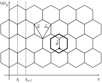
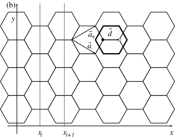
Fig.  1: Carbon atoms in armchair nanotubes (a) and zigzag nanotubes (b) where the $x$ axis points along the tube. Here $\vec{a}_{\pm}$ are two primitive lattice vectors of a graphite, and $|\vec{a}_{\pm}|=a$. The hexagon shown by the thick line is the unit cell and the black (white) circle denotes the sublattice $p=+(-)$.

Here the directions of the tube and of the waist are denoted as $x$ and $y$, respectively. An electric field is applied to the $x$-direction. The kinetic energy of the armchair CN, ${\cal H}_{\rm k}^{AN}$, in the presence of the time dependent vector potential along the $x$-direction $A(x,u)$, is given as,

$${\cal H}_{\rm k}^{AN}=\sum_{{\vec{r}}_{i},s}\left\{-ta^{\dagger}_{-,s}({\vec{r}}_{i})a_{+,s}({\vec{r}}_{i})+h.c.\right\}$$ (3)

$$+ \sum_{{\vec{r}}_{i},s}\left\{-t{\rm e}^{{\rm i}eA(x_{i},u)a/2}a^{\dagger}_{+,s}({\vec{r}}_{i})a_{-,s}({\vec{r}}_{i}-{\vec{a}}_{+})+h.c.\right\}$$

$$+ \sum_{{\vec{r}}_{i},s}\left\{-t{\rm e}^{{\rm i}eA(x_{i},u)a/2}a^{\dagger}_{-,s}({\vec{r}}_{i})a_{+,s}({\vec{r}}_{i}+{\vec{a}}_{-})+h.c.\right\},$$

where $t$ denotes the hopping integral between the nearest-neighbor atoms, and $a^{\dagger}_{p,s}({\vec{r}}_{i})$ is the creation operator of the electron with spin $s$ at the location, ${\vec{r}}_{i}-p{\vec{d}}/2$ ($p=\pm$). The electric field is given by $-\partial_{u}A(x,u)$.

The current operator $I^{AN}(x_{i})$ is obtained by differentiating eq.(3) in terms of $A(x_{i},u)$. Up to the first order of $A(x_{i},u)$,

$$I^{AN}(x_{i}) = {\rm i}et\sum_{y_{i},s}{\hbox{$\left\{\vbox to0.0pt{}\right.\n@space$}}a^{\dagger}_{+,s}(\vec{r}_{i})a_{-,s}(\vec{r}_{i}-\vec{a}_{+})$$ (4)

$$+ a^{\dagger}_{-,s}(\vec{r}_{i})a_{+,s}(\vec{r}_{i}+\vec{a}_{-})-h.c.{\hbox{$\left\}\vbox to0.0pt{}\right.\n@space$}}$$

$$- \frac{e^{2}tA(x_{i},u)a}{2}\sum_{y_{i},s}{\hbox{$\left\{\vbox to0.0pt{}\right.\n@space$}}a^{\dagger}_{+,s}(\vec{r}_{i})a_{-,s}(\vec{r}_{i}-\vec{a}_{+})$$

$$+ a^{\dagger}_{-,s}(\vec{r}_{i})a_{+,s}(\vec{r}_{i}+\vec{a}_{-})+h.c.{\hbox{$\left\}\vbox to0.0pt{}\right.\n@space$}}.$$

On the other hand, the kinetic energy of the zigzag CN,

$${\cal H}_{\rm k}^{ZN}=\sum_{{\vec{r}}_{i},s}\left\{-t{\rm e}^{{\rm i}eA(x_{i},u)a/\sqrt{3}}a^{\dagger}_{-,s}({\vec{r}}_{i})a_{+,s}({\vec{r}}_{i})+h.c.\right\}$$ (5)

$$+ \sum_{{\vec{r}}_{i},s}\left\{-t{\rm e}^{{\rm i}eA(x_{i},u)a/\sqrt{12}}a^{\dagger}_{+,s}({\vec{r}}_{i})a_{-,s}({\vec{r}}_{i}-{\vec{a}}_{+})+h.c.\right\}$$

$$+ \sum_{{\vec{r}}_{i},s}\left\{-t{\rm e}^{{\rm i}eA(x_{i},u)a/\sqrt{12}}a^{\dagger}_{+,s}({\vec{r}}_{i})a_{-,s}({\vec{r}}_{i}-{\vec{a}}_{-})+h.c.\right\},$$

leads to the current operator,

$$I^{ZN}(x_{i})=\frac{{\rm i}et}{3}\sum_{y_{i},s}{\hbox{$\left\{\vbox to0.0pt{}\right.\n@space$}}2a^{\dagger}_{-,s}(\vec{r}_{i})a_{+,s}(\vec{r}_{i})$$ (6)

$$+ a^{\dagger}_{+,s}(\vec{r}_{i})a_{-,s}(\vec{r}_{i}-\vec{a}_{+})+a^{\dagger}_{+,s}(\vec{r}_{i})a_{-,s}(\vec{r}_{i}-\vec{a}_{-})-h.c.{\hbox{$\left\}\vbox to0.0pt{}\right.\n@space$}}$$

$$- \frac{e^{2}tA(x_{i},u)a}{6\sqrt{3}}\sum_{y_{i},s}{\hbox{$\left\{\vbox to0.0pt{}\right.\n@space$}}4a^{\dagger}_{-,s}(\vec{r}_{i})a_{+,s}(\vec{r}_{i})+a^{\dagger}_{+,s}(\vec{r}_{i})a_{-,s}(\vec{r}_{i}-\vec{a}_{+})$$

$$+ a^{\dagger}_{+,s}(\vec{r}_{i})a_{-,s}(\vec{r}_{i}-\vec{a}_{-})+h.c.{\hbox{$\left\}\vbox to0.0pt{}\right.\n@space$}}.$$

The current density operator per unit length along the waist, ${j}_{2D}(x_{i})$, and that per unit area, ${j}_{3D}(x_{i})$, are given by ${j}^{C}_{2D}(x_{i})={I}^{C}(x_{i})/(2\pi R)$ and ${j}^{C}_{3D}(x_{i})={I}^{C}(x_{i})/(\pi R^{2})$, where $R=\sqrt{3}Na/(2\pi)$ and $R=Na/(2\pi)$ for $C$ = $AN$ (armchair CN’s) and $C=ZN$ (zigzag CN’s), respectively.

In order to compare the oscillator strength between the linear chain model and the CN, we calculate the oscillator strength corresponding to the 1D currents, eqs.(4) and (6). The diamagnetic component of the current, which is proportional to $A(x,u)$, leads to the oscillator strength $Z^{C}_{1D}$ :

$$Z^{C}_{1D} = -\frac{\pi}{2}\left\langle X^{C}\right\rangle,$$ (7)

where $\left\langle\cdots\right\rangle$ expresses the thermal average in the absence of the vector potential, and $X^{C}$ ($C=AN$, $ZN$) are defined as,

$$X^{AN} = -\frac{e^{2}t}{L}\left(\frac{a^{2}}{4}\right)\sum_{\vec{r}_{i}s}{\hbox{$\left\{\vbox to0.0pt{}\right.\n@space$}}a^{\dagger}_{+,s}(\vec{r}_{i})a_{-,s}(\vec{r}_{i}-\vec{a}_{+})$$ (8)

$$\hskip 20.00003pt+a^{\dagger}_{-,s}(\vec{r}_{i})a_{+,s}(\vec{r}_{i}+\vec{a}_{-})+h.c.{\hbox{$\left\}\vbox to0.0pt{}\right.\n@space$}},$$

and

$$X^{ZN}=-\frac{e^{2}t}{L}\left(\frac{a^{2}}{12}\right)\sum_{\vec{r}_{i}s}{\hbox{$\left\{\vbox to0.0pt{}\right.\n@space$}}4a^{\dagger}_{-,s}(\vec{r}_{i})a_{+,s}(\vec{r}_{i})$$

$$+ a^{\dagger}_{+,s}(\vec{r}_{i})a_{-,s}(\vec{r}_{i}-\vec{a}_{+})+a^{\dagger}_{+,s}(\vec{r}_{i})a_{+,s}(\vec{r}_{i}-\vec{a}_{-})+h.c.{\hbox{$\left\}\vbox to0.0pt{}\right.\n@space$}},$$

with $L$ being the length of the tube. The oscillator strength corresponding to the 2D and 3D current densities are given by $Z_{2D}^{C}=Z_{1D}^{C}/(2\pi R)$ and $Z_{3D}^{C}=Z_{1D}^{C}(\omega)/(\pi R^{2})$. The quantities $X^{AN}$ and $X^{ZN}$ are, respectively, not proportional to the kinetic energies eq.(3) and eq.(5) in the case of $A(x,u)=0$. It is due to the fact that the CN is not the linear chain system.

Now we calculate $Z^{C}_{1D}$ as a function of hole doping, $\delta\equiv 1-N_{e}/N_{c}$, where $N_{e}$ ($N_{c}$) is the number of electrons (carbon atoms), in the absence of Coulomb interaction. In this case, the intensity of the optical conductivity exists within the band width, i.e., $0\leq\omega\leq 6t$. The quantities, $\left\langle X^{C}\right\rangle$ and $\delta$, are determined by the following equations as a function of the chemical potential, $\mu$. For armchair CN’s,

$$\left\langle X^{AN}\right\rangle=\frac{te^{2}a^{2}}{4\pi}\int_{-2\pi/a}^{2\pi/a}{\rm d}K_{x}$$

$$\times \sum_{K_{y}}\sum_{\alpha=\pm}\alpha Z^{AN}(\vec{K})f(\alpha\xi^{AN}(\vec{K})-\mu),$$

$$\delta=\frac{a}{4N\pi}\int_{-2\pi/a}^{2\pi/a}{\rm d}K_{x}$$

$$\times \sum_{K_{y}}\sum_{\alpha=\pm}{\hbox{$\left\{\vbox to0.0pt{}\right.\n@space$}}f(\alpha\xi^{AN}(\vec{K}))-f(\alpha\xi^{AN}(\vec{K})-\mu){\hbox{$\left\}\vbox to0.0pt{}\right.\n@space$}},$$ (11)

with

$$Z^{AN}(\vec{K}) = 2t\cos(K_{x}a/2)$$ (12)

$$\times\left\{2\cos({K_{x}a}/{2})+\cos({K_{y}\sqrt{3}a}/{2})\right\}/\xi^{AN}(\vec{K}),$$

$$\xi^{AN}(\vec{K}) = t{\hbox{$\left\{\vbox to0.0pt{}\right.\n@space$}}1+4\cos^{2}({K_{x}a}/{2})$$ (13)

$$+4\cos({K_{x}a}/{2})\cos({K_{y}\sqrt{3}a}/{2}){\hbox{$\left\}\vbox to0.0pt{}\right.\n@space$}}^{1/2},$$

where ${\vec{K}}=(K_{x},K_{y})$, $K_{y}=2\pi n/(\sqrt{3}Na)$ with $n$ being $-[N/2],\cdots,[N/2]$ for odd $N$ or $-N/2,\cdots,N/2-1$ for even $N$ and $f(\epsilon)$ is the Fermi function. On the other hand, for zigzag nanotubes,

$$\left\langle X^{ZN}\right\rangle=\frac{te^{2}a^{2}}{12\pi}\int_{0}^{4\pi/(\sqrt{3}a)}{\rm d}K_{x}$$ (14)

$$\times \sum_{K_{y}}\sum_{\alpha=\pm}\alpha Z^{ZN}(\vec{K})f(\alpha\xi^{ZN}(\vec{K})-\mu),$$

$$\delta = \frac{\sqrt{3}a}{4N\pi}\int_{0}^{4\pi/\sqrt{3}a}{\rm d}K_{x}$$ (15)

$$\times \sum_{K_{y}}\sum_{\alpha=\pm}{\hbox{$\left\{\vbox to0.0pt{}\right.\n@space$}}f(\alpha\xi^{ZN}(\vec{K}))-f(\alpha\xi^{ZN}(\vec{K})-\mu){\hbox{$\left\}\vbox to0.0pt{}\right.\n@space$}},$$

with

$$Z^{ZN}(\vec{K}) = 2t{\hbox{$\left\{\vbox to0.0pt{}\right.\n@space$}}2+5\cos(K_{x}\sqrt{3}a/2)\cos K_{y}a/2$$ (16)

$$+ 2\cos^{2}K_{y}a/2{\hbox{$\left\}\vbox to0.0pt{}\right.\n@space$}}/\xi^{ZN}(\vec{K}),$$

$$\xi^{ZN}(\vec{K}) = t{\hbox{$\left\{\vbox to0.0pt{}\right.\n@space$}}1+4\cos^{2}({K_{y}a}/{2})$$ (17)

$$+4\cos({K_{y}a}/{2})\cos({K_{x}\sqrt{3}a}/{2}){\hbox{$\left\}\vbox to0.0pt{}\right.\n@space$}}^{1/2},$$

where $K_{y}=2\pi n/(Na)$ with $n$ being $-[N/2],\cdots,[N/2]$ for odd $N$ or $-N/2,\cdots,N/2-1$ for even $N$. Note that $\pm\xi^{AN}(\vec{K})$ ($\pm\xi^{ZN}(\vec{K})$) are the energy dispersions of the armchair (zigzag) CN, and those with $K_{y}=0$ ($K_{y}=\pm 2\pi/3a$) can be zero. Hereafter, such dispersions are called as center metallic bands.

$Z_{1D}^{C}/(te^{2}a)$ is shown in Fig.2 as a function of $\delta$ at the absolute zero temperature.

Fig.  2: $Z_{1D}^{C}$ in unit of $e^{2}ta$ of $(N,N)$ armchair and $(N,0)$ zigzag CN’s as a function of $\delta$ for the several choices of $N$.

Fig.  3: $Z_{2D}^{C}$ in unit of $e^{2}t$ of $(N,N)$ armchair and $(N,0)$ zigzag CN’s as a function of $\delta$ for the several choices of $N$.

$Z^{C}_{1D}$ has a maximum at half-filling ($\delta=0$) : It decreases with increasing $|\delta|$ and vanishes when the bands are empty or full ($\delta=1$ or $-1$). The fine structures are due to the Van Hove singularities of the density of states. We find that, within numerical accuracy, $Z^{C}_{2D}$ in the absence of doping ($\delta=0$) is independent of $N$ and has the same value for the armchair and zigzag CN’s, i.e., $Z^{AN}_{2D}=Z^{ZN}_{2D}\simeq 0.952e^{2}t$ as is shown in Fig.3. It seems to be related to the fact that the number of the states less than Fermi energy at $\delta=0$ for the system with the fixed tube length is proportional to $R$ and independent of chirality. The doping dependence, however, differs for each nanotube due to it’s own peculiar band structure.

Next, let us consider the doping dependence, $\Delta Z^{C}_{1D}\equiv Z^{C}_{1D}|_{\delta=0}-Z^{C}_{1D}$, in detail. In the case where the chemical potential stays at only the center metallic bands, the quantities, $\delta$ and $\Delta Z^{C}_{1D}$, can be calculated as follows : For armchair CN’s,

$$\delta = \frac{K_{+}-K_{-}}{2N\pi},$$ (18)

$$\Delta Z^{AN}_{1D} = te^{2}a\left\{\sqrt{3}-\sin K_{+}a/2-\sin K_{-}a/2\right\},$$ (19)

where $\cos K_{\pm}a/2=(\pm\mu/t-1)/2$. And for zigzag nanotubes,

$$\delta = \frac{\sqrt{3}a}{2N\pi}(K_{+}-K_{-}),$$ (20)

$$\Delta Z^{ZN}_{1D} = \frac{5}{3\sqrt{3}}te^{2}a\left\{2-\sin\frac{K_{+}\sqrt{3}a}{4}-\sin\frac{K_{-}\sqrt{3}a}{4}\right\},$$

where $\cos K_{\pm}\sqrt{3}a/4=\pm\mu/(2t)$. In the case of $|\mu/t|\ll 1$, eqs.(18)-(LABEL:eqn:DZZN) lead to

$$\Delta Z^{AN}_{1D} \simeq te^{2}a\frac{N^{2}\pi^{2}}{2\sqrt{3}}\delta^{2},$$ (22)

$$\Delta Z^{ZN}_{1D} \simeq te^{2}a\frac{5N^{2}\pi^{2}}{48\sqrt{3}}\delta^{2}.$$ (23)

Thus, $\Delta Z^{C}_{1D}$ is proportional to $\delta^{2}$ and the square of the radius of the tube. Then $\Delta Z^{C}_{3D}\equiv\Delta Z^{C}_{1D}/(\pi R^{2})$ is independent of the radius as $\Delta Z^{AN}_{3D}=(te^{2}/a)(2\pi^{3}/3\sqrt{3})\delta^{2}$ and $\Delta Z^{ZN}_{3D}=(te^{2}/a)(5\pi^{3}/12\sqrt{3})\delta^{2}$. The values of both equations are close to each other. The quantity obtained experimentally is nothing but $Z_{3D}$ because the reflectance observed experimentally is related to the optical conductivity corresponding to the 3D current density. Therefore, from the above equations, the amount of doping may be well determined even when CN’s with different chirality and radius coexist if the CN’s with the another chirality have values close to $\Delta Z^{AN}_{3D}$ and/or $\Delta Z^{ZN}_{3D}$.

In summary, we have derived the formulae of the oscillator strength of the armchair and metallic zigzag CN’s, and compared with the result of the linear chain model. Dependence of the oscillator strength on the amount of the doping has been calculated in the absence of Coulomb interaction. We have found that $Z^{C}_{2D}$ for half-filling is the same irrespective of the type of CN’s and the radius of the tube. The doping dependence, however, are different reflecting their peculiar band structures. It is found that $\Delta Z_{3D}^{C}$ is independent of the radius of the tube and the values for both CN’s are close to each other. The relation may be useful for determining the amount of doping. Here we compare the present results and those by the effective mass theory, which has been used for calculating the optical conductivity corresponding to the 2D current density for half-filling in ref.?. By integrating eq.(2.28) in ref.? in the absence of Coulomb interaction, one obtains $Z_{2D}^{EM}=(2e^{2}\gamma)/(2\pi R)\sum_{\kappa_{n}}$ for the oscillator strength for half-filling where $\kappa_{n}=n/R$ ($n=0,\pm 1,\cdots)$ for metallic CN’s and $\gamma=\sqrt{3}ta/2$. In principle, there are no upper and lower bounds for the transverse momentum $\kappa_{n}$ in the effective mass scheme. However, the number of the allowed transverse momenta is considered to be proportional to the radius of the tube if the cut-off of the order of $a^{-1}$ is introduced. Then, $Z_{2D}^{EM}$ is independent of the radius, which is qualitatively the same as that for the present study. However, there remains numerical ambiguity.

In the present analysis, we have calculated the doping dependence in the absence of Coulomb interaction. Though eq.(1) is independent of the mutual interaction, the oscillator strength of the tight binding model depends on the interaction.${}^{\hbox{\immediate{\bf{?}},\penalty 1000\hskip 0.91003pt plus 0.70004pt minus 0.70004pt{\bf{?}},\penalty 1000\hskip 0.91003pt plus 0.70004pt minus 0.70004pt{\bf{?}})}}$ Since the long range Coulomb interaction has been considered to play a crucial roles in CN’s,${}^{\hbox{\immediate{?},\penalty 1000\hskip 0.91003pt plus 0.70004pt minus 0.70004pt{?},\penalty 1000\hskip 0.91003pt plus 0.70004pt minus 0.70004pt{?},\penalty 1000\hskip 0.91003pt plus 0.70004pt minus 0.70004pt{?},\penalty 1000\hskip 0.91003pt plus 0.70004pt minus 0.70004pt{?},\penalty 1000\hskip 0.91003pt plus 0.70004pt minus 0.70004pt{?})}}$ it’s effect should be investigated.

The author would like to thank Y. Iwasa for useful comments and S. Iwabuchi for stimulating discussion and critical reading of the manuscript. This work was supported by a Grant-in-Aid for Scientific Research from the Ministry of Education, Science, Sports and Culture (No.11740196).

References

• [1] S. Iijima: Nature (London) 354 (1991) 56.
• [2] N. Hamada, S. Sawada and A. Oshiyama: Phys.Β Rev.Β Lett. 68 (1992) 1579.
• [3] R. Saito, M. Fujita, G. Dresselhaus and M. S. Dresselhaus: Phys.Β Rev.Β B 46 (1992) 1804.
• [4] R. Saito, M. Fujita, G. Dresselhaus and M. S. Dresselhaus: Appl.Β Phys.Β Lett. 60 (1992) 2204.
• [5] R. Egger and A. O. Gogolin: Phys.Β Rev.Β Lett. 79 (1997) 5082
• [6] C. L. Kane, L. Balents, and M. P. A. Fisher: Phys.Β Rev.Β Lett. 79 (1997) 5086.
• [7] R. Egger and A. O. Gogolin: Eur.Β Phys.Β J.Β B 3 (1998) 281.
• [8] H. Yoshioka and A. A. Odintsov: Phys.Β Rev.Β Lett. 82 (1999) 374.
• [9] A. A. Odintsov and H. Yoshioka: Phys.Β Rev.Β B 59 (1999) 10457.
• [10] M. Bockrath, D. H. Cobden, J. Lu, A. G. Rinzler, R. E. Smalley, L. Balents, and P. L. McEuen: Nature (London) 397 (1999) 598.
• [11] R. S. Lee, H. J. Kim, J. E. Fischer, A. Thess and R. E. Smalley: Nature (London) 388 (1997) 255.
• [12] A. M. Rao, P. C. Eklund, S. Bandow, A. Thess and R. E. Smalley: Nature (London) 388 (1997) 257.
• [13] R. S. Lee, H. J. Kim, J. E. Fischer, J. Lefebvre, M. Radosavljevi${\rm\acute{c}}$, J. Hone and A. T. Johnson: Phys.Β Rev.Β B 61 (2000) 4526.
• [14] A. S. Claye, N. M. Nemes, A. J${\rm\acute{a}}$nossy, and J. E. Fischer: Phys.Β Rev.Β B 62 (2000) R4845.
• [15] J. W. G. Wild$\ddot{\rm o}$er, L. C. Venema, A. G. Rinzler, R. E. Smalley, and C. Dekker: Nature (London) 391 (1998) 59
• [16] See, for example, R. A. Bari, D. Adler and R. V. Lange: Phys.Β Rev.Β B 2 (1970) 2898, I. Sadakata and E. Hanamura: J.Β Phys.Β Soc.Β Jpn. 34 (1973) 882, P. F. Maldague: Phys.Β Rev.Β B 16 (1977) 2437.
• [17] T. Ando: J.Β Phys.Β Soc.Β Jpn. 66 (1997) 1066.
• [18] M. Ichida, S. Mizuno, Y. Tani, Y. Saito and A. Nakamura: J.Β Phys.Β Soc.Β Jpn. 68 (1999) 3131.
• [19] In ref.?, it has been pointed out that the simple formula, eq.(1), does not hold for CN’s.
• [20] D. Baeriswyl, J. Carmelo and A. Luther: Phys.Β Rev.Β B 33 (1986) 7247.
• [21] C. S. Jacobsen: J.Β Phys.Β C 19 (1986) 5643.
• [22] F. Mila: Phys.Β Rev.Β B 52 (1995) 4788.