Optimization with Extremal Dynamics

Abstract

We explore a new general-purpose heuristic for finding high-quality solutions to hard optimization problems. The method, called extremal optimization, is inspired by self-organized criticality, a concept introduced to describe emergent complexity in physical systems. Extremal optimization successively replaces extremely undesirable variables of a single sub-optimal solution with new, random ones. Large fluctuations ensue, that efficiently explore many local optima. With only one adjustable parameter, the heuristic’s performance has proven competitive with more elaborate methods, especially near phase transitions which are believed to coincide with the hardest instances. We use extremal optimization to elucidate the phase transition in the 3-coloring problem, and we provide independent confirmation of previously reported extrapolations for the ground-state energy of $\pm J$ spin glasses in $d=3$ and $4$. PACS number(s): 02.60.Pn, 05.65.+b, 75.10.Nr, 64.60.Cn.

Many natural systems have, without any centralized organizing facility, developed into complex structures that optimize their use of resources in sophisticated ways Bakbook . Biological evolution has formed efficient and strongly interdependent networks in which resources rarely go to waste. Even the morphology of inanimate landscapes exhibits patterns that seem to serve a purpose, such as the efficient drainage of water Somfai ; rivers .

Natural systems that exhibit self-organizing qualities often possess a common feature: a large number of strongly coupled entities with similar properties. Hence, at some coarse level they permit a statistical description. An external resource (sunlight in the case of evolution) drives the system which then takes its direction purely by chance. Like descending water breaking through the weakest of all barriers in its wake, biological species are coupled in a global comparative process that persistently washes away the least fit. In this process, unlikely but highly adapted structures surface inadvertently. Optimal adaptation thus emerges naturally, from the dynamics, simply through a selection against the extremely “bad”. In fact, this process prevents the inflexibility inevitable in a controlled breeding of the “good”.

Various models relying on extremal processes have been proposed to explain the phenomenon of self-organization PMB . In particular, the Bak-Sneppen model of biological evolution is based on this principle BS ; BoPa1 . Assuming an unspecified interdependency between species, it produces salient nontrivial features of pale-ontological data such as broadly distributed lifetimes of species, large extinction events, and punctuated equilibrium.

In the Bak-Sneppen model, species are located on the sites of a lattice, and have an associated “fitness” value between 0 and 1. At each time step, the one species with the smallest value (poorest degree of adaptation) is selected for a random update, having its fitness replaced by a new value drawn randomly from a flat distribution on the interval $[0,1]$. But the change in fitness of one species impacts the fitness of interrelated species. Therefore, all of the species at neighboring lattice sites have their fitness replaced with new random numbers as well. After a sufficient number of steps, the system reaches a highly correlated state known as self-organized criticality (SOC) BTW . In that state, almost all species have reached a fitness above a certain threshold. These species, however, possess punctuated equilibrium: only one’s weakened neighbor can undermine one’s own fitness. This coevolutionary activity gives rise to chain reactions called “avalanches”, large fluctuations that rearrange major parts of the system, potentially making any configuration accessible.

Although coevolution does not have optimization as its exclusive goal, it serves as a powerful paradigm. We have used it as motivation for a new approach to optimization BoPe1 . The heuristic we have introduced, called extremal optimization (EO), follows the spirit of the Bak-Sneppen model, merely updating those variables having the “worst” values in a solution and replacing them by random values without ever explicitly improving them.

Previously, several heuristics inspired by natural processes have been proposed, notably simulated annealing Science and genetic algorithms Holland . These have aroused considerable interest among physicists, in the development of physically motivated heuristics Houdayer ; Dittes ; Moebius , and in their applications to physical problems Pal ; Hartmann_d3 ; Hartmann_d4 . EO adds a distinctly new approach to the approximation of hard optimization problems by utilizing large fluctuations inherent to systems driven far from equilibrium. In this Letter we demonstrate EO’s generality, the simplicity of its implementation, and its results, for a physical problem as well as for a classic combinatorial optimization problem. A tutorial introduction is given in Ref. CISE .

The physical problem we consider is a spin glass MPV . It consists of a $d$-dimensional hyper-cubic lattice of length $L$, with a spin variable $x_{i}\in\{-1,1\}$ at each site $i$, $1\leq i\leq n$ $(=L^{d})$. A spin is connected to each of its nearest neighbors $j$ via a bond variable $J_{ij}\in\{-1,1\}$, assigned at random. The configuration space $\Omega$ consist of all configurations $S=(x_{1},\ldots,x_{n})\in\Omega$ where $|\Omega|=2^{n}$.

We wish to minimize the cost function, or Hamiltonian

$$C(S)=H({\bf x})=-{1\over 2}{\sum\sum}_{\langle i,j\rangle}J_{ij}x_{i}x_{j}.$$ (1)

Due to frustration MPV , ground state configurations $S_{\rm min}$ are hard to find, and it has been shown that for $d>2$ the problem is among the hardest optimization problems Barahona .

To find low-energy configurations, EO assigns a fitness to each spin variable $x_{i}$

$$\lambda_{i}=x_{i}\,\left({1\over 2}\sum_{j}J_{ij}x_{j}\right),$$ (2)

so that

$$C(S)=-\sum_{i=1}^{n}\lambda_{i}.$$ (3)

Unlike in genetic algorithms, the fitness does not characterize an entire configuration, but simply a single variable of the configuration. In similarity to the Bak-Sneppen model, EO then proceeds to search $\Omega$ by sequentially changing variables with “bad” fitness at each update step. The simplest “neighborhood” $N(S)$ for an update consists of all configurations $S^{\prime}\in N(S)$ that could be reached from $S$ through the flip of a single spin. After each update, the fitnesses of the changed variable and of all its neighbors are reevaluated according to Eq. (2).

The basic EO algorithm proceeds as follows:

1. Initialize configuration $S$ at will; set $S_{\rm best}\!:=\!S$. 2. For the “current” configuration $S$, (a) evaluate $\lambda_{i}$ for each variable $x_{i}$, (b) find $j$ satisfying $\lambda_{j}\leq\lambda_{i}$ for all $i$, i.e., $x_{j}$ has the “worst fitness”, (c) choose $S^{\prime}\!\in\!N(S)$ so that $x_{j}$ must change, (d) accept $S:=S^{\prime}$ unconditionally, (e) if $C(S)<C(S_{\rm best})$ then set $S_{\rm best}:=S$. 3. Repeat at step (2) as long as desired. 4. Return $S_{\rm best}$ and $C(S_{\rm best})$.

Initial tests have shown that this basic algorithm is quite competitive for optimization problems where EO can choose randomly among many $S^{\prime}\in N(S)$ satisfying step (2c), such as graph partitioning BoPe1 . But, in cases such as the single spin-flip neighborhood above, focusing on only the worst fitness [step (2b)] leads to a deterministic process, leaving no choice in step (2c). To avoid such “dead ends” and to improve results BoPe1 , we introduce a single parameter into the algorithm. We rank all the variables $x_{i}$ according to fitness $\lambda_{i}$, i.e., find a permutation $\Pi$ of the variable labels $i$ with

$$\lambda_{\Pi(1)}\leq\lambda_{\Pi(2)}\leq\ldots\leq\lambda_{\Pi(n)}.$$ (4)

The worst variable $x_{j}$ [step (2b)] is of rank 1, $j=\Pi(1)$, and the best variable is of rank $n$. Now, consider a probability distribution over the ranks $k$,

$$P_{k}\propto k^{-\tau},\qquad 1\leq k\leq n,$$ (5)

for a given value of the parameter $\tau$. At each update, select a rank $k$ according to $P_{k}$. Then, modify step (2c) so that the variable $x_{i}$ with $i=\Pi(k)$ changes its state.

For $\tau=0$, this “$\tau$-EO” algorithm is simply a random walk through $\Omega$. Conversely, for $\tau\to\infty$, the process approaches a deterministic local search, only updating the lowest-ranked variable, and is bound to reach a dead end (see Fig. 1). However, for finite values of $\tau$ the choice of a scale-free distribution for $P_{k}$ in Eq. (5) ensures that no rank gets excluded from further evolution, while maintaining a clear bias against variables with bad fitness.

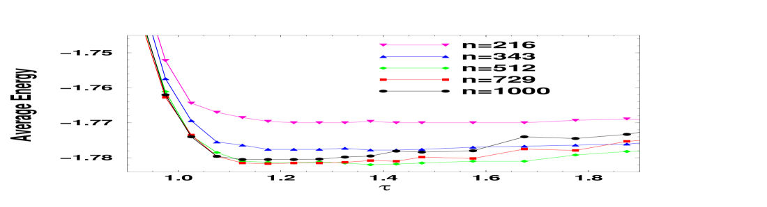
Figure 1: Plot of the average energies obtained by EO for the $\pm J$ spin glass in $d=3$ as a function of $\tau$. For each size $n$, 10 instances were chosen. For each instance, 10 EO runs were performed starting from different initial conditions at each $\tau$. The results were averaged over runs and over instances. The best results are obtained at $\tau$ moving slowly toward $\tau\to 1^{+}$ for $n\to\infty$.

For the spin glass, we obtained our best solutions for $\tau\to 1^{+}$, as shown in Fig. 1. Generally, over many optimization problems, the preferred value seems to scale slowly as $\tau-1\sim 1/\ln n$ for increasing $n$. Experiments with random graphs support this expectation BoPe2 , although the dependence on $n$ can be practically negligible. For instance, at fixed $\tau=1.4$, $\tau$-EO already reproduced many testbed results for the partitioning of graphs of sizes $n=1000$ to $n\gtrsim 10^{5}$ BoPe1 .

We have run the $\tau$-EO algorithm with $\tau=1.15$ on a large number of realizations of the $J_{ij}$, for $n=L^{d}$ with $L=5,6,7,8,9,10,12$ in $d=3$, and with $L=3,4,5,6,7$ in $d=4$. To reduce variances, we fixed $|\sum J_{ij}|\leq 1$. For each instance, we have run EO with 5 restarts from random initial conditions, retaining only the lowest energy state obtained, and then averaging over instances. Inspection of the convergence results for the genetic algorithms in Refs. Pal ; Houdayer suggest a runtime scaling at least as $n^{3}$–$n^{4}$ for consistent performance. Indeed, using $\sim n^{4}/100$ updates enables EO to reproduce its lowest energy states on about 80% to 95% of the restarts, for each $n$. Our results are listed in Table 1. A fit of our data with $e_{d}(n)=e_{d}(\infty)+A/n$ for $n\to\infty$ predicts $e_{3}(\infty)=1.7865(3)$ for $d=3$ and $e_{4}(\infty)=2.093(1)$ for $d=4$. Both values are consistent with the findings of Refs. Pal ; Hartmann_d3 ; Hartmann_d4 , providing independent confirmation of those results with far less parameter tuning.

Table 1: EO approximations to the average ground-state energy per spin $e_{d}(n)$ of the $\pm J$ spin glass in $d=3$ on the left, compared with genetic algorithm results from Refs. Pal ; Hartmann_d3 , and in $d=4$ on the right (see also Ref. Hartmann_d4 ). For each size $n=L^{d}$ we have studied a large number $I$ of instances. Also shown is the average time $t$ (in seconds) needed for EO to find the presumed ground state, on a 450MHz Pentium.

$L$	$I$	$e_{3}(n)$	$t$	Ref. Pal	Ref. Hartmann_d3	$I$	$e_{4}(n)$	$t$
3	40100	-1.6712(6)	$0.0006$	-1.67171(9)	-1.6731(19)	10000	-2.0214(6)	$0.0164$
4	40100	-1.7377(3)	$0.0071$	-1.73749(8)	-1.7370(9)	4472	-2.0701(4)	$0.452$
5	28354	-1.7609(2)	$0.0653$	-1.76090(12)	-1.7603(8)	2886	-2.0836(3)	$8.09$
6	12937	-1.7712(2)	$0.524$	-1.77130(12)	-1.7723(7)	283	-2.0886(6)	$86.3$
7	5936	-1.7764(3)	$3.87$	-1.77706(17)		32	-2.0909(12)	$1090.$
8	1380	-1.7796(5)	$22.1$	-1.77991(22)	-1.7802(5)
9	837	-1.7822(5)	$100.$
10	777	-1.7832(5)	$424.$	-1.78339(27)	-1.7840(4)
12	30	-1.7857(16)	$9720.$	-1.78407(121)	-1.7851(4)

In the future, we intend to use EO to explore the properties of states near the ground state. As the results on 3-coloring in Ref. BGIP suggest, EO’s continued fluctuations through near-optimal configurations even after first reaching near-optimal states may provide an efficient means of exploring a configuration space widely.

To demonstrate the versatility of EO (see also Ref. PPSN ), we now turn to a popular combinatorial optimization problem, graph coloring G+J . Specifically, we consider random graph 3-coloring AI ; Culberson . A random graph is generated by connecting any pair of its $n$ vertices by an edge, with probability $p$ Bollobas . In $K$-coloring, given $K$ different colors used to label the vertices of a graph, we need to find a coloring that minimizes the number of “monochromatic” edges connecting vertices of identical color. We implement EO by defining $\lambda_{i}$ for each vertex to be $-1/2$ times the number of monochromatic edges attached to it. Then, Eq. (3) represents exactly the cost function, counting the number of monochromatic edges present. As a simple neighborhood definition, at each update we merely change the color of one “bad” vertex selected according to $\tau$-EO [step (2c)].

As a special challenge, we have used $\tau$-EO for 3-coloring to investigate the phase transition that occurs under variation of the average vertex degree $\alpha=pn$ Cheeseman ; Culberson . Random graphs with small $\alpha$ can almost always be colored at zero cost, while graphs with large $\alpha$ are typically very homogeneous with a high but easily approximated cost. Located at some point $\alpha_{\rm crit}$ between these extremes, there is a sharp phase transition to non-zero cost solutions. Such a critical point appears in many combinatorial optimization problems, and has been conjectured to harbor those instances that are the hardest to solve computationally Cheeseman . Previously we have shown EOperc that $\tau$-EO significantly outperforms simulated annealing near the phase transition of the bipartitioning problem of random graphs.

Using EO we can estimate the value of $\alpha_{\rm crit}$ for 3-coloring. To this end, we have averaged the cost EO obtains as a function of the vertex degree $\alpha$. We generated $10000$, $5000$, $1300$, and $650$ instances for $n=32$, 64, 128, and 256, respectively, for values of $3.6\leq\alpha\leq 6$. Since $n$ is relatively small and the runs were chosen to be very long ($100n^{2}$ updates), we found optimal performance at $\tau=2.7$. Such excessively long runs were used as part of a study to find all minimal-cost solutions for each instance, in order to determine their overlap (or “backbone”). Elsewhere BGIP we show that this backbone appears to undergo a first-order phase transition as conjectured in Ref. Monasson .

Finite size scaling with the ansatz

$$\langle C\rangle(\alpha,n)\sim f\left[\left(\alpha-\alpha_{\rm crit}\right)n^{1/\nu}\right]$$ (6)

applied to the results depicted in Fig. 2 predicts $\alpha_{\rm crit}\approx 4.72(1)$ and $\nu\approx 1.53(5)$. These are the most precise estimates to date. The numerical value of $\nu$ suggests that in fact $\nu=3/2$, just as for the percolation transition of random graphs Bollobas and the transition in 3-satisfiability KS .

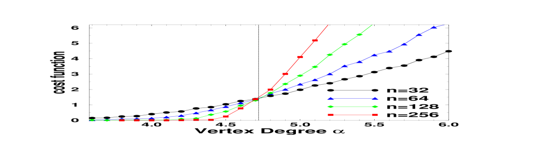
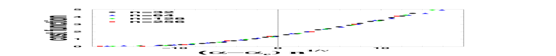
Figure 2: Plot of the average cost as a function of the average vertex degree $\alpha$ for random graph 3-coloring. According to Eq. (6), the data collapse in the insert predicts $\alpha_{\rm crit}\approx 4.72$, indicated by a vertical line.

In conclusion, we have presented a new optimization method, called extremal optimization due to its derivation from extremally driven statistical systems. At each update step, the algorithm assigns fitnesses to variables $x_{i}$, and then generates moves by randomly updating an “unfit” variable. EO gives no consideration to the move’s outcome. Large fluctuations in the cost function can accumulate over many updates; only the bias against poor fitnesses guides EO back towards improved solutions.

A drawback to EO is that a general definition of fitness for individual variables may prove ambiguous or even impossible. Also, each variable $x_{i}$ could have a large number of states to choose from, as in $K$-coloring with large $K$; random updates would then be more likely to remove than to create well-adapted variables (this is notably the case for the traveling salesman problem BoPe1 ). And in highly connected systems (e. g. for $\alpha\gg 1$ in $K$-coloring), EO may be slowed down considerably by continual fitness recalculations [step (2a)].

However, extremal optimization is readily applicable to problems whose cost can be decomposed into contributions from individual degrees of freedom. It is easily implemented and, using very few parameters, it can prove highly competitive. We have shown this on the spin glass Hamiltonian, obtaining $d=3$ and $4$ ground-state energies that are consistent with the best known results. We have also used EO to explore the phase transition in random graph 3-coloring. Its results enable us to provide, by way of finite size scaling, the first sound estimates of critical values for this problem.

- (1) P. Bak How Nature Works (Springer, New York, 1996).
- (2) E. Somfai, A Czirok, and T. Vicsek, J. Phys. A 27, L757-L763 (1994).
- (3) M. Cieplak, A. Giacometti, A. Maritan, A. Rinaldo, I. Rodriguez-Iturbe, and J. R. Banavar, J. Stat. Phys. 91, 1-15 (1998).
- (4) M. Paczuski, S. Maslov, and P. Bak, Phys. Rev. E 53, 414-443 (1996).
- (5) P. Bak and K. Sneppen, Phys. Rev. Lett. 71, 4083-4086 (1993).
- (6) S. Boettcher and M. Paczuski, Phys. Rev. E 54, 1082-1095 (1996).
- (7) P. Bak, C. Tang, and K. Wiesenfeld, Phys. Rev. Lett. 59, 381-384 (1987).
- (8) S. Boettcher and A. G. Percus, Artificial Intelligence 119, 275-286 (2000).
- (9) S. Kirkpatrick, C. D. Gelatt, and M. P. Vecchi, Science 220, 671-680 (1983).
- (10) J. Holland, Adaptation in Natural and Artificial Systems (University of Michigan Press, Ann Arbor, 1975).
- (11) J. Houdayer and O. C. Martin, Phys. Rev. Lett.83, 1030-1033 (1999).
- (12) F.-M. Dittes, Phys. Rev. Lett.76, 4651-4655 (1996).
- (13) A. Mobius, A. Neklioudov, A. DiazSanchez, K. H. Hoffmann, A. Fachat, M. Schreiber, Phys. Rev. Lett.79, 4297-4301 (1997).
- (14) K. F. Pal, Physica A 223, 283-292 (1996).
- (15) A. K. Hartmann, Europhys. Lett. 40, 429 (1997).
- (16) A. K. Hartmann, Phys. Rev. E 60, 5135-5138 (1999).
- (17) S. Boettcher, Computing in Science and Engineering 2:6, 75 (2000).
- (18) M. Mezard, G. Parisi, and M. A. Virasoro, Spin Glass Theory and Beyond (World Scientific, Singapore, 1987).
- (19) F. Barahona, J. Phys. A 15, 3241-3253 (1982).
- (20) S. Boettcher and A. G. Percus, Extremal Optimization for Graph Partitioning, (in preparation).
- (21) S. Boettcher, A. G. Percus, and M. Grigni, Lecture Notes in Computer Science 1917, 447-456 (2000).
- (22) M. R. Garey and D. S. Johnson, Computers and Intractability, A Guide to the Theory of NP-Completeness (W. H. Freeman, New York, 1979).
- (23) See Frontiers in problem solving: Phase transitions and complexity, Special issue of Artificial Intelligence 81:1–2 (1996).
- (24) J. Culberson and I. P. Gent, Frozen Development in Graph Coloring, available at http://www.apes.cs.strath.ac.uk/apesreports.html.
- (25) B. Bollobas, Random Graphs, (Academic Press, London, 1985).
- (26) P. Cheeseman, B. Kanefsky, and W. M. Taylor, Where the really hard problems are, in Proc. of IJCAI-91, eds. J. Mylopoulos and R. Rediter (Morgan Kaufmann, San Mateo, CA, 1991), 331-337.
- (27) S. Boettcher, J. Math. Phys. A 32, 5201-5211 (1999).
- (28) S. Boettcher, M. Grigni, G. Istrate, and A. G. Percus, Phase Transitions and Computational Complexity, in preparation.
- (29) R. Monasson, R. Zecchina, S. Kirkpatrick, B. Selman, and L. Troyansky, Nature 400, 133-137 (1999).
- (30) S. Kirkpatrick and B. Selman, Science 264, 1297-1301 (1994).