^∗ University of Coimbra, 3000, Coimbra, Portugal
^†Institute of Semiconductor Physics, 630090, Novosibirsk, Russia

We have developed a consistent theory of the Heisenberg quantum antiferromagnet in the disordered phase with a short range antiferromagnetic order on the basis of the path integral for spin coherent states. We have presented the Lagrangian of the theory in a form which is explicitly invariant under rotations and found natural variables in terms of which one can construct a natural perturbation theory. The short wave spin fluctuations are similar to those in the spin wave theory and they are of the order of the parameter $1/2s$ where $s$ is the spin magnitude. The long wave spin fluctuations are governed by the nonlinear sigma model and are of the order of the the parameter $1/N$, where $N$ is the number of field components. We also have shown that the short wave spin fluctuations must be evaluated accurately and the continuum limit in time of the path integral must be performed after all summation over the frequencies $\omega$. In the framework of our approach we have obtained the response function for the spin fluctuations for all region of the frequency $\omega$ and the wave vector ${\bf k}$ and have calculated the free energy of the system. We have also reproduced the known results for the spin correlation length in the lowest order in $1/N$.

Pacs: 75.50.Ee,74.20.Mn

1 Introduction

The theory of the two–dimensional Heisenberg antiferromagnet (AF) has attracted great interest during the last years in connection with the problem of AF fluctuations in the copper oxides [1, 2, 4, 3]. We especially call the attention of the reader to the review [1] in which a general situation of the quantum AF (QAF) has been elucidated. The approach of these papers was based on the sigma model, which describes the long wave fluctuations of the Heisenberg AF in the paramagnetic phase with a short range antiferromagnetic order [5]. The sigma model is the continuous model for the unit vector ${\bf n}(t,{\bf r}),\ {\bf n}^{2}=1$ in the 1 + 2 time and space dimensions [7, 8]. As a long wave theory the sigma model can make a lot of physical predictions such as the structure of the long wave fluctuations and the magnitude of the correlation length [2, 4, 6]. The basic parameters of the sigma model, the spin rigidity $\rho_{s}$, the velocity of sound $c_{s}$, and the perpendicular susceptibility $\chi_{\perp}=\rho_{s}/c_{s}^{2}$ are calculated independently in the framework of the spin wave theory [9].

The derivation of the sigma model presented in the papers [1] and [5], without taking into account fluctuations, is equivalent to the statement that the classical equations of motion for the spin fluctuations in the QAF are described by the sigma model. But up to now a consistent theory of the spin fluctuations for the QAF with short range AF order was absent. Such is precisely the topic of this paper.

Our approach to the description of the QAF is based on the functional integral for the generalized partition function (GPF) in terms of spin coherent states. This approach permits to solve some problems of the theory.

This paper contains the following basic results:

1) A method of constructing spin coherent states (Appendix A) invariant under rotations was proposed. It permits to write out the Berry phase and its generalization for the final time step the Perelomov phase [12] for the QAF in a form which is explicitly invariant under rotations. By the way the Lagrangian for QAF is explicitly invariant under rotations which permits to construct the theory of QAF with short range AF order in an invariant manner (section 2.2).

2) Variables $\Omega$ and ${\bf M},$ which describes AF and ferromagnetic spin fluctuations, have been introduced . These fields $\Omega$ and ${\bf M}$ are not free. Inded $\mbox{\boldmath{$\Omega$}}^{2}=1$ and $\mbox{\boldmath{$\Omega$}}\cdot{\bf M}=0$. We remove the first constraint with the help of the well known method of the Lagrange multiplier $\lambda$. For the elimination of the second constraint we have used the Faddev - Popov trick which previously was used in quantum electrodynamics (section 2.3).

3) We have formulated he basic $1/2s$ approximation (section 2.4) in the framework of which we have calculated the basic objects of the theory: a) the Green functions of the $\Omega$, ${\bf M}$, and $\lambda$ fields; b) the correlation length in a zero approximation; c) the spin correlation function as function of the frequency $\omega$ and the wave vector ${\bf k}$ (section 2.5)

4) In the leading approximation in $1/2s$ we have integrated the action over the ${\bf M}$ field and we have obtained (section 2.6) some sort of the quantum lattice rotator model (QLRM) [1], [2]. We shall call this model the spin–rotator model. It can be useful in the calculations in the basic $1/2s$ approximation.

5) It was demonstrated that the continuous approach in time can not be applied for calculations of the corrections to the basic approximation. The free energy also can not be calculated on the basis of the continuous approach in time. The method of calculations at the final time step was developed (section 3.1). After that we calculated the free energy (section 3.2), and the first order corrections to the basic approximation (section 3.3): the effective action, the magnon dispersion law, and the correlation length.

6) We have performed the separation of fluctuations for the $\Omega$ field by introducing some separation scale $\hbar/\xi\ll\Lambda\ll\hbar\pi/a$ in momentum space. This separation of scales was performed on the basis of the Pauli - Villars transformation. As a result, we have obtain the long wave nonlinear sigma model with additional contributions from short wave fluctuations. We presented an arguments showing that these short wave contributions can be included in the renormalization of the spin stiffness and the velocity of sound.

2 Basic continuous approximation

2.1 Magnetic fluctuations and 1/2s approximation

We consider the spin system which is described by the following Heisenberg Hamiltonian:

$$\hat{H}_{Hei}=\frac{J}{2}\sum_{l,l^{\prime}=<l>}\hat{\bf S}_{l}\cdot\hat{\bf S}_{l^{\prime}},\ \ \ \hat{\bf S}_{l}\cdot\hat{\bf S}_{l}=s(s+1),$$ (1)

where $\hat{\bf S}_{l}$ are the spin operators; the index $l$ runs over a two–dimensional square lattice; the index $l^{\prime}$ runs over the nearest neighbors of the site $l$; $J>0$ is the exchange constant which, since it is positive, corresponds to the AF spin interaction; and $s$ is the magnitude of spin. The most efficient method of dealing with a spin system is based on the representation of the GPF $Z$ or the generating functional of the spin Green functions in the form of the functional integral over spin coherent states $z,z^{*}$ [10, 11] or over the unit vector ${\bf n},\ {\bf n}^{2}=1,$ on a sphere [1]:

$$Z=Tr\left[\exp\left(-\beta\hat{H}\right)\right],\ \ \ \beta=1/T,$$ (2)

$$Z=\int_{-\infty}^{\infty}\cdots\int_{-\infty}^{\infty}D\mu({\bf n})\exp(A({\bf n})),$$ (3)

$$D\mu({\bf n})=\prod_{\tau l}\frac{2s+1}{2\pi}\delta({\bf n}_{\tau l}^{2}-1)d{\bf n}_{\tau l}$$ (4)

where $T$ is the temperature, $\tau$ is the imaginary time, and $A({\bf n})$ is the action of the system. In the continuum approximation, which is valid in leading order over $1/2s$ the expression of the action $A({\bf n})$is simplified

$$A({\bf n})=-\int_{0}^{\beta}\sum_{l}{\cal L}_{tot}(\tau,l)d\tau,\ \ \ {\cal L}_{tot}(\tau,l)={\cal L}_{kin}(\tau,l)+{\cal H}(\tau,l),$$ (5)

$${\cal L}_{kin}(\tau,l)=is(1-\cos\theta_{\tau l})\dot{\varphi}_{\tau l},\ \ \ {\cal H}(\tau,l)=\frac{Js^{2}}{2}\sum_{l^{\prime}=<l>}{\bf n}_{\tau l}\cdot{\bf n}_{\tau l^{\prime}},$$ (6)

where $\theta,\varphi$ are the Euler angles of the unit vector ${\bf n}=(\cos\varphi\sin\theta,\sin\varphi\sin\theta,\cos\theta)$, and ${\bf\dot{\bf\varphi}}_{\tau l}$ is the time derivative of this angle. The kinetic part of the action ${\cal L}_{kin}$ is highly nonlinear and it is not clear how to proceed with it consistently. Some essential steps in this direction where made in [1, 5] but they do not have a final character.

Further in this paper we use the idea of the near AF order. Following this fundamental hypothesis, we split our square lattice into two AF sublattices ${\rm a}$ and ${\rm b}$. In the sublattice ${\rm a}$ the spins ${\bf S}$ are directed along some axis ${\bf\Omega}$, in the sublattice ${\rm b}$ they are directed in the opposite direction. In this way, we obtain a new square lattice with two spins ${\rm a}$ and ${\rm b}$ in the elementary cell with a volume $2a^{2}$, where $a$ is the space distance between spins. The axes of this new lattice are rotated by 45 degrees with respect to the primary axes. We assume that this AF order is only defined locally and any global AF order is absent. As a result, the summation over the lattice sites $l$ and $l^{\prime}$ can be expressed as a summation over $l\in{\rm a}$ and $l^{\prime}\in{\rm b}$. which specify the space positions of the spins in the sublattices ${\rm a}$ and ${\rm b}$. In terms of this notation, the Lagrangian ${\cal L}_{kin}$ can be expressed as a sum of two such Lagrangians, one for the sublattice ${\rm a}$ and another for the sublattice ${\rm b}$ in terms of two vectors ${\bf n}_{a}(\tau,l)$ and ${\bf n}_{b}(\tau,l^{\prime})$. The Hamiltonian ${\cal H}$ conserves its form if $l\in{\rm a}$ and $l^{\prime}\in{\rm b}$ but $J/2\rightarrow J$ because the double summation is absent now.

In this way we have two spins in each AF elementary cell which are defined in the different space positions $l$ and $l^{\prime}$. This circumstance is not convenient for subsequent nonlinear changes of variables. One can introduce new variables ${\bf n}_{a,b}(\tau,l)$ which are both defined at the sublattice ${\rm a}$ (or at the center of the AF elementary cell).

For that we pass to the Fourier image ${\bf n}_{a,b}(\tau,{\bf k})$ of the original vectors ${\bf n}_{a}(\tau,l)$ and ${\bf n}_{b}(\tau,l^{\prime})$, where the momentum vector ${\bf k}$ runs over the AF Brillouin band. We can return to the space representation and consider the coordinate $\rho$ as continuous variable. As a result we have the following definition:

$${\bf n}_{a,b}(\tau,\mbox{\boldmath{$\rho$}})=\sqrt{1/N_{s}}\sum_{{\bf k}}\exp\left(i{\bf k}\cdot\mbox{\boldmath{$\rho$}}\right){\bf n}_{a,b}(\tau,{\bf k}),$$ (7)

where $2N_{s}$ is the total number of sites in the space lattice. Of course, we assume periodic boundary conditions. We can put the variable $\rho$ now on the sublattice ${\rm a}$ (or in a center of the AF elementary cell). One can check that the Lagrangian ${\cal L}_{kin}$ will be the same in terms of the new variables ${\bf n}_{a,b}(\tau,\mbox{\boldmath{$\rho$}})\equiv{\bf n}_{a,b}(\tau,l)$. By the same manner one can change the measure of integration (4) and write out it in terms of ${\bf n}_{a,b}(\tau,l)$. The Hamiltonian ${\cal H}$ preserves its simple form in the momentum representation.

2.2 Invariant Lagrangian

The form of the Lagrangian ${\cal L}_{kin}$ is not invariant under rotations although the physical problem itself is invariant. The reason for such situation was explained in detail in the Appendix (A.2). In the Appendix (A.3) an invariant form of the Lagrangian ${\cal L}_{kin}$ was proposed (120). For two sublattices ${\rm a}$ and ${\rm b}$ it has a form

$${\cal L}_{kin}=-is{\bf n}_{a}\cdot[{\bf m}_{a}\times\dot{\bf m}_{a}]-is{\bf n}_{b}\cdot[{\bf m}_{b}\times\dot{\bf m}_{b}].$$ (8)

Eq.(8) for ${\cal L}_{kin}$ is valid for any choice the unit vectors ${\bf m}_{a,b}$ if they satisfy conditions: ${\bf m}^{2}_{a,b}=1,\ {\bf n}_{a,b}\cdot{\bf m}_{a,b}=0$. For the problem of the quantum AF with two sublattices we can choose the following expression for vectors ${\bf m}_{a,b}$

$${\bf m}_{a}=\frac{{\bf n}_{b}-({\bf n}_{b}\cdot{\bf n}_{a}){\bf n}_{a}}{\sqrt{1-({\bf n}_{a}\cdot{\bf n}_{b})^{2}}},\ \ \ {\bf m}_{b}=\frac{{\bf n}_{a}-({\bf n}_{a}\cdot{\bf n}_{b}){\bf n}_{b}}{\sqrt{1-({\bf n}_{a}\cdot{\bf n}_{b})^{2}}}.$$ (9)

This choice means physically that the vectors ${\bf n}_{a},{\bf m}_{a}$ determines the reference frame for the sublattice ${\rm a}$, and the vectors ${\bf n}_{b},{\bf m}_{b}$ determines the reference frame for the sublattice ${\rm b}$ (see Appendix (A.3)). Substituting these expressions for ${\bf m}_{a,b}$ into Eq. (8) we get for ${\cal L}_{kin}$ an invariant over rotation form for ${\cal L}_{kin}$ and also ${\cal H}$ (see (6))

$${\cal L}_{kin}=\frac{is}{1-{\bf n}_{a\tau l}\cdot{\bf n}_{b\tau l}}(\dot{\bf n}_{a\tau l}-\dot{\bf n}_{b\tau l})\cdot[{\bf n}_{a\tau l}\times{\bf n}_{b\tau l}],\ \ \$$ (10)

$${\cal H}=Js^{2}\sum_{l^{\prime}=<l>}{\bf n}_{a\tau l}\cdot{\bf n}_{b\tau l^{\prime}},\ \ \ {\bf n}_{a\tau l}\in a,\ \ \ {\bf n}_{b\tau l}\in b.$$

Now we can introduce new more convenient variables $\mbox{\boldmath{$\Omega$}}(\tau,l)$ and ${\bf M}(\tau,l)$ which realize the stereographic mapping of a sphere:

$${\bf n}_{a,b}=\frac{\pm\mbox{\boldmath{$\Omega$}}\left(1-{\bf M}^{2}/4\right)-[\mbox{\boldmath{$\Omega$}}\times{\bf M}]}{1+{\bf M}^{2}/4},\ \ \ \mbox{\boldmath{$\Omega$}}^{2}=1,\ \ \ \mbox{\boldmath{$\Omega$}}\cdot{\bf M}=0.$$ (11)

In terms of these variables the total Lagrangian ${\cal L}_{\Omega M}={\cal L}_{kin}+{\cal H}$ has the final form

$${\cal L}_{kin}= \frac{2is\dot{\mbox{\boldmath{$\Omega$}}}\cdot{\bf M}}{1+{\bf M}^{2}/4},\ \ \ {\cal H}=Js^{2}\sum_{l^{\prime}=<l>}\{\mbox{\boldmath{$\Omega$}}\cdot\mbox{\boldmath{$\Omega$}}^{\prime}[(1-{\bf M}^{2}/4)(1-{\bf M}^{\prime 2}/4)$$

$$-{\bf M}\cdot{\bf M}^{\prime}]+\mbox{\boldmath{$\Omega$}}\cdot{\bf M}^{\prime}\ \mbox{\boldmath{$\Omega$}}^{\prime}\cdot{\bf M}\}(1+{\bf M}^{2}/4)^{-1}(1+{\bf M}^{\prime 2}/4)^{-1},$$

where $\mbox{\boldmath{$\Omega$}}\equiv\mbox{\boldmath{$\Omega$}}_{\tau l},\ \mbox{\boldmath{$\Omega$}}^{\prime}\equiv\mbox{\boldmath{$\Omega$}}_{\tau l^{\prime}},\ {\bf M}\equiv{\bf M}_{\tau l},\ {\bf M}^{\prime}\equiv{\bf M}_{\tau l^{\prime}}$. After this change of variables the measure of integration $D\mu({\bf n})$ (see (4)) passes into

$$D\mu({\bf n})=\prod_{\tau l}\frac{(2s+1)^{2}}{4\pi^{2}}\delta({\bf n}^{2}_{a\tau l}-1)\delta({\bf n}^{2}_{b\tau l}-1)d{\bf n}_{a\tau l}d{\bf n}_{b\tau l}=$$ (13)

$$=\prod_{\tau l}\frac{(2s+1)^{2}}{2\pi^{2}}\frac{1-{\bf M}^{2}/4}{(1+{\bf M}^{2}/4)^{3}}\delta\left(\mbox{\boldmath{$\Omega$}}^{2}-1\right)\delta\left(\mbox{\boldmath{$\Omega$}}\cdot{\bf M}\right)d\mbox{\boldmath{$\Omega$}}d{\bf M},$$

where the product in (13) is performed over the AF (doubled) lattice cells.

2.3 Gauge transformation

The variable $\Omega$ is responsible for the AF fluctuations and the variable ${\bf M}$ for the ferromagnetic ones. The ferromagnetic fluctuations are small according to the parameter $1/2s$ and therefore one can expand the Lagrangian ${\cal L}_{\Omega M}$ (2.2) over ${\bf M}$. The vector of the ferromagnetic fluctuations ${\bf M}$ plays the role (up to factor 2s) of the canonical momentum conjugated to the canonical coordinate $\Omega$. The term of first order in ${\bf M}$ coincides (after change of variables) with previous results Manousakis [1] and Sachdev [5].

From Eq. (2.2) one can easily extract the quadratic part in the variables $\Omega$ and ${\bf M}$ of the total lagrangian, ${\cal L}_{quad}$,

$${\cal L}_{quad}=2is({\bf M}\cdot\dot{\mbox{\boldmath{$\Omega$}}})+Js^{2}\sum_{l^{\prime}\in<l>}\left[\mbox{\boldmath{$\Omega$}}^{2}-\mbox{\boldmath{$\Omega$}}\cdot\mbox{\boldmath{$\Omega$}}^{\prime}+{\bf M}^{2}+{\bf M}\cdot{\bf M}^{\prime}\right],$$ (14)

The Lagrangian ${\cal L}_{quad}$ (14) is very simple but the measure $D\mu$ (13) is not simple due to the presence of two delta– functions. Therefore we can not simply perform the Gaussian integration over the field $\Omega$ and ${\bf M}$.

To solve this problem we shall use the method of the Lagrange multiplier together with the saddle point approximation [7, 8] to eliminate $\delta(\mbox{\boldmath{$\Omega$}}^{2}-1)$:

$$\delta(\mbox{\boldmath{$\Omega$}}^{2}-1)=(2\pi)^{-1}\int_{-\infty}^{\infty}\exp\left(A_{\lambda}\right)d\lambda,$$ (15)

$$-A_{\lambda}={\cal L}_{\lambda}=(i\lambda+c_{\mu})(\mbox{\boldmath{$\Omega$}}^{2}-1)$$

where $\lambda$ is the Lagrange multiplier, and $c_{\mu}$ is a constant which will be fixed with the help of the saddle point condition [7, 8].

To eliminate $\delta(\mbox{\boldmath{$\Omega$}}\cdot{\bf M})$ we shall use some kind of the Faddev–Popov trick which was proposed in [14]. Let us consider the integral:

$$I=\int f({\bf M})\delta(\mbox{\boldmath{$\Omega$}}\cdot{\bf M})d{\bf M},$$ (16)

and insert it in the right hand side of the identity:

$$1=(\det(\hat{B}_{gaug}))^{1/2}\int\exp\left(-\frac{1}{2}\varphi\hat{B}_{gaug}\varphi\right)d\varphi/\sqrt{2\pi},$$ (17)

where $\hat{B}_{gaug}$ is a positive number or a positive definite operator for some multi dimensional generalization. After changing the order of integration over ${\bf M}$ and $\varphi$ we can make the change of the variable ${\bf M}$: ${\bf M}\rightarrow{\bf M}-\mbox{\boldmath{$\Omega$}}\varphi$. After that, due to the delta-function, we have $\varphi=(\mbox{\boldmath{$\Omega$}}\cdot{\bf M})$ and the delta–function disappears from the integral (16):

$$I=(\det(\hat{B}_{gaug}))^{1/2}\int f({\bf M}_{tr})\exp\left(A_{gaug}\right)d{\bf M}/\sqrt{2\pi},\ \ \$$ (18)

$${\bf M}_{tr}\equiv{\bf M}-\mbox{\boldmath{$\Omega$}}(\mbox{\boldmath{$\Omega$}}\cdot{\bf M}),\ \ \ -A_{gaug}={\cal L}_{gaug}=\frac{1}{2}(\mbox{\boldmath{$\Omega$}}\cdot{\bf M})\hat{\hat{B}_{gaug}}(\mbox{\boldmath{$\Omega$}}\cdot{\bf M})$$

With the help of the identity (18) we can remove the delta–function $\delta(\mbox{\boldmath{$\Omega$}}\cdot{\bf M})$ from the measure (13). As a result we must substitute ${\bf M}\rightarrow{\bf M}_{tr}$ in the Lagrangian ${\cal L}_{\Omega M}$ (2.2) and add the gauge fixing Lagrangian ${\cal L}_{gaug}$ due to the additional exponent in (18). It is very convenient to chose the Lagrangian ${\cal L}_{gaug}$ in the form

$${\cal L}_{gaug}=Js^{2}\sum_{l^{\prime}\in<l>}\left[(\mbox{\boldmath{$\Omega$}}\cdot{\bf M})^{2}+(\mbox{\boldmath{$\Omega$}}\cdot{\bf M})(\mbox{\boldmath{$\Omega$}}^{\prime}\cdot{\bf M}^{\prime})\right].$$ (19)

Such choice kills the major dependence on $\Omega$ in the Lagrangian (14) which appears due to substitution ${\bf M}\rightarrow{\bf M}_{tr}$. We can also substitute ${\bf M}_{tr}\rightarrow{\bf M}$ in the first term of the Lagrangian ${\cal L}_{quad}$ (14) due to the identity $(\mbox{\boldmath{$\Omega$}}\cdot\dot{\mbox{\boldmath{$\Omega$}}})=0$. In this way, the expression (14) for ${\cal L}_{quad}$ is valid in the leading order with respect to $1/2s$.

The final expression for the GPF $Z$ of the Heisenberg AF is

$$Z=\int_{-\infty}^{\infty}\cdots\int_{-\infty}^{\infty}D\mu(\mbox{\boldmath{$\Omega$}},{\bf M},\lambda)\exp\left[A(\mbox{\boldmath{$\Omega$}},{\bf M},\lambda)\right],$$ (20)

$$D\mu(\mbox{\boldmath{$\Omega$}},{\bf M},\lambda)=Z_{gaug}D\mu(\mbox{\boldmath{$\Omega$}},{\bf M})D\mu(\lambda),\ \ \ Z_{gaug}=\left[\det(\hat{B}_{gaug})\right]^{1/2},$$

$$D\mu(\mbox{\boldmath{$\Omega$}},{\bf M})=\prod_{\tau l}\frac{(2s+1)^{3}(1-{\bf M}^{2}/4)}{(2\pi)^{3}(1+{\bf M}^{2}/4)^{3}}d\mbox{\boldmath{$\Omega$}}(\tau,l)d{\bf M}(\tau,l),$$

$$D\mu(\lambda)=\prod_{\tau l}\frac{2d\lambda(\tau,l)}{(2s+1)(2\pi)^{1/2}},$$

where $D\mu(\mbox{\boldmath{$\Omega$}},{\bf M},\lambda)$ is the measure of an integration, and the action $A(\mbox{\boldmath{$\Omega$}},{\bf M},\lambda)$ is determined by the total Lagrangian ${\cal L}_{tot}={\cal L}_{\Omega M}+{\cal L}_{gaug}+{\cal L}_{\lambda}$ (2.2,15,19).

2.4 Properties of the basic approximation

One can pass to the $q=(\omega,{\bf k})$ momentum representation ($\omega$ is the frequency, ${\bf k}$ is the wave vector), and write out the total quadratic part of the Lagrangian in the matrix form

$${\cal L}_{quad}(q)=s{\bf X}^{*}_{q}\hat{\Lambda}(q){\bf X}_{q},\ \ \ {\bf X}^{*}_{q}=(\mbox{\boldmath{$\Omega$}}^{*}_{q},{\bf M}^{*}_{q}),$$ (21)

$$\hat{\Lambda}(q){\bf X}_{q}=\left(\begin{array}[]{cc}P^{\prime}_{\bf k},&\omega\\ -\omega,&Q_{\bf k}\end{array}\right)\left(\begin{array}[]{c}\mbox{\boldmath{$\Omega$}}_{q}\\ {\bf M}_{q}\end{array}\right),\ \ \ P^{\prime}_{\bf k}=P_{\bf k}+c_{\mu},\ \ \ c_{\mu}=\mu_{0}^{2}/2{\cal J},$$ (26)

$$(Q_{\bf k},P_{\bf k})={\cal J}(1\pm\gamma_{\bf k}),\ \ \ \gamma_{\bf k}=(1/2)(\cos(k_{x}a)+\cos(k_{y}a)),\ \ \ {\cal J}=Jsz.$$

Here ${\bf X}_{q}$ is a two component vector field which combines the vector fields $\mbox{\boldmath{$\Omega$}}_{q}$ and ${\bf M}_{q}$; the constant $c_{\mu}$ (15) is expressed through the constant $\mu_{0}$ which is the mass of the $\Omega$ field in the lowest order of perturbation theory. One can invert the $2\times 2$ matrix $\hat{\Lambda}(q)$ and get the bare Green function $\hat{G}_{q}$ of the $\mbox{\boldmath{$\Omega$}}_{q}$ and ${\bf M}_{q}$ fields

$$\hat{G}_{q}\equiv\left(\begin{array}[]{cc}G^{\Omega}_{q},&G^{d}_{q}\\ G_{q}^{u},&G^{M}_{q}\end{array}\right)=\frac{1}{2s}\left(\hat{\Lambda}(q)\right)^{-1}=\frac{1}{2sL_{q}}\left(\begin{array}[]{cc}Q_{\bf k},&-\omega\\ \omega,&P^{\prime}_{\bf k}\end{array}\right),$$ (31)

$$L_{q}=\omega^{2}+\omega^{2}_{0{\bf k}},\ \ \ \omega^{2}_{0{\bf k}}=P^{\prime}_{\bf k}Q_{\bf k}=(1-\gamma^{2}_{\bf k}){\cal J}^{2}+(1+\gamma_{\bf k})\mu_{0}^{2}/2.$$

Here $\omega_{0{\bf k}}$ is the primary magnon frequency in the paramagnetic phase, $G^{\Omega}_{q},\ G^{d}_{q},\ G_{q}^{u},\ G^{M}_{q}$ are notations for the matrix elements of the matrix Green function $\hat{G}_{q}$.

At first let us discuss the parameter of the perturbation theory. One can see from an explicit form of the Lagrangian (2.2) that the spin wave nonlinearity of the theory is caused by the term ${\bf M}_{tr}$ and its modifications. Its average value is

$$<{\bf M}^{2}_{tr}>=(N-1)\sum_{q}G^{M}_{q}=\frac{(N-1)T}{2s}\sum_{\omega=2\pi nT,{\bf k}}\frac{P_{\bf k}}{\omega^{2}+\omega^{2}_{0{\bf k}}},$$ (32)

where $N=3$ is the number of components of the $\Omega$ field. Summation over $\omega$ is obtained by standard methods [8] and we have

$$<{\bf M}^{2}_{tr}>=\frac{(N-1)}{2s}\sum_{\bf k}\frac{P_{\bf k}}{2\omega_{0{\bf k}}}(1+2n_{0{\bf k}})=\frac{(N-1)}{4s}\left\{\begin{array}[]{cc}C_{M0},&T\ll{\cal J}\\ (T/{\cal J})C_{M\infty},&T\gg{\cal J},\end{array}\right..$$ (35)

Here, $N=3$ is the number of components of fields ${\bf M}$ and $\Omega$, $n_{0{\bf k}}=\left(\exp(\omega_{0{\bf k}}/T)-1\right)^{-1}$ is the Plank function, and summation over ${\bf k}$ means the normalized integration over the AF Brillouin band:

$$\sum_{\bf k}f({\bf k})\equiv\int\frac{a^{2}d{\bf k}}{2\pi^{2}}f({\bf k}).$$ (36)

The constants $C_{M0}$ and $C_{M\infty}$ are defined by the relations

$$C_{M0}=\sum_{\bf k}\sqrt{\frac{1-\gamma_{\bf k}}{1+\gamma_{\bf k}}}=c_{0}-c_{1}=0.65075,\ \ \ C_{M\infty}=\sum_{\bf k}\frac{2}{1+\gamma_{\bf k}}=1.48491,$$ (37)

where all sum of the type of (36) are calculated by the following method

$$\sum_{\bf k}f(\gamma_{\bf k})=\int_{0}^{1}f(\epsilon)\rho(\epsilon)d\epsilon,\ \ \ c_{n}=\sum_{\bf k}\frac{\gamma^{n}_{\bf k}}{\sqrt{1-\gamma^{2}_{\bf k}}},$$ (38)

$$\rho(\epsilon)=\sum_{\bf k}\delta(\epsilon-\gamma_{\bf k})=\frac{4}{\pi^{2}}K(1-\epsilon^{2}),$$

where $K(x)$ is the complete elliptic integral of the first kind. By the same manner one can calculate the different time and space average

$$<M_{i}(\tau+\delta,{\bf l}+{\bf r})\Omega_{j}(\tau,{\bf l})>=\delta_{ij}\frac{T}{2s}\sum_{\omega=2\pi nT,{\bf k}}e^{i\delta\tau+i{\bf k}\cdot{\bf r}}\frac{\omega}{\omega^{2}+\omega^{2}_{0{\bf k}}}=$$ (39)

$$=\frac{i}{4s}\delta_{ij}\epsilon(\delta)\sum_{\bf k}\frac{\exp(i{\bf k}\cdot{\bf r}-|\delta|\omega_{0{\bf k}})}{1-\exp(-\beta\omega_{0{\bf k}})}.$$

Here $\epsilon(\delta)$ is the sign function: $\epsilon(\delta)=1$ for $\delta>0$, $\epsilon(\delta)=-1$ for $\delta<0$. For ${\bf r}=0$ and $\delta{\cal J}\ll 1$ we have an explicit expression

$$<M_{i}(\tau+\delta,{\bf l})\Omega_{j}(\tau,{\bf l})>=\frac{i}{4s}\delta_{ij}\epsilon(\delta)\left\{\begin{array}[]{cc}1,&T\ll{\cal J}\\ (T/{\cal J})c_{0},&T\gg{\cal J},\end{array}\right..$$ (42)

From Eqs. (35,39) we clearly see that the parameter of perturbation theory is $1/2s$ at low temperatures $T\ll{\cal J}$ and $T/(2s{\cal J})$ at high temperatures $T\geq{\cal J}$. Thus, perturbation theory is working when $1/2s$ is a small parameter and the temperature is not high. We remind the reader that this is just the applicability condition of the spin wave theory.

Now we can consider the saddle point condition for the $\lambda$ field $<\mbox{\boldmath{$\Omega$}}^{2}>=1$ which is the most important constraint of the theory which determines its phase state:

$$1=<\mbox{\boldmath{$\Omega$}}^{2}>=N\sum_{q}G^{\Omega}_{q}=\frac{NT}{2s}\sum_{\omega=2\pi nT}\sum_{\bf k}\frac{Q_{\bf k}}{\omega^{2}+\omega^{2}_{0{\bf k}}},$$ (43)

$$1=<\mbox{\boldmath{$\Omega$}}^{2}>=\frac{N}{2s}\sum_{\bf k}\frac{Q_{\bf k}}{2\omega_{0{\bf k}}}(1+2n_{0{\bf k}}),$$ (44)

The right hand side of Eq. (44) contains two terms. The first term $Q_{\bf k}/2\omega_{0{\bf k}}$ is responsible for the quantum fluctuations of the $\Omega$ field.The second term $Q_{\bf k}n_{0{\bf k}}/\omega_{0{\bf k}}$ is responsible for the classical thermal fluctuations of the $\Omega$ field. The role of these two terms is quite different. The quantum fluctuations are small with respect to the parameter of perturbation theory $1/2s$ and for basic approximation they can be neglected. The quantum fluctuation can be considered in the continuum approximation for which $Q_{\bf k}\simeq 2{\cal J}$ and $\omega^{2}_{0{\bf k}}\simeq c^{2}_{0s}{\bf k}^{2}+\mu^{2}$, where $c_{0s}$ is the primary velocity of sound and $c^{2}_{0s}=2J^{2}s^{2}za^{2}/\hbar^{2}$. The integration over the two dimensional momentum ${\bf k}$ can be easily performed [4]). The integration over the angle is trivial, and integration over the modulus $|{\bf k}|$ is performed if we introduce new variable of integration $x=\beta\omega_{0{\bf k}}$. As a result we have the constraint condition

$$1=-\frac{TN}{2\pi Js^{2}}\ln(1-\exp(-\mu/T))\simeq-\frac{TN}{2\pi Js^{2}}\ln(\mu/T)).$$ (45)

The coefficient before the logarithm in this equation is always small when the regime of the weak coupling is valid. At small temperatures $T\ll{\cal J}$ this is obvious. At the temperature $T\simeq{\cal J}$ this coefficient coincides with the parameter of perturbation theory (35) and also must be considered as small. This means the logarithm in (45) must be negative and large in modulus. This leads to the condition $\mu/T\ll 1$ which justifies the last simplification in (45). As a result we have the well known [1, 2, 4] zero order expression for $\mu$

$$\mu=T\exp\left(-\frac{2\pi Js^{2}}{TN}\right),\ \ \ \xi=\hbar c_{s}/\mu,$$ (46)

where $\xi$ is the correlation length. From Eq. (46), the very important conclusion follows: in the regime of the weak coupling the correlation length $\xi$ is much larger than the lattice constant $a$. This conclusion makes possible the scale separation for the problem of disordered QAF [2].

To close the theory it is helpful to define the polarization operator $\Pi(q)$ of the $\Omega$ field

$$A_{\lambda quad}=-\frac{1}{2}\sum_{q}\lambda^{*}(q)\Pi(q)\lambda(q),$$ (47)

which is simply a loop, and the Green function of the $\lambda$ field is $\Pi(q)^{-1}$. In the lowest approximation $\Pi(q)$ is simply a loop from two Green function $G^{\Omega}$

$$\Pi_{0}(q)=2NT\sum_{q^{\prime}}G^{\Omega}(q^{\prime})G^{\Omega}(q-q^{\prime}).$$ (48)

Using the Green function $G^{\Omega}(q)$ from (31) we can perform the summation over $\omega$ and have the expression for the simple loop

$$\Pi_{0}(q)=\frac{N}{4s^{2}}\sum_{\bf k^{\prime}}(1+2n_{1})\frac{Q_{1}Q_{2}}{\omega_{1}\omega_{2}}\left[\frac{\omega_{2}+\omega_{1}}{\omega^{2}+(\omega_{2}+\omega_{1})^{2}}+\frac{\omega_{2}-\omega_{1}}{\omega^{2}+(\omega_{2}-\omega_{1})^{2}}\right],$$ (49)

where the index $i:=1,2$ corresponds the momentum ${\bf k}_{1}\equiv{\bf k}^{\prime}$ and ${\bf k}_{2}\equiv{\bf k}-{\bf k}^{\prime}$. The main contribution in $1/2s$ in (49) is from the thermal fluctuations even at low temperatures $T$, because the integral strength of such fluctuations is fixed by the saddle point condition (43) and does not depend on temperature. The explicit form for $\Pi_{0}(q)$ may be obtained in two limiting cases $\hbar q\gg T$ and $\hbar q\ll T$, where $q^{2}=\omega^{2}+c^{2}_{s}k^{2}$. In the first case the momentum $k^{\prime}\sim T/c_{s}\ll q$, and we can separate the integration over ${\bf k}^{\prime}$ and put ${\bf k}^{\prime}=0$ in all places in (49) affected by the factor $n_{1}\equiv n({\bf k}^{\prime})$. The result is extremely simple

$$\Pi_{0}(q)=4G^{\Omega}(q)=\frac{2{\cal J}(1+\gamma_{\bf k})}{s(\omega^{2}+\omega^{2}_{0{\bf k}})},\ \ \ q\gg k_{T},\ \ \ k_{T}=T/c_{s}.$$ (50)

At small $q\ll c_{s}/a$ a similar result was obtained in [4]. Notice, that it exceeds the quantum contribution in (49) $\Pi_{0}(q)=N/4q$ in the large parameter $16s{\cal J}/Nq$. The second limiting case $\hbar q\ll T$ lies in the purely continuum region. It corresponds to pure classical two dimensional case: $\omega=0$, and $\omega^{\prime}=0$. Integration over ${\bf k}^{\prime}$ can be easily performed, the result coincides with [4] up to the normalization factor:

$$\Pi_{0}(k)=\frac{8NT}{\pi s^{2}q\sqrt{q^{2}+4\mu^{2}}}\ln\left(\frac{q+\sqrt{q^{2}+4\mu^{2}}}{2\mu}\right),\ \ \ q=c_{s}k.$$ (51)

2.5 The spin correlation functions

The approach of this paper allows us to find the spin correlation functions in all values of $\omega$ and ${\bf k}$. The dynamical spin susceptibility is determined by the relation

$$\chi(\omega,{\bf k})\delta_{ij}=-\frac{i}{\hbar}\int_{0}^{\infty}d\tau\sum_{\bf l}Tr\left\{\left[\hat{S}_{i}(\tau,{\bf l}),\hat{S}_{j}(0,{\bf 0})\right]\right.\cdot$$ (52)

$$\cdot\left.\exp\left(\beta(F-\hat{H})\right)\right\}\exp\left(i\omega\tau-ia{\bf k}\cdot{\bf l}\right),$$

where $F=-T\ln(Z)$ is the free energy, and the wave vector ${\bf k}$ runs without limitations over the Brillouin band. It is well known that the dynamical spin susceptibility $\chi(\omega,{\bf k})$ coincides with the temperature Green function continued on the imaginary frequency $\omega$. It can be calculated on the basis of the functional integral (20)

$$\chi(\omega,{\bf k})\delta_{ij}\delta({\omega-\omega^{\prime}})\delta({{\bf k}-{\bf k}^{\prime}})=-\frac{is^{2}}{\hbar}<n^{*}_{i}(\mbox{\boldmath{$\Omega$}},{\bf M},\omega^{\prime},{\bf k}^{\prime})n_{j}(\mbox{\boldmath{$\Omega$}},{\bf M},\omega,{\bf k})>,$$ (53)

Here, the unit vector ${\bf n}(\mbox{\boldmath{$\Omega$}},{\bf M},\omega,{\bf k})$ is a function of the fields $\mbox{\boldmath{$\Omega$}}(\tau,l),{\bf M}(\tau,l)$ according to (11); the brackets $<...>$ mean averaging over the $\mbox{\boldmath{$\Omega$}}(\tau,l),{\bf M}(\tau,l)$ fields according to (20). Eq. (53) reduces the problem of calculation of the spin Green function to the problem of the calculation of the averages of the $\Omega$ and ${\bf M}$ fields. In the lowest order in $1/2s$ it is sufficient to use the lowest order relation

$${\bf n}(\mbox{\boldmath{$\Omega$}}(\tau,l),{\bf M}(\tau,l),\tau,l)\simeq e^{ia{\bf l}\cdot{\bf q}_{AF}}\mbox{\boldmath{$\Omega$}}(\tau,l)-[\mbox{\boldmath{$\Omega$}}(\tau,l)\times{\bf M}(\tau,l)],$$ (54)

where ${\bf q}_{AF}=(\pi/a,\pi/a)$ is the AF vector (11). Substituting the vector ${\bf n}$ from (54) into (53) we get the dynamical spin susceptibility as a sum of two terms $\chi(\omega,{\bf k})=\chi_{A}(\omega,{\bf k})+\chi_{F}(\omega,{\bf k})$. The spin susceptibility $\chi_{A}(\omega,{\bf k})$ is responsible for the AF fluctuations. It is proportional to the Green function $G^{\Omega}_{q}$ analytically continued and shifted by the AF vector ${\bf q}_{AF}$

$$\chi_{A}(\omega,{\bf k})=-\frac{Js^{2}z(1+\gamma_{{\bf k}^{*}})}{2(\omega^{2}-\omega^{2}_{0{\bf k}^{*}}+i\omega\delta)},$$ (55)

where ${\bf k}^{*}={\bf k}-{\bf q}_{AF}$, $\omega^{2}_{0{\bf k}}$ is the magnon frequency (31). For the spin susceptibility $\chi_{A}(\omega,{\bf k})$ we have a loop expression

$$\chi_{F}(\omega,{\bf k})=2s^{2}\sum_{q^{\prime}}\left[G^{\Omega}(q^{\prime})G^{M}(q-q^{\prime})-G^{u}(q^{\prime})G^{d}(q-q^{\prime})\right].$$ (56)

In the main approximation in $1/2s$ the first term gives the main contribution in the same manner as in (48) when the contribution from the Plank function $n_{1}$ was dominated

$$\chi_{F}(\omega,{\bf k})\simeq-\sum_{\bf k^{\prime}}n_{1}\frac{Q_{1}P^{\prime}_{2}}{2\omega_{1}\omega_{2}}\left[\frac{\omega_{2}+\omega_{1}}{\omega^{2}-(\omega_{2}+\omega_{1})^{2}+i\omega\delta}+\frac{\omega_{2}-\omega_{1}}{\omega^{2}-(\omega_{2}-\omega_{1})^{2}+i\omega\delta}\right],$$ (57)

where the notation is the same as in (48). In the case of $q=\sqrt{\omega^{2}-c^{2}_{s}k^{2}}\gg k_{T}$ the expression (57) is substantially simplified on the basis of the idea of dominant small $k^{\prime}\simeq k_{T}$,

$$\chi_{F}(\omega,{\bf k})\simeq-\frac{2s^{2}}{N}G^{M}(q)=-\frac{Js^{2}z(1-\gamma_{\bf k})}{N(\omega^{2}-\omega^{2}_{0{\bf k}}+i\omega\delta)}.$$ (58)

For the case $q\leq k_{T}$ the expression for $\chi_{F}(\omega,{\bf k})$ is not so simple and we present the result the limit $\mu\ll\omega,\ \omega_{\bf k}\ll k_{T}$

$$\chi_{F}(\omega,{\bf k})=-\frac{a^{2}T^{2}}{\pi c_{s}^{2}q}\xi(2)+i\epsilon(\omega)\frac{a^{2}T}{16\pi c_{s}^{2}|q|^{2}}\cdot$$ (59)

$$\cdot\left(2\pi\theta(q^{2})\omega(4\omega-3|q|)+\theta(-q^{2})T|q|\xi(2)\right),$$

where $\xi(n)$ is the Riemann zeta function, and $\epsilon(\omega)$ is the sign function. The two terms in (59) which are proportional to $\xi(2)$ are generated by the integral which is cut at large $k$ by the Plank distribution function $n({\bf k}^{\prime})$. The ferromagnetic spin susceptibility (60) is suppressed in comparison with the antiferromagnetic one (55) by the parameter $(qa)^{2}$.

2.6 The spin-rotator model

In the basic approximation in $1/2s$ the Lagrangian is quadratic in the ${\bf M}$ field and one can integrate over the field ${\bf M}$ and obtain the final action for the field $\Omega$ and the Lagrange multiplier $\lambda$:

$${\cal L}_{\Omega\lambda}=s(\dot{\mbox{\boldmath{$\Omega$}}}\hat{Q}^{-1}\dot{\mbox{\boldmath{$\Omega$}}})+s(\mbox{\boldmath{$\Omega$}}\hat{P}^{\prime}\mbox{\boldmath{$\Omega$}})++i\lambda\left(\mbox{\boldmath{$\Omega$}}^{2}-1\right),$$ (60)

where the quantities $\hat{Q}$ and $\hat{P}^{\prime}$ are defined in the ${\bf k}$ representation in (31). As a result of such integration the ${\bf M}$ field is a function of the $\Omega$ field: ${\bf M}=\hat{Q}^{-1}\dot{\mbox{\boldmath{$\Omega$}}}$. One can easily recognize in (32) the Lagrangian of some kind of the Quantum Lattice Rotator Model (QLRM)[2]. However it is different from the standard model due to the momentum dependence of the kinetic term in Eq. (32). We shall call such kind of models spin–rotator (SR) models. The SR model describes a quantum antiferromagnet in the limit $s\rightarrow\infty$. The QLRM is also well defined and does not contain any divergences. It allows to perform all calculations accurately because all physical quantities are well defined in the framework of this model.

3 Beyond the continuum approximation in time

3.1 Basic approach

When we try to construct the perturbation corrections to the basic approach discussed in the previous section we meet a fundamental difficulty: the integrals arising from the Green functions (31), over the frequency $\omega$, are not well defined. This is obvious from the consideration of the average $<M_{i}(\tau+\delta,{\bf l})\Omega_{j}(\tau,{\bf l})>$. The result essentially depends on the time shift $\delta$ (39) which reflects the phase space nature of the $\Omega$ and ${\bf M}$ variables: the Green functions $G^{u,d}(q)\sim\omega^{-1}$ at large $\omega$. Moreover there are some doubts that the quantity $<{\bf M}^{2}_{tr}>$ was calculated completely correctly. Actually, at low temperature

$$<{\bf M}^{2}_{tr}>\sim\sum_{\bf k}\int_{-\pi/\Delta}^{\pi/\Delta}\frac{d\omega}{2\pi}\frac{{\cal J}(1-\gamma_{\bf k})}{\omega^{2}+\omega^{2}_{0{\bf k}}}=C_{M0},$$ (61)

where $\Delta$ is the time step in the accurate definition of the GPF presented in the Appendix A (99), the interval $(-\pi/\Delta,\pi/\Delta)$ gives the one dimensional Brillouin band for the final time step $\Delta$. The limit $\Delta\rightarrow 0$ gives a correct value of this average. At first sight this limit is trivial because the integral over $\omega$ in (61) is well defined. Suppose that we were not so accurate and the numerator of (61) in fact contains a small corrections ${\cal J}(1-\gamma_{\bf k})\Rightarrow{\cal J}(1-\gamma_{\bf k})+\Delta\omega^{2}$. If now we at first calculate the integral (61) with this numerator and after that pass to the limit $\Delta\rightarrow 0$ the result will be different: $C_{M0}\rightarrow C_{M0}+1$. This example should convinced the reader that for a spin system the continuum limit of the path integral for the GPS (2-4) must be produced with sufficient accuracy: at first it is necessary to formulate the theory at finite $\Delta$ and one can put $\Delta=0$ only after the calculation of all integrals over $\omega$ has been done. Notice also that the accurate version, discrete in time, of the GPS (2-4) is necessary when we calculate the free energy.

Now, on the basis of the results of the Appendix A we get an accurate expression for the quadratic part of the action. Instead of the expression (5) for the action $A({\bf n})$ we shall use a more accurate expression

$$A({\bf n})=-\sum_{j=0}^{N_{\tau}}\sum_{l}\Delta\left[{\cal L}_{kin}(j,l)+{\cal H}(j,l)\right],$$ (62)

where $\tau=j\Delta$, and $\Delta N_{\tau}=\beta$. According to the results of the Appendix A, ${\cal L}_{kin}(j,l)$ consist of two parts ${\cal L}_{kin}={\cal L}_{mod}+{\cal L}_{pha}$. The first term is pure real the second term is pure imaginary.

According to Eq. (115) the Lagrangian ${\cal L}_{mod}$ can presented for two sublattices ${\rm a}$ and ${\rm b}$ in the form

$$\Delta{\cal L}_{mod}=-s\ln\left[(1+\underline{\bf n}_{a}\cdot{\bf n}_{a})(1+\underline{\bf n}_{b}\cdot{\bf n}_{b})/4\right],$$ (63)

where ${\bf n}_{a}={\bf n}_{a}(j,l)$, $\underline{\bf n}_{a}={\bf n}_{a}(j+1,l)$, $\underline{\bf n}_{b}={\bf n}_{b}(j+1,l)$, ${\bf n}_{b}={\bf n}_{b}(j,l)$. It is assumed that vectors $\underline{\bf n}_{a},\ {\bf n}_{a},\ \underline{\bf n}_{b},\ {\bf n}_{b}$ are functions of the dynamical variables $\Omega$ and ${\bf M}$ according to Eq. (11).

The Lagrangian ${\cal L}_{pha}$ is not so simple and according to Appendix A (123) it is

$$\Delta{\cal L}_{pha}=-\frac{s}{2}\ln\left(\frac{T_{a}\underline{T}_{a}^{*}T_{b}\underline{T}_{b}^{*}}{T_{a}^{*}\underline{T}_{a}T_{b}^{*}\underline{T}_{b}}\right),$$ (64)

where the quantity $T_{a,b}$ is defined in (125) and has a rather complicated form. The expansion of $\Delta{\cal L}_{pha}$ over the field ${\bf M}$ contains only odd powers of ${\bf M}$.

The Hamiltonian ${\cal H}({\bf n})$ can be obtained on the basis of Eq.(112) for the matrix element of the spin operator ${\bf S}$ if we substitute them in the Heisenberg Hamiltonian

$${\cal H}({\bf n})=Js^{2}\sum_{l^{\prime}\in<l>}\mbox{\boldmath{${\cal S}$}}(\underline{\bf n},{\bf n})\cdot\mbox{\boldmath{${\cal S}$}}(\underline{\bf n}^{\prime},{\bf n}^{\prime}),$$ (65)

where $\underline{\bf n}={\bf n}_{a}(j+1,l)$, ${\bf n}={\bf n}_{a}(j,l)$, $\underline{\bf n}^{\prime}={\bf n}_{b}(j+1,l^{\prime})$, ${\bf n}^{\prime}={\bf n}_{b}(j,l^{\prime})$. All these vectors are also the functions of the dynamical variables $\Omega$ and ${\bf M}$ according to Eq. (11). The vector $\mbox{\boldmath{${\cal S}$}}(\underline{\bf n},{\bf n})$ is determined by the relation

$$\mbox{\boldmath{${\cal S}$}}(\underline{\bf n},{\bf n})=\frac{<\underline{\bf n}|\hat{\bf S}|{\bf n}>}{<\underline{\bf n}|{\bf n}>}=\frac{\underline{\bf n}+{\bf n}-i[\underline{\bf n}\times{\bf n}]}{1+\underline{\bf n}\cdot{\bf n}},$$ (66)

and it transforms as a vector under rotations according to the discussion in Appendix A.

Expanding the Lagrangians ${\cal L}_{mod}$ (63), ${\cal L}_{pha}$ (64), and the Hamiltonian (65) in powers of the vector ${\bf M}$ up to second order we get

$$\Delta{\cal L}_{kin}=s[1-\underline{\mbox{\boldmath{$\Omega$}}}\cdot\mbox{\boldmath{$\Omega$}}+{\bf M}^{2}-\underline{\bf M}\cdot{\bf M}+i(\underline{\mbox{\boldmath{$\Omega$}}}\cdot{\bf M}-\mbox{\boldmath{$\Omega$}}\cdot\underline{\bf M})],\ \ \$$ (67)

$${\cal H}=Js^{2}\sum_{l^{\prime}\in<l>}[\underline{\mbox{\boldmath{$\Omega$}}}\cdot\mbox{\boldmath{$\Omega$}}-\mbox{\boldmath{$\Omega$}}\cdot\mbox{\boldmath{$\Omega$}}^{\prime}+\underline{\bf M}\cdot{\bf M}+{\bf M}\cdot{\bf M}^{\prime}-i(\underline{\mbox{\boldmath{$\Omega$}}}\cdot{\bf M}-\mbox{\boldmath{$\Omega$}}\cdot\underline{\bf M})],$$

where the usual quantities $\Omega$ and ${\bf M}$ are for the arguments $j,l$; the underlined ones are for $j+1,l$; with prime are for $j,l^{\prime}$; the underlined with prime are for $j+1,l^{\prime}$.

According to the analysis performed in the section (2.3) it is necessary to add to the Lagrangian (67) the gauge Lagrangian ${\cal L}_{gaug}$ generalizing (19) in the case of finite time step

$$\Delta{\cal L}_{gaug}=s\left[(\mbox{\boldmath{$\Omega$}}\cdot{\bf M})^{2}-(\underline{\mbox{\boldmath{$\Omega$}}}\cdot\underline{\bf M})(\mbox{\boldmath{$\Omega$}}\cdot{\bf M})\right]+$$ (68)

$$+\Delta Js^{2}\sum_{l^{\prime}\in<l>}\left[(\underline{\mbox{\boldmath{$\Omega$}}}\cdot\underline{\bf M})(\mbox{\boldmath{$\Omega$}}\cdot{\bf M})+(\mbox{\boldmath{$\Omega$}}\cdot{\bf M})(\mbox{\boldmath{$\Omega$}}^{\prime}\cdot{\bf M}^{\prime})\right].$$

This Lagrangian ${\cal L}_{gaug}$ kills the most strong interaction between the $\Omega$ and ${\bf M}$ fields.

In this step we can pass to the $q=(\omega,{\bf k})$ representation

$${\bf X}(q))=\sqrt{2/N_{t}}\sum_{j,l}e^{ia{\bf k}\cdot{\bf l}-i\Delta\omega j}{\bf X}(j,l),\ \ \ N_{t}=N_{\tau}N_{s}$$ (69)

$$\omega:=2\pi Tj,\ (-N_{\tau}+1)/2<j<(N_{\tau}-1)/2,\ \ \$$

$${\bf k}=\left(\frac{2\pi m_{a}}{bN_{a}},\frac{2\pi m_{b}}{bN_{b}}\right),\ \ \ -\frac{N_{a,b}-1}{2}<m_{a,b}<\frac{N_{a,b}-1}{2},$$

where we choose $N_{\tau},N_{a},N_{b}$ as odd numbers, $N_{s}=N_{a}N_{b}$ is the number of sites on one sublattice, $j,m_{a},m_{b}$ are natural numbers.

Now one can write the action in the form $A(\mbox{\boldmath{$\Omega$}},{\bf M})=\sum_{q}{\cal L}_{quad}(q)$ where the Lagrangian ${\cal L}_{quad}(q)$ is presented in (21) but the matrix $\hat{\Lambda}(q)$ acting on ${\bf X}_{q}=(\mbox{\boldmath{$\Omega$}}_{q},{\bf M}_{q})$ is now different

$$\hat{\Lambda}(q)=\left(\begin{array}[]{cc}\Lambda^{\Omega}(q),&\Lambda^{u}(q)\\ -\Lambda^{u}(q),&\Lambda^{M}(q)\end{array}\right),\ \ \ \Lambda^{M}(q)=1-c_{\omega}+\Delta{\cal J}(c_{\omega}+\gamma_{\bf k}),\ \ \$$ (72)

$$\Lambda^{\Omega}(q)=1-c_{\omega}+\Delta{\cal J}(c_{\omega}-\gamma_{\bf k})+\Delta\mu_{0}^{2}/2{\cal J},\ \ \ \Lambda^{u}(q)=s_{\omega}(1-\Delta{\cal J})$$

where $c_{\omega}=\cos(\omega\Delta)$ and $s_{\omega}=\sin(\omega\Delta)$. Inverting the matrix $\hat{\Lambda}(q)$ we get the Green function generalizing (31) in the case of finite time step $\Delta$

$$\hat{G}_{q}=\left(\hat{\Lambda}(q)\right)^{-1}=\frac{1}{2s\bar{L}(q)}\left(\begin{array}[]{cc}\Lambda^{M}(q),&-\Lambda^{u}(q)\\ \Lambda^{u}(q),&\Lambda^{\Omega}(q)\end{array}\right),$$ (75)

$$\bar{L}(q)\simeq(1-\Delta{\cal J}+\Delta\mu_{0}^{2}/4{\cal J})[2(1-c_{\omega})+\Delta^{2}\omega^{2}_{0{\bf k}}],$$

where the quantity $Q_{\bf k}$, $P^{\prime}_{\bf k}$, and the bare frequency $\omega_{0{\bf k}}$ were defined in (31). At small $\omega$ when $\omega\Delta\ll 1$ if we neglect small terms of order $\Delta{\cal J}$ and $\Delta\mu^{2}_{0}/{\cal J}$ the matrices $\hat{\Lambda}(q)$ and $\hat{G}_{q}$ pass (up to normalization factor $\Delta$ and $\Delta^{-1}$) into their continuum analogues (21) and (31).

Of course, the difference between the continuum expressions (21) and (31) for $\hat{\Lambda}(q)$ and $\hat{G}_{q}$ and the precise values (72) and (75) are only essential for the intermediate steps of the calculations. We want to stress that the amplitudes of the magnon scattering in the skeleton approximation are determined by the continuum action (20) and the continuum Green function (31) only.

At first we demonstrate that the simple averages calculated in the section (2.4) in fact were not calculated with sufficient accuracy. The tricks necessary to carry out the calculation are discussed in the Appendices. The result at low $T\ll{\cal J}$ are presented below.

$$<M_{i}M_{j}>=\frac{1}{4s}\delta_{ij}(1+c_{0}-c_{1}),\hskip 28.45274pt<\underline{M}_{i}M_{j}>=\frac{1}{4s}\delta_{ij}(c_{0}-c_{1}),$$ (76)

$$<M^{\prime}_{i}M_{j}>=\frac{1}{4s}\delta_{ij}(\frac{4}{\pi^{2}}+c_{1}-c_{2}),\hskip 28.45274pt<\underline{M}_{i}M^{\prime}_{j}>=\frac{1}{4s}\delta_{ij}(c_{1}-c_{2}),$$

$$<\Omega_{i}\underline{M}_{j}>=i\frac{1}{4s}\delta_{ij},\hskip 85.35826pt<\underline{\Omega}_{i}M_{j}>=-i\frac{1}{4s}\delta_{ij}$$

$$<\Omega^{\prime}_{i}\underline{M}_{j}>=i\frac{1}{\pi^{2}s}\delta_{ij},\hskip 85.35826pt<\underline{\Omega}_{i}M^{\prime}_{j}>=-i\frac{1}{\pi^{2}s}\delta_{ij},$$

$$<\Omega^{\prime}_{i}\Omega_{j}>=\frac{1}{N}\delta_{ij}(1-\frac{N}{4s}(1-\frac{4}{\pi^{2}}+c_{0}-c_{2})),\ \ \ <\underline{\Omega}_{i}\Omega_{j}>=\frac{1}{N}\delta_{ij}(1-\frac{N}{4s}),$$

$$<\Omega^{\prime}_{i}\underline{\Omega}_{j}>=\frac{1}{N}\delta_{ij}(1-\frac{N}{4s}(1+c_{0}-c_{2})),\hskip 56.9055pt<\Omega_{i}\Omega_{j}>=\frac{1}{N}\delta_{ij},$$

This calculation was performed with formulae similar to (32,39,43), but the expression (75) was used for the Green function $\hat{G}$, and summation over $\omega$ was restricted by $N_{\tau}$ terms (128). Notice, that the presence of the member $1-c_{\omega}$ in the numerator of the Green function (75) leads to the difference of the underlined and not underlined averages. This difference is caused by the contribution of large $\omega\sim\pi/\Delta$. In particularly the average $<{\bf M}^{2}_{tr}>$ calculated in (35) in fact coincides with the average $<\underline{\bf M}_{tr}\cdot{\bf M}_{tr}>$ but the actual value of $<{\bf M}^{2}_{tr}>$ is different and differs from the result of (35) on the constant $(N-1)/4s$.

3.2 Free energy

After the formulation of the theory for the finite time step $\Delta$ one can calculate the GPF and the free energy of the QAF in the paramagnetic phase. We can perform the calculation in the basic $1/2s$ approximation. The free energy has three contributions as it follows from Eq. (20) for the GPF $Z$

$$F_{AF}=-T\ln(Z)=F_{\Omega M}+F_{\lambda}+F_{gaug}.$$ (77)

In the lowest approximation in $1/2s$, $Z_{\Omega M}$, $Z_{\lambda}$, and $Z_{gaug}$ are powers of determinants. The explicit form of these determinants follows from (67,72,68), and (47,48)

$$F_{\Omega M}=\frac{TNN_{s}}{2}\sum_{\omega{\bf k}}\ln[\bar{L}(q)],\ \ \ F_{gaug}=-\frac{TN_{s}}{2}\sum_{\omega{\bf k}}\ln[2s\bar{Q}(q)],$$ (78)

$$F_{\lambda}=\frac{TN_{s}}{2}\sum_{\omega{\bf k}}\ln[s^{2}\Pi_{0}(q)],$$

where all notation is in (72). Let us consider these three free energies separately. One can check that $F_{\Omega M}$ has finite limit at $\Delta\rightarrow 0,\,\Delta N_{\tau}=\beta$. $F_{gaug}$ and $F_{\lambda}$ do not have finite limit at $\Delta\rightarrow 0,\,\Delta N_{\tau}=\beta$ separately, but their sum has a finite limit.

Consider at first $F_{\lambda}$. We present it in a form $F_{\lambda}=F_{\lambda l}+F_{\lambda h}$:

$$F_{\lambda l}=\frac{TN_{s}}{2}\sum_{\omega{\bf k}}\ln[\Pi_{0}(q)/\Pi_{\infty}(q)],\ \ \ F_{\lambda h}=\frac{TN_{s}}{2}\sum_{\omega{\bf k}}\ln\left[s^{2}\Pi_{\infty}(q)\right],$$ (79)

where $\Pi_{\infty}(q)=4G^{\Omega}(q)$ is the polarization operator at large frequencies $\omega\gg T$ (50) with the Green function $G^{\Omega}(q)$ from Eq. (75). The summation over $\omega$ in the Eq. (79) for $F_{\lambda l}$ is convergent because the function $\ln[\Pi_{0}(q)/\Pi_{\infty}(q)]$ tends to zero at large frequencies $\omega$ as $1/\omega^{2}$. Therefor the summation over $\omega$ can be extended to infinity in the limit $\Delta\rightarrow 0$. It is reasonable to joint the free energy $F_{\lambda h}$ with $F_{gaug}$

$$\delta F=F_{\lambda h}+F_{gaug}=\frac{TN_{s}}{2}\sum_{\omega{\bf k}}\ln[2sG^{\Omega}(q)/\bar{Q}(q))]=-\frac{TN_{s}}{2}\sum_{\omega{\bf k}}\ln[\bar{L}(q)]=-\frac{1}{N}F_{\Omega M}$$ (80)

The summation over the frequencies $\omega$ for $F_{\Omega M}$ can be performed on the basis of the Appendix (C) and we have the total free energy

$$F_{AF}=((N-1)/N)F_{\Omega M}+F_{\lambda l},$$ (81)

where $F_{\Omega M}$ and $F_{\lambda l}$ are

$$F_{\Omega M}=-NN_{s}{\cal J}/2+NN_{s}\sum_{\bf k}\left\{\omega_{0{\bf k}}/2+T\ln[1-\exp(-\omega_{0{\bf k}}/T)]\right\},$$ (82)

$$F_{\lambda l}=\frac{TN_{s}}{2}\sum_{\omega{\bf k}}\ln\left[\frac{s(\omega^{2}+\omega^{2}_{0{\bf k}})\Pi_{0}(q)}{2{\cal J}(1+\gamma_{\bf k})}\right],$$

where the polarization operator $\Pi_{0}(q)$ is defined in (49). In this formula we neglect a small contribution of the order $\mu^{2}/{\cal J}^{2}$.

The first term in the free energy $F_{AF}$ (81) represents the free energy of the ordered antiferromagnet, which consists of the ground state energy and the free energy of the magnon gas with two degenerate degrees of freedom.

The temperature dependent part of the free energy (82) at small temperatures $T\ll{\cal J}$ is proportional to $F_{AF}\approx N_{s}T^{3}/{\cal J}$. Such contribution has two origins: one from $F_{\Omega M}$ and another one from $F_{\lambda l}$.

3.3 Perturbative corrections

In this section we present the result of the calculation of corrections to the mass operators of the $\Omega$ and ${\bf M}$ fields. The detailed analysis of such corrections is far beyond the scope of this paper. We restrict ourselves only the lowest order of the perturbation theory in $1/2s$. In this case these corrections can be presented as renormalization of the initial quadratic Lagrangian (67). It is necessary to have the Lagrangian ${\cal L}_{mod}$ and the Hamiltonian ${\cal H}$ up to fourth order in the field ${\bf M}$, and the Lagrangian ${\cal L}_{pha}$ up to third order.

From the Eq. (63) for ${\cal L}_{mod}$ we have

$$\Delta{\cal L}^{(4)}_{mod}=s\left\{2K^{2}-({\bf M}^{2})^{2}-{\bf M}^{2}\underline{\bf M}^{2}+2({\bf M}\cdot\underline{\bf M})^{2}\right.+$$ (83)

$$\left.2K({\bf M}^{2}+\underline{\bf M}^{2}-2{\bf M}\cdot\underline{\bf M})-2(\mbox{\boldmath{$\Omega$}}\cdot\underline{\bf M}-\underline{\mbox{\boldmath{$\Omega$}}}\cdot{\bf M})^{2}\right\}/8,\ \ \ K=1-\mbox{\boldmath{$\Omega$}}\cdot\underline{\mbox{\boldmath{$\Omega$}}}.$$

From the Eq. (64) for ${\cal L}_{pha}$ we have

$$\Delta{\cal L}^{(3)}_{pha}=isU[(\mbox{\boldmath{$\Omega$}}\cdot\underline{\bf M})\underline{\bf M}^{2}-(\underline{\mbox{\boldmath{$\Omega$}}}\cdot{\bf M}){\bf M}^{2}-2U(1-K)(\mbox{\boldmath{$\Omega$}}\cdot\underline{\bf M}-\underline{\mbox{\boldmath{$\Omega$}}}\cdot{\bf M})\cdot$$ (84)

$$\cdot({\bf M}^{2}+\underline{\bf M}^{2}-2({\bf M}\cdot\underline{\bf M}))]/2+2isU^{3}(\mbox{\boldmath{$\Omega$}}\cdot\underline{\bf M}-\underline{\mbox{\boldmath{$\Omega$}}}\cdot{\bf M})^{3}/8,\ \ \ U=(1+\mbox{\boldmath{$\Omega$}}\cdot\underline{\mbox{\boldmath{$\Omega$}}})^{-1}.$$

The expression for the Hamiltonian ${\cal H}$ (65) depends on the scalar products of the fields $\mbox{\boldmath{$\Omega$}},\ \underline{\mbox{\boldmath{$\Omega$}}},\ \mbox{\boldmath{$\Omega$}}^{\prime},\ \underline{\mbox{\boldmath{$\Omega$}}}^{\prime},\ {\bf M},\ \underline{\bf M},\ {\bf M}^{\prime},\ \underline{\bf M}^{\prime}$. The four order over ${\bf M}$ it is rather cumbersome and we will not present its explicit form. We only note that it is a pure algebraic problem. It is sufficient to substitute in Eq. (66) for the matrix element of the spin operator $\hat{\bf S}$ the expression (11) for the vectors ${\bf n}_{a,b}$. After that the result must be substituted into the expression for the Hamiltonian ${\cal H}$ (65). After expanding this expression over the field ${\bf M}$ up to fourth order we get ${\cal H}_{(4)}$.

On this step one can perform the averaging of the Lagrangians ${\cal L}^{(4)}_{mod}$, ${\cal L}^{(3)}_{pha}$, and the Hamiltonian ${\cal H}_{(4)}$ over the fields $\Omega$ and ${\bf M}$ according to the rules (76). In this point we notice that averaging the fourth and higher powers of the $\Omega$ field is a little more sophisticated. It is necessary to take into account the fluctuation of the $\lambda$ field in the skeleton approximation over it as it shown on Fig. 1.

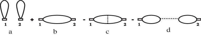
Figure 1: Feynmann diagrams for the averaging of four $\Omega$ fields. The solid lines correspond the Green functions $G^{\Omega}$ of the $\Omega$ field, the dotted lines correspond to the Green functions of the $\lambda$ field. The small boxes are vertices which joint two $\Omega$ fields in some manner. In this sense the diagram $a$ describes the Gaussian contribution, the diagram $b$ describes a correlation, the diagrams $c$ and $d$ describe corrections due to the interaction with the $\lambda$ field. The diagram $c$ is a small correction to the diagram $b$, but the diagram $d$ is of the same order of magnitude as the diagram $b$. For the case of averaging $<\mbox{\boldmath{$\Omega$}}^{2}_{1}\mbox{\boldmath{$\Omega$}}^{2}_{2}>=1$ the diagram $d$ simply cancels the diagram $b$. Notice, that the diagrams $b$ and $d$ are of the order $1/N$ with respect to the diagram $a$.

To avoid this complication we have presented the result in $1/N$ approximation where this complication is not essential.

The effective kinetic Lagrangian and the Hamiltonian in the first $1/2s$ approximation are

$$\Delta{\cal L}_{kin}=s[a_{0}(1-\mbox{\boldmath{$\Omega$}}\cdot\underline{\mbox{\boldmath{$\Omega$}}})+b_{0}({\bf M}^{2}-{\bf M}\cdot\underline{\bf M})-ie_{0}(\mbox{\boldmath{$\Omega$}}\cdot\underline{\bf M}-\underline{\mbox{\boldmath{$\Omega$}}}\cdot{\bf M})],$$ (85)

$${\cal H}=Js^{2}\sum_{l^{\prime}\in<l>}[a_{1}(1-\mbox{\boldmath{$\Omega$}}\cdot\underline{\mbox{\boldmath{$\Omega$}}})+a_{2}(1-\mbox{\boldmath{$\Omega$}}\cdot\mbox{\boldmath{$\Omega$}}^{\prime})+a_{3}(1-\mbox{\boldmath{$\Omega$}}^{\prime}\cdot\underline{\mbox{\boldmath{$\Omega$}}})+b_{1}{\bf M}^{2}+$$

$$+b_{2}{\bf M}\cdot\underline{\bf M}+b_{3}{\bf M}\cdot{\bf M}^{\prime}+b_{4}{\bf M}^{\prime}\cdot\underline{\bf M}-ie_{1}(\mbox{\boldmath{$\Omega$}}\cdot\underline{\bf M}-\underline{\mbox{\boldmath{$\Omega$}}}\cdot{\bf M})-ie_{2}(\mbox{\boldmath{$\Omega$}}^{\prime}\cdot\underline{\bf M}-\underline{\mbox{\boldmath{$\Omega$}}}\cdot{\bf M}^{\prime})],$$

where the notation is the same as in (67), and the constants $a_{0},...,e_{2}$ are

$$a_{i}=a_{i}^{0}+g\alpha_{i},\ \ \ b_{i}=b_{i}^{0}+g\beta_{i},\ \ \ e_{i}=e_{i}^{0}+g\gamma_{i},$$ (86)

$$a_{0}^{0}=1,\ \ b_{0}^{0}=1,\ \ e_{0}^{0}=1,\ \ a_{1}^{0}=-1,\ \ a_{2}^{0}=1,\ \ a_{3}^{0}=0,\ \$$

$$b_{1}^{0}=0,\ \ b_{2}^{0}=1,\ \ b_{3}^{0}=1,\ \ b_{4}^{0}=0,\ \ e_{1}^{0}=-1,\ \ e_{2}^{0}=0,\ \$$

$$\alpha_{0}=2,\ \ \ \beta_{0}=(3-c_{0}+c_{1})/2,\ \ \ \gamma_{0}=(7-c_{0}+c_{1})/4,$$

$$\alpha_{1}=2(1+c_{1}-c_{2}),\ \ \ \alpha_{2}=3+8/\pi^{2}-3c_{0}+2c_{1}+c_{2},$$

$$\alpha_{3}=-4/\pi^{2}+2c_{0}-2c_{1}-c_{2},\ \ \ \beta_{1}=(5-12/\pi^{2}+c_{1}-c_{2})/2,$$

$$\beta_{2}=(-4+8/\pi^{2}+c_{0}-5c_{1}+4c_{2})/2,\ \ \ \beta_{3}=(2-24/\pi^{2}-3c_{0}+c_{1}+2c_{2})/2,$$

$$\beta_{4}=3/\pi^{2},\ \ \ \gamma_{1}=(-6+16/\pi^{2}+9c_{0}-c_{1}-8c_{2})/4,\ \ \ \gamma_{2}=1,$$

where $g=(N-1)/4s$, $i:=0,1,2,3$. The reason why the number of the components $N$ enters in the effective coupling constant as $N-1$ is as follows. The short range fluctuations are directed perpendicular to the long wave fluctuations and their number of independent components is $N-1$.

Now one can write out the effective quadratic form for the Lagrangian (85) in the $\omega,{\bf k}$ representation. Its matrix elements according to the notation (72) are

$$\Lambda^{\Omega}(q)=(1-c_{\omega})[a_{0}+\Delta{\cal J}(a_{1}+a_{3}\gamma_{\bf k})]+\Delta{\cal J}a_{23}(1-\gamma_{\bf k})+\Delta\mu^{2}/2{\cal J},$$ (87)

$$\Lambda^{M}(q)=(1-c_{\omega})[b_{0}-\Delta{\cal J}(b_{2}+b_{4}\gamma_{\bf k})]+\Delta{\cal J}(b_{12}+b_{34}\gamma_{\bf k}),$$

$$\Lambda^{u}(q)=s_{\omega}[e_{0}+\Delta{\cal J}(e_{1}+e_{2}\gamma_{\bf k})],\ \ \ \Lambda^{d}(q)=-\Lambda^{u}(q),$$

where $a_{ij}=a_{i}+a_{j}$ and so on. The Green function is obviously represented by Eq. (75) with $\bar{L}(q)$ in a form

$$\bar{L}(q)=(e_{0}^{2}+\Delta{\cal J}x_{1})[2(1-c_{\omega})+(1-c_{\omega})^{2}\Delta{\cal J}x_{2}+\Delta^{2}\omega^{2}_{\bf k}],$$ (88)

$$\omega^{2}_{\bf k}={\cal J}^{2}[e_{0}^{-2}a_{23}(1-\gamma_{\bf k})+\mu^{2}/({\cal J}^{2}b_{1234})](b_{12}+b_{34}\gamma_{\bf k})$$

where $b_{1234}=b_{12}+b_{34}$, and the explicit form of the coefficients $x_{1},\ x_{2}$ follows from (87). From (11,75,87,88) one can find the spin correlation function in this order in $1/2s$. For that it is necessary to take into account nonlinear corrections to the Eq. (54) which follows from (11) and also corrections to the Green functions in the framework of this formula.

We shall give the explicit result for the correlation radius in this order in $1/2s$ on the basis of Eq. (43). The contribution of different frequencies $\omega$ and momenta ${\bf k}$ in this constraint relation can be separated into two parts. The first part is the high frequency and momentum part. To calculation this contribution it is sufficient to take the Green function $G^{\Omega}(q)$ in the bare approximation (75) because this contribution is of the order $1/2s$. The second contribution which is proportional to the distribution function $n_{\bf k}$ can be considered in the continuum approximation but with $1/2s$ corrections taken into account:

$$G^{\Omega}(q)\simeq\frac{1}{2a^{2}\Delta}\frac{\chi_{\perp}^{-1}}{\omega^{2}+\omega^{2}_{\bf k}},\ \ \ \chi_{\perp}=\tilde{\rho}_{s}/c_{s}^{2},\ \ \ \omega^{2}_{\bf k}=c^{2}_{s}{\bf k}^{2}+\mu^{2},$$ (89)

where $\tilde{\rho}_{s}=Js^{2}a_{23}$, and $c^{2}_{s}=e^{-2}_{0}a_{23}b_{1234}{\cal J}^{2}a^{2}/z$. Now, instead of the Eq. (44) we have

$$(N/4s\tilde{\rho}_{s})\sum_{\bf k}\frac{n_{\bf k}}{\omega_{\bf k}}=R,\ \ \ R=1-g(1+c_{0}+c_{1}),$$ (90)

The factor $R$ inclyudes in itself the direct short wave renormalizations. Performing the integration in the same manner as in (45) we have

$$\mu=T\exp\left(-\frac{2\pi\rho_{s}}{TN}\right),\ \ \ \rho_{s}=\tilde{\rho}_{s}R,\ \ \ \xi=\hbar c_{s}/\mu.$$ (91)

The actual temperature dependence is changed in the pre exponent factor ($T\rightarrow{\cal J}$) if we take into account the long wave fluctuations in the next order in $1/N$ approximation [4].

4 Separation of scales: description of long–wave fluctuations

In some situations one can separate the long wave and short wave spin fluctuations. Our consideration of this problem has a qualitative character and we only sketch the possible approach to it.

The fluctuations of the $M$ field are short wave and the Green functions $G^{M}(q),\ G^{u,d}(q)$ are regular in the long wave limit. Therefore the separation of scales is actual for the $\Omega$ field or the Green function $G^{\Omega}(q)$. This dressed the Green function $G^{\Omega}(q)$ determines the action of the long–wave sigma model. This action is universal and can easily be obtained from the SR Lagrangian (60) or from the Green function (75) by the naive long–wave limit [5]:

$$A=\int{\cal L}_{cont}d\tau d^{2}r,\ \ \ {\cal L}_{cont}=\frac{\chi_{\perp}}{2}\left(\dot{{\bf n}}^{2}+c_{s}^{2}(\partial_{i}{\bf n}\partial_{i}{\bf n})+\mu^{2}{\bf n}^{2}\right)+i\lambda\left({\bf n}^{2}-1\right),$$ (92)

where $\partial_{i}$ is the space derivative for $i:=x,y$; $c_{s}$ is the velocity of sound: $c_{s}^{2}=2J^{2}S^{2}za^{2}$; $\chi_{\perp}=1/2Jza^{2}$ is the transverse susceptibility; $\mu^{2}$ is the mass of the $n$–field in a disordered phase[7]. Because the characteristic low–energy scale $\max(T,\mu)$ is much less than the exchange constant $J,$ the long–wave AF fluctuations contain many universal properties [4]. The connection of the constants which determine these universal properties with parameters of the original Heisenberg model was obtained not by a direct manner but by some calculations in the ordered phase [9, 6].

Our basic idea is to separate scales in the Lagrangian ${\cal L}_{tot}$ (62). The simplest idea is to separate all perturbation theory integrals over ${\bf k}$ into two parts by some separation scale $\Lambda$. But this method introduces some arbitrariness. We will use the scale separation based on some sort of Pauli-Villars transformation. The following identity holds:

$$I=\left(\det(\hat{G})\right)^{-1/2}\int_{-\infty}^{\infty}\frac{d\varphi}{(2\pi)^{1/2}}\exp\left(-\frac{1}{2}\varphi\hat{G}^{-1}\varphi-V(\varphi)\right)=$$ (93)

$$\left(\det(\hat{G}_{1}\hat{G}_{2})\right)^{-1/2}\int_{-\infty}^{\infty}\frac{d\varphi_{1}d\varphi_{2}}{2\pi}\exp\left(-\frac{1}{2}\varphi_{1}\hat{G}_{1}^{-1}\varphi_{1}-\frac{1}{2}\varphi_{2}\hat{G}_{2}^{-1}\varphi_{2}-V(\varphi_{1}+\varphi_{2})\right),$$

where $\hat{G}=\hat{G}_{1}+\hat{G}_{2}$, and $V(\varphi)$ is an arbitrary function such that the integrals in (93) exist. This identity can be easily proved if we introduce for the second integral new variables $\varphi=\varphi_{1}+\varphi_{2}$ and $\psi=\varphi_{1}-\varphi_{2}$. The integration over $\psi$ is Gaussian and can be easily performed. As a result we have the first integral. The identity (93) may be interpreted as follows. Let us choose $\hat{G}=p^{-2}$ and $\hat{G}_{1}=(p^{2}(1+p^{2}/\Lambda^{2}))^{-1},\ \hat{G}_{2}=(p^{2}+\Lambda^{2})^{-1}$. We have achieved the splitting of the Green function of a scalar field $\varphi$ into two parts with the help of the Pauli-Villars transformation. In fact this is a strict integral identity.

Let us apply this method to the Lagrangian ${\cal L}_{tot}$ (62). We represent the field $\Omega$ as a sum two new fields ${\bf n}$ and ${\bf v}$: $\mbox{\boldmath{$\Omega$}}={\bf n}+{\bf v}$. The operators $\hat{G}\equiv\hat{G}^{\Omega}(q)$, $\hat{G}_{1}\equiv\hat{G}^{n}(q)$, and $\hat{G}_{2}\equiv\hat{G}^{v}(q)$, in this case in the $(\omega,k)$ representation may be chosen in the form (72,75):

$$(G^{\Omega}(q))^{-1}=2s\bar{L}(q)/\Lambda^{M}(q)\equiv F(q)\tilde{L}(q),$$ (94)

$$\tilde{L}(q)=2(1-c_{\omega})+\Delta^{2}\omega^{2}_{0{\bf k}},\ \ \ F(q)=2s/(1-c_{\omega}+\Delta{\cal J}(1+\gamma_{\bf k})),$$

$$(G^{n}(q))^{-1}=F(q)\tilde{L}(q)(1+\tilde{L}(q)/\Lambda^{2}),\ \ \ (G^{v}(q))^{-1}=F(q)(\tilde{L}(q)+\Lambda^{2})$$

where the primary dispersion law $\omega_{0{\bf k}}$ is defined in (31). We omit in (94) some small terms of the order $\Delta$ which can be essential only at calculation of the primary free energy (3.2). We assume that $\max(T,\mu)\ll\Lambda\ll{\cal J}$. Only in this case the cut-off momentum $\Lambda$ has a clear meaning.

The fluctuations of the field ${\bf n}$ are long wave and the low frequency. This is motivated by the rapid fall of the Green function $G^{n}(q)$ with increase of the three dimensional momentum $q=(\omega,c_{s}{\bf k}),\ q^{2}=\omega^{2}+c_{s}^{2}{\bf k}^{2}$. As a result the Lagrangian ${\cal L}_{\Omega\lambda}$ reduces to ${\cal L}_{nv\lambda}$ and has the form:

$${\cal L}_{nv\lambda}=(s/2{\cal J})\left({\bf n}\cdot(\hat{q}^{2}+\mu^{2})(1+\hat{q}^{2}/\Lambda^{2}){\bf n}\right)+$$ (95)

$$(1/2){\bf v}\cdot F(\hat{q})(\tilde{L}(\hat{q})+\Lambda^{2}){\bf v}+i\lambda({\bf n}+{\bf v})^{2},$$

The long wave and the low frequency fluctuations of the field ${\bf v}$ are suppressed due to its big mass $\Lambda$, and the long wave and only low frequency fluctuations of the fields $\Omega$ and $\lambda$ are essential. One can check that the long wave theory for the fields $\Omega$ and $\lambda$ practically does not contain ultraviolet divergencies due to the cut off $\Lambda$. Actually the Green function of the $\lambda$ field is determined by the polarization operator $\Pi_{0}(q)$ (50) and in the continuum limit has a form

$$G^{\lambda}(q)=(\Pi_{0}(q))^{-1}=sq^{2}/4{\cal J},\ \ \ q\geq k_{T}.$$ (96)

Now we the have following large momentum behavior of the elements of the diagram technique $G^{n}(q)\sim q^{-4}$, $G^{\lambda}(q)\sim q^{2}$, and $\Gamma(q)\sim q^{0}$, where $\Gamma(q)$ is the vertex. The only divergent diagram is the diagram for the mass operator in the lowest order but it is naturally subtracted one time [7] and after that it is convergent. An additional order of perturbation theory leads to: (a) two additional Green functions $G^{n}(q)$, (b) additional Green function $G^{\lambda}(q)$ (c) additional vertex $\Gamma(q)$, (d) additional integration over q. As a result we have the renormalization factor $R(q)=(G^{n}(q))^{2}G^{\lambda}(q)\Gamma(q)q^{3}\sim q^{-3}$ and the general convergence is improved. This means that the Pauli - Villars regularization is working. It is necessary to stress that without regularization factor $\Lambda^{2}/(q^{2}+\Lambda^{2})$ in the ${\bf n}$ field Green function we have $R\sim q$. This means that the original long wave and low frequency theory is unrenormalizable, and it is not possible to include all divergences in the finite number of objects of the theory. Of course, the parameter $\Lambda$ is an artificial one and must be canceled when we calculate any observable properties due the compensation of the dependence on $\Lambda$ from long wave and short wave contributions.

Let us demonstrate how it is working in some basic example. Let us consider the most important constraint of the theory which determines its phase state: $<\mbox{\boldmath{$\Omega$}}^{2}>=1$. Substituting $\mbox{\boldmath{$\Omega$}}={\bf n}+{\bf v}$ we have

$$<{\bf n}^{2}>=1-<{\bf v}^{2}>,\ \ \ <{\bf n}^{2}>=N\sum_{q}G^{n}(q)\equiv NT\sum_{\omega=2\pi jT}\sum_{\bf k}G^{n}(q)\ \ \$$ (97)

$$<{\bf v}^{2}>=N\sum_{p}G_{v}(\omega,{\bf k})=N\lim_{\Delta\rightarrow 0}\int_{-\pi/\Delta}^{\pi/\Delta}\frac{d\omega}{2\pi}\sum_{\bf k}G_{v}(q),$$

$$G^{n}(q)=\frac{{\cal J}\Lambda^{2}}{s(q^{2}+\mu^{2})(q^{2}+\Lambda^{2})},\ \ \ G^{v}(\omega,{\bf k})=\frac{\Delta^{-1}(1-c_{\omega})+{\cal J}(1+\gamma_{\bf k})}{2s[2\Delta^{-2}(1-c_{\omega})+\omega^{2}_{0{\bf k}}+\Lambda^{2}]}.$$

Here the summation over $j$ for the Green function $G^{n}(q)$ is performed in the limits $\pm\infty$. The main contributions in the integrals in (97) from the Green function $G^{n}$ are from momentum ${\bf k}\leq\Lambda$, and from the Green function $G^{v}$ are from momentum ${\bf k}\geq\Lambda$. This property is general for all integrals with $G^{n},\ G^{v}$. The left hand side of Eq. (97) can be calculated if we reformulate accurately the summation over the frequencies $\omega=2\pi j$ and the integration over the momentum ${\bf k}$ can be extended to infinity (see [1, 4]). When we calculate the right hand side of Eq. (97) we can put the temperature $T$ equal to zero and replace the summation over $\omega$ by an integration and the integration over $\omega$ can be easily performed. The integration over ${\bf k}$ can be performed treating $\Lambda/{\cal J}\ll 1$ as a small parameter. In the part of the integral depending on $\Lambda$, the integration over ${\bf k}$ can be extended to infinity. The other part is independent of $\Lambda$ and can be calculated in the same manner as the constant $c_{M0}$ in Eq. (35). As a result, the constraint (97) has the form

$$\frac{N}{4\pi Js^{2}}(\Lambda+2T\ln(\mu/T))=1+\frac{N\Lambda}{4\pi Js^{2}}-\frac{N}{4s}(1+c_{0}-c_{1}).\ \ \$$ (98)

We can see that dependence on $\Lambda$ is canceled in both sides of Eq. (97) and for $\mu$ we have the expression (46) if we take into account the main order contribution in $1/2s$.

Eq. (98) demonstrates some general properties of the QAF with separation of scales $\xi\ll a$. The role of the classical and quantum spin fluctuations is essentially different. The separation of the spin fluctuation into quantum and classical ones in perturbation theory is determined by the summation over the frequencies $\omega$. The Sommerfeld - Watson transformation gives us the characteristic contributions proportional to $1+2n({\bf k})$, where $n({\bf k})$ is the Plank distribution function, and determines the separation of fluctuations. The quantum fluctuations are independent on the temperature $T$. From the point of view of the long wave theory the quantum fluctuations are divergent in the ultraviolet region. The main contribution into the quantum fluctuations comes from the region in the momentum space $ka\sim 1$. The contribution of the order $k\sim\Lambda$ are small. Actually the second term in the right hand side of (98) is less than the last one by the small parameter $\hbar c_{s}\Lambda/{\cal J}$. This illustrate the idea that the quantum fluctuations in the long wave region are not essential and can be neglected. In this long wave region only the classical fluctuations with the Plank distribution function are essential. In this way we arrive to the ”renormalized classical region” picture [2, 4] for the classical fluctuations. The classical long wave fluctuations possesses some nice properties.

1) They are convergent in the ultraviolet region due to a natural cut off at $k\sim k_{T}$ due to the Plank functions

2) The parameters which determine these fluctuations are the renormalized $\rho_{s}$, $c_{s}^{2}$, $\chi_{\perp}=\rho_{s}/c_{s}^{2}$ that entered in the action (92)

After this discussion the formula (91) for the mass $\mu$ of the $\Omega$ field became obvious: all the quantum renormalizations are included in the renormalized spin stiffness $\rho_{s}$ and simple loop calculation similar to (89,90) gives this result.

The interaction between the long wave ${\bf n}$ and the $\lambda$ fields continue to be essential which leads to the modification of the simple result (90) [2, 4].

5 Discussion

Our approach to the theory of QAF is based on the explicitly rotationally invariant formulation of the pass integral in terms of the spin coherent states. A nontrivial choice of variables permits to formulate the theory based on the saddle point approximation for the field $\Omega$, ${\bf M}$, and $\lambda$. As a result we can find the spin fluctuations at short and at long distances, and at short and at long times.

We work out the method of construction of the perturbation theory over this saddle point. It is not trivial because demands an accurate limit to zero over the time step $\Delta$. This permits to make the theory in some sense similar to the spin wave theory for the calculation of the short distance and short time fluctuations, and similar to the sigma model when we consider the long distance and long time fluctuations. As a result we calculated the free energy and the first corrections to the Green functions of the theory.

We performed the separate scales with the help of Pauli–Villars transformation. This permits to separate out the quantum and the thermal fluctuations. The quantum fluctuations are short waves and the thermal fluctuations are long waves. The fluctuations of the Lagrange multiplier $\lambda$ contains as the short wave as well as long wave contributions.

We believe that the present approach to the QAF will be fruitful in the theory of the AF fluctuations in HTSC superconductors.

Acknowledgments

We are grateful to A.V. Chubukov, I.V. Kolokolov, and S.Sachdev for stimulating discussions; C. Providencia and V.R. Vieira for the accompany discussions; A.M. Finkelstein, and P. Woelfle for critical remarks. One of the authors (V.B.) is grateful for A.L. Chernyshev, L.V. Popovich, and V.A. Shubin for the discussion and cooperation on an earlier step of this work. This work was supported in part by the Portuguese projects PRAXIS/2/2.1/FIS/451/94, V. B. was supported in part by the Portuguese program PRAXIS XXI /BCC/ 11952 / 97, and in part by the Russian Foundation for Fundamental Researches, Grant No 97-02-18546.

Appendix A Invariant coherent states for the rotational group

A.1 Basic formulae for the partition function in terms of the spin coherent states

The partition function for a spin(3) system can be presented as a functional integral over the spin coherent states [10, 11]

$$Z=\lim_{\Delta\rightarrow 0}\int_{-\infty}^{\infty}\cdots\int_{-\infty}^{\infty}\prod_{j=0}^{N_{\tau}-1}\frac{(2s+1)dz^{\prime}_{j}dz^{\prime\prime}_{j}}{\pi(1+|z_{j}|^{2})^{2}}\exp\left(A(z)\right),$$ (99)

$$A(z)=-\Delta\sum_{j=0}^{N_{\tau}-1}\left[{\cal L}_{kin}(j,z)+{\cal H}(j,z)\right],$$ (100)

$$\Delta{\cal L}_{kin}(j,z)=-2s\ln\left(\frac{1+z^{*}_{j+1}z_{j}}{1+|z_{j}|^{2}}\right),\ \ \ {\cal H}(z)=\frac{<z^{*}_{j+1}|\hat{H}|z_{j}>}{<z^{*}_{j+1}|z_{j}>}.$$ (101)

Here $\Delta$ is the time step in the imaginary time $\tau=\Delta j$, $N_{\tau}$ is the number of the time steps: $\Delta N_{\tau}=\beta$; $z_{j}$ is the complex variable for the time step $j$; the integration is performed over $z^{\prime}=\mbox{Re}(z)$ and $z^{\prime\prime}=\mbox{Im}(z)$. It is supposed that the periodic boundary conditions are satisfied $z_{N_{\tau}}=z_{0}$; $A(z)$ is the action, ${\cal L}(\tau)$ is the Lagrangian, ${\cal H}(z)$ is the Hamiltonian. The vector $|z>$ is the spin coherent state which is determined in terms of the reference state $|ref>=|ss>$

$$|z>=\left(1+|z|^{2}\right)^{-s}\exp(z\hat{S}_{-})|ref>,\ \ \ \hat{S}_{z}|sm>=m|sm>,$$ (102)

The coherent state (102) is determined up to the phase factor $\exp(i\Phi(z))$, where $\Phi(z)$ is an arbitrary function $z$, which has no influence on the partition function $Z$, but the kinetic term ${\cal L}_{kin}(j,z)$ is changed as the time component of the Abelian gauge field by the introduction of this phase factor

$${\cal L}_{kin}(j,z)\Rightarrow{\cal L}_{kin}(j,z)-i\Phi(z_{j})+i\Phi(z_{j+1}).$$ (103)

The complex variable $z$ has the geometric interpretation of stereographic projection of a sphere of the radius $1/2$

$$z=\tan(\theta/2)\exp(i\varphi),\ \ \ |z|^{2}=\frac{1-\cos\theta}{1+\cos\theta},$$ (104)

$$\cos\theta=\frac{1-|z|^{2}}{1+|z|^{2}},\ \ \ \sin\theta=\frac{2|z|}{1+|z|^{2}},\ \ \ \tan(\varphi)=\mbox{Im}(z)/\mbox{Re}(z),$$

where $\theta,\varphi$ are the polar and azimuthal angles which determine the unit vector ${\bf n}=\left(\cos\varphi\sin\theta,\sin\varphi\sin\theta,\cos\theta\right)$ which specifies the position on the sphere of radius $1/2$.

In the continuum limit $z_{j+1}\simeq z_{j}+\Delta\dot{z}_{j}$, where the point denotes the derivative with respect to time $\tau$, and the kinetic part of the Lagrangian is equal to

$${\cal L}_{kin}(j,z)=2s\frac{\dot{z}^{*}z}{1+|z|^{2}}=-s(1-\cos\theta)\dot{\varphi}.$$ (105)

Besides that, in the continuum limit the Hamiltonian (99) is determined by the matrix element of the spin operator $\hat{\bf S}$

$$<z|\hat{\bf S}|z>=s{\bf n}.$$ (106)

¿From expressions (105,106) Eq.(6) for ${\cal L}_{kin}(\tau,l)$ and ${\cal H}(\tau,l)$ easily follows.

A.2 Transformation properties of the spin coherent states

Further we want to clarify the reason why for the problem which possesses obvious rotational symmetry for the Heisenberg Hamiltonian (1) the Lagrangian (6) is not explicitly rotationally invariant. The reason lays in the transformation properties of the state $|z>$ under rotations. For further discussion is more convenient to use the state $|{\bf n}>$ which coincides with the state $|z>$ up to a phase factor [10, 11]

$$|{\bf n}>=\exp(is\varphi)|z>=\exp(-i\varphi\hat{S}_{z})\exp(-i\theta\hat{S}_{y})|ref>,$$ (107)

in Eq.(107) is supposed the complex number $z$ and the unit vector ${\bf n}$ are connected by Eq.(104). One can easily check that the state $|{\bf n}>$ satisfies the equation

$$(\hat{\bf S}\cdot{\bf n})|{\bf n}>=s|{\bf n}>.$$ (108)

Eq.(107) can be considered as solution of Eq.(108). Eq. (108) is explicitly rotational invariant but its solution is not. This circumstance was clarified by Perelomov in his paper in which the coherent states where introduced for an arbitrary Lee grope [12]. The rotational grope has three parameters: Euler angles $\varphi,\theta,\psi$ but point on the sphere is parameterized by two parameters $\varphi,\theta$ only. Due to that there is an invariance up to the phase factor

$$|{\bf n}^{\prime}>=\exp(i\Phi({\bf n},\hat{a})\hat{U}(\hat{a})|{\bf n}>,\ \ \mbox{for}\ \ n_{i}=a_{ij}n_{j}.$$ (109)

Here $\hat{a}$ is the $3\times 3$ orthogonal matrix of the three dimensional rotations; $\Phi({\bf n},\hat{a})$ is the phase function which depends on the vector ${\bf n}$ and the matrix $\hat{a}$; $\hat{U}(\hat{a})$ is the operator (matrix) of the $2s+1$ dimensional representation of the rotation $\hat{a}$. Eq. (109) clarifies the situation with an invariance over the three dimensional rotations. The vector $|{\bf n}>$ is not an invariant object but the projector $|{\bf n}><{\bf n}|$ is an invariant object. Now it is obvious why the total action (100) and the partition function (99) are invariant over rotations. Notice that an invariance of the measure of the integration over $z$ is obvious if we pass to variable ${\bf n}$. But the kinetic part of the Lagrangian ${\cal L}_{kin}(j,{\bf n})$ is not invariant over rotations

$$\Delta{\cal L}_{kin}(j,{\bf n})\Rightarrow\Delta{\cal L}_{kin}(j,{\bf n})-i\Phi({\bf n_{j}},\hat{a})+i\Phi({\bf n_{j+1}},\hat{a}).$$ (110)

The transformation (110) is some kind of the Abelian lattice gauge field transformation. It is similar to Eq.(103) but has different meaning.

¿From this discussion it is obvious that the module of the scalar product of two states $|{\bf n}>$ and $|\underline{\bf n}>$ is an invariant over rotations

$$|<\underline{\bf n}|{\bf n}>|=\left(\frac{1+\underline{\bf n}\cdot{\bf n}}{2}\right)^{s}.$$ (111)

Nontrivial invariant over rotation scalar, vector, tensor is determined by the ratio

$$A_{ij,...}=\frac{<\underline{\bf n}|\hat{A}_{ij,...}|{\bf n}>}{<\underline{\bf n}|{\bf n}>},$$ (112)

where $\hat{A}_{ij,...}$ is some operator acting in the spin Hilbert space with definite transformation properties. When the rotational transformation is performed the additional phase factor from numerator and denominator cancel each other. The invariant vector one can get if we choose instead the operator $\hat{A}_{ij,...}$ the spin operator ${\bf S}$, see Eq. (66).

A.3 Invariant coherent states

It seems that a noninvariance over rotations of the spin coherent states $|{\bf n}>$ is their an integral part. However, it is possible to define formally invariant states if we introduce some additional unit vector ${\bf m},\ {\bf m}^{2}=1$ which is orthogonal to the vector ${\bf n},{\bf n}\cdot{\bf m}=0$. After that it is natural to introduce the third unit vector ${\bf k}=[{\bf n}\times{\bf m}]$. This three unit vectors determine a reference frame. One can determine the reference values of these unit vectors or the initial reference frame: ${\bf m}_{0}=(1,0,0),\ {\bf k}_{0}=(0,1,0),\ {\bf n}_{0}=(0,0,1)$. Instead of the transformation (107) which define the state $|{\bf n}>$ we define the state $|{\bf n};{\bf m}>$ with the help of the general rotation from the reference state

$$|{\bf n};{\bf m}>=\exp(-i\varphi\hat{S}_{z})\exp(-i\theta\hat{S}_{y}).\exp(-i\psi\hat{S}_{z})|ref>$$ (113)

Due to our choice of the reference state $|ref>=|ss>$ the last operator exponent factor in (113) in fact is a numerical factor. One can easily find that $\tan\psi=-k_{z}/m_{z}$. For that it sufficient to find three dimensional matrix which rotates the vectors ${\bf n}_{0},{\bf m}_{0}$ into the vectors ${\bf n},{\bf m}$.

Now one can find the Lagrangian ${\cal L}_{kin}(j,{\bf n})$ which is simply equal to

$$\Delta{\cal L}_{kin}(j,{\bf n})=-\ln\left(<\underline{\bf n};\underline{\bf m}|{\bf n};{\bf m}>\right),$$ (114)

where we use a general notation $\underline{x}=x(j+1),\ x\equiv x(j)$. It is follows from Eq.(111) that

$$<\underline{\bf n};\underline{\bf m}|{\bf n};{\bf m}>=\left(\frac{1+\underline{\bf n}\cdot{\bf n}}{2}\right)^{s}Y(\underline{\bf n},\underline{\bf m},{\bf n},{\bf m}),$$ (115)

$${\cal L}_{kin}={\cal L}_{mod}+{\cal L}_{pha},\ \ \$$

$$\Delta{\cal L}_{mod}=-s\ln\left(\frac{1+\underline{\bf n}\cdot{\bf n}}{2}\right),\ \ \ \Delta{\cal L}_{pha}=-\ln\left(Y(\underline{\bf n},\underline{\bf m},{\bf n},{\bf m})\right),$$

where $|Y(\underline{\bf n},\underline{\bf m},{\bf n},{\bf m})|=1$ is a pure phase factor. The Lagrangian ${\cal L}_{mod}$ is pure real, and the Lagrangian ${\cal L}_{pha}$ is pure imaginary.

An explicit form of $Y$ can be found from its in terms of the Euler angels

$$Y^{2}=\exp(is(\underline{\psi}-\psi))<ref|\exp(i\underline{\theta}\hat{S}_{y})\exp(i(\underline{\varphi}-\varphi)\hat{S}_{z})\exp(-i\theta\hat{S}_{y})|ref>/(H.C.).$$ (116)

The matrix element in (116) can be calculated using Wigner d-functions [10, 13] or with the help of z-representation of the spin coherent states (102), [10, 11]

$$Y=\underline{P}^{*}_{\psi}P_{\psi}\underline{P}^{*}_{\varphi}P_{\varphi}P_{n},\ \ \ P_{\varphi}=\left(\frac{n_{x}-in_{y}}{n_{x}+in_{y}}\right)^{s/2},$$ (117)

$$P_{\psi}=\left(\frac{m_{z}+ik_{z}}{m_{z}-ik_{z}}\right)^{s/2},\ \ \ P_{n}=\left(\frac{1+\underline{\bf n}\cdot{\bf n}+\underline{n}_{z}+n_{z}+i[\underline{\bf n}\times{\bf n}]_{z}}{H.C.}\right)^{s}.$$

The factor $Y$ must be an invariant over rotations but this invariability is not obvious from the form (117). In fact $Y$ must be a function of the scalar products $\underline{\bf n}\cdot{\bf n},\ \underline{\bf n}\cdot{\bf m},\ \underline{\bf m}\cdot{\bf k}$ and so on. To find such kind of function we shall use a following trick. Let us calculate the factor $Y$ in a special reference frame where ${\bf m}=(1,0,0),\ {\bf k}=(0,1,0),\ {\bf n}=(0,0,1)$. In this reference frame $P_{\psi}=P_{\varphi}=P_{n}=1$ and $\underline{n}_{x}=\underline{\bf n}\cdot{\bf m},\ \underline{\bf n}_{y}=\underline{\bf n}\cdot{\bf k},\ \underline{m}_{z}=\underline{\bf m}\cdot{\bf n},\ \underline{k}_{z}=\underline{\bf k}\cdot{\bf n}$. As a result we have the following final expression for the Lagrangian ${\cal L}_{pha}$

$$\Delta{\cal L}_{pha}=-\frac{s}{2}\ln\left(\frac{R\underline{R}^{*}}{R^{*}\underline{R}}\right),\ \ \ R=\underline{\bf n}\cdot{\bf m}+i\underline{\bf n}\cdot{\bf k}.$$ (118)

In (118) and all other places we suppose that a quantity $x$ with double underline corresponds to a quantity $x$ without underline. Another form for the Lagrangian ${\cal L}_{pha}$ one can get if we pass to the reference frame where ${\bf n}=(1,0,0),\ {\bf k}=(0,1,0),\ {\bf m}=(0,0,-1)$

$$\Delta{\cal L}_{pha}=-\frac{s}{2}\ln\left(\left[(\underline{\bf n}\cdot{\bf n}+i\underline{\bf n}\cdot{\bf k})\cdot(\underline{\bf m}\cdot{\bf m}+i\underline{\bf k}\cdot{\bf m})\cdot\right.\right.$$ (119)

$$\left.\left.\cdot(1+\underline{\bf n}\cdot{\bf n}-\underline{\bf n}\cdot{\bf m}-i\underline{\bf n}\cdot{\bf k})^{2}\right]\cdot[H.c.]^{-1}\right).$$

Now one can get an expression for the Lagrangian ${\cal L}_{kin}$ in the continuous limit. The magnitude of ${\cal L}_{mod}$ is small over $\Delta$. Using obvious decomposition $\underline{\bf x}\simeq{\bf x}+\Delta\dot{\bf x}$ for ${\bf x}:={\bf n},{\bf m},{\bf k}$ we get from (119) (or technically more complicated from (118)) the following very simple expression for ${\cal L}_{pha}$

$${\cal L}_{pha}=-is{\bf n}\cdot[{\bf m}\times\dot{\bf m}].$$ (120)

One can check that if we choose for the vector ${\bf m}$

$${\bf m}=\frac{{\bf e}_{z}-n_{z}{\bf n}}{\sqrt{1-n^{2}_{z}}},\ \ \,{\bf m}^{2}=1,\ \ \ {\bf n}\cdot{\bf m}=0$$ (121)

$$\mbox{we get for}\ \ \ {\cal L}_{pha}=is(1-\cos\theta)\dot{\varphi},$$

where ${\bf e}_{z}$ is the unit vector along the axis $z$. This result is well known for ${\cal L}_{pha}$.

A.4 Invariant Lagrangian for quantum antiferromagnet

The invariant Lagrangian ${\cal L}_{mod}({\bf n})$ and the Hamiltonian ${\cal H}({\bf n})$ where presented in the text (63,65) but the form of the Lagrangian ${\cal L}_{pha}({\bf n})$ is more complicated and will be discussed in details below.

The situation with the Lagrangian ${\cal L}_{pha}$ is more complicated because it is not expressed in terms of the vectors ${\bf n}$ only (118) but in terms of the vectors ${\bf m}$ and ${\bf k}$ also. These vectors can be presented in terms of the vectors $\mbox{\boldmath{$\Omega$}},{\bf M}$ in a form

$${\bf n}_{a,b}=\pm c_{m}\mbox{\boldmath{$\Omega$}}+s_{m}{\bf l},\ \ \ {\bf m}_{a,b}=c_{m}{\bf l}\mp s_{m}\mbox{\boldmath{$\Omega$}},\ \ \ {\bf k}_{a,b}=\pm[\mbox{\boldmath{$\Omega$}}\times{\bf l}],\ \ \$$ (122)

$$c_{m}=\frac{1-M^{2}/4}{1+M^{2}/4},\ \ \ s_{m}=\frac{M}{1+M^{2}/4},\ \ \ c_{m}^{2}+s_{m}^{2}=1,$$

$${\bf l}=-M^{-1}[\mbox{\boldmath{$\Omega$}}\times{\bf M}],\ \ \ |{\bf l}|=1,\ \ \ {\bf f}=s_{m}{\bf l},\ \ \ {\bf g}=[\mbox{\boldmath{$\Omega$}}\times{\bf f}].$$

These expressions for ${\bf m}$ and ${\bf k}$ are not analytic over the vector ${\bf M}$: they do not have definite limit independent on a direction of vector ${\bf M}$ when it turns to zero. But auxiliary vectors ${\bf f}$ and ${\bf g}$ have definite limit at ${\bf M}$ turns to zero. Now we shall prove that ${\cal L}_{pha}$ summing up over two sublattices ${\rm a}$ and ${\rm b}$ in fact is analytic over the vector ${\bf M}$. According to (118) we have

$$\Delta{\cal L}_{pha}=-\frac{s}{2}\ln\left(\frac{R_{a}\underline{R}_{a}^{*}R_{b}\underline{R}_{b}^{*}}{R_{a}^{*}\underline{R}_{a}R_{b}^{*}\underline{R}_{b}}\right).$$ (123)

Substituting Eqs. (122) for ${\bf n},\ {\bf m}$ and ${\bf k}$ in the Eq. (118) for $R$ we get

$$R_{a,b}=D_{a,b}+E_{a,b},\ \ \ D_{a,b}=\underline{c}_{m}[\pm c_{m}(\underline{\mbox{\boldmath{$\Omega$}}}\cdot{\bf l})+i(\underline{\mbox{\boldmath{$\Omega$}}}\cdot{\bf k})],$$ (124)

$$E_{a,b}=-\underline{c}_{m}s_{m}(\underline{\mbox{\boldmath{$\Omega$}}}\cdot\mbox{\boldmath{$\Omega$}})\mp s_{m}(\underline{\bf f}\cdot\mbox{\boldmath{$\Omega$}})+c_{m}(\underline{\bf f}\cdot{\bf l})\pm i(\underline{\bf f}\cdot{\bf k})$$

The quantities $D_{a,b}$ and $E_{a,b}$ are not analytic over ${\bf M}$ because they contains nonanalytic vectors ${\bf l}$ and ${\bf k}$ explicitly. However, one can introduce new quantities $T_{a,b}=D^{*}_{a,b}R_{a,b}$. Using identity $D_{a}=-D_{b}^{*}$ one can check that the expression (123) for ${\cal L}_{pha}$ will not change if we substitute $R_{a,b}\Rightarrow T_{a,b}$. This property is valid due to compensation of the D-multipliers from sublattices $a$ and $b$. Now one can check that quantities $T_{a,b}$ are analytic over ${\bf M}$

$$T_{a,b}=A_{a,b}+B_{a,b},\ \ \ A_{a,b}=D^{*}_{a,b}D_{a,b}=\underline{c}_{m}^{2}[1-(\underline{\mbox{\boldmath{$\Omega$}}}\cdot\mbox{\boldmath{$\Omega$}})^{2}-(\underline{\mbox{\boldmath{$\Omega$}}}\cdot{\bf f})^{2}],$$ (125)

$$B_{a,b}=D^{*}_{a,b}E_{a,b}=\underline{c}_{m}\{\pm\underline{c}_{m}c_{m}(\underline{\mbox{\boldmath{$\Omega$}}}\cdot\mbox{\boldmath{$\Omega$}})(\underline{\mbox{\boldmath{$\Omega$}}}\cdot{\bf f})+c_{m}(\mbox{\boldmath{$\Omega$}}\cdot\underline{\bf f})(\underline{\mbox{\boldmath{$\Omega$}}}\cdot{\bf f})+$$

$$\hskip 105.2751pt\pm(\underline{\bf f}\cdot{\bf f})(\underline{\mbox{\boldmath{$\Omega$}}}\cdot{\bf f})\mp(\underline{\mbox{\boldmath{$\Omega$}}}\cdot{\bf f})\pm(\underline{\mbox{\boldmath{$\Omega$}}}\cdot\mbox{\boldmath{$\Omega$}})(\mbox{\boldmath{$\Omega$}}\cdot\underline{\bf f})-$$

$$-i[\underline{c}_{m}(\underline{\mbox{\boldmath{$\Omega$}}}\cdot\mbox{\boldmath{$\Omega$}})(\underline{\mbox{\boldmath{$\Omega$}}}\cdot{\bf g})\pm c_{m}(\mbox{\boldmath{$\Omega$}}\cdot\underline{\bf f})(\underline{\mbox{\boldmath{$\Omega$}}}\cdot{\bf g})+c_{m}(\mbox{\boldmath{$\Omega$}}\cdot\underline{\bf g})]\}.$$

Actually, quantities $A_{a,b}$ and $B_{a,b}$ (125) depend only on vectors $\mbox{\boldmath{$\Omega$}},\ {\bf f},\ {\bf g}$ and quantity $c_{m}$ which all are analytic over ${\bf M}$.

Appendix B Calculation integrals and sum over $\omega$

The calculation of integrals and sums over the frequency $\omega$ when the finiteness of the time step $\Delta$ is taken into consideration demands some clarification. We start discussion from the case of the temperature $T$ equal zero and after that pass to the case of the finite temperature.

For the case of the temperature $T$ equal zero the sum over $\omega$ over some function $f(\omega)$ pass into the integral over $\omega$ over the one dimensional $\omega$ Brillouin band inside which $-\pi/\Delta<\omega<\pi/\Delta$ and we are interesting in the integrals

$$I=\int_{-\pi/\Delta}^{\pi/\Delta}f(\omega)d\omega/2\pi.$$ (126)

In the perturbation theory the functions $f(\omega)$ is the rational function of $c_{\omega}=\cos(\omega\Delta)$, i.e. it is a ration of two polynomials from $c_{\omega}$. Such ratio obviously can be presented in a form

$$f(\omega)=P(c_{\omega})+f^{\prime}(c_{\omega}),\ \ \ f^{\prime}(c_{\omega})=Q(c_{\omega})/R(c_{\omega}),$$ (127)

where $P,Q,R$ are polynomials of $c_{\omega}$, and the power of the polynomial $Q$ is less than the power of the polynomial $R$. The polynomial $P(c_{\omega})$ can be easily integrated over $\omega$. The rational function $f^{\prime}(c_{\omega})$ possesses some important properties. 1) This function can be analytically continued in the complex $\omega$ plane. 2) It have some pole singularities in the stripe $-\pi/\Delta<\Re(\omega)<\pi/\Delta,\ -\infty<\Re(\omega)<\infty$. 3) It turns to zero exponentially in upper $-\pi/\Delta<\Re(\omega)<\pi/\Delta,\ 0<\Im(\omega)<\infty$ or low $-\pi/\Delta<\Re(\omega)<\pi/\Delta,\ -\infty<\Im(\omega)<0$ half stripe. 4) The function $f(\omega)$ is periodic in the $\omega$ plane $f(\omega+2\pi/\Delta)=f(\omega)$.

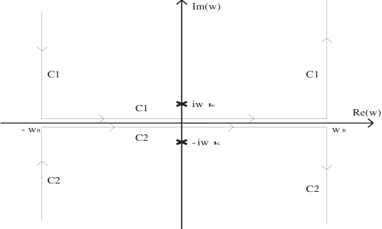
Figure 2: Contours of integration in the complex $\omega$ plane for the calculation of the integral from the function $f^{\prime}(c_{\omega})$. Here on the picture $w\equiv\omega$, $w_{B}=\pi/\Delta$, and $\pm iw_{k}$ are the typical poles of a function $f^{\prime}(c_{\omega})$. The integration is performed over contour $C1$ if the function $f^{\prime}(c_{\omega})$ is decreasing at direction $\Im(\omega)>0$, and the integration is performed over contour $C2$ if the function $f^{\prime}(c_{\omega})$ is decreasing at direction $\Im(\omega)>0$

If all these conditions are valid we can convert the integral (126) from the function $f^{\prime}(c_{\omega})$ into the contour integral in the complex $\omega$ plane. For that one can add to the integral (126) the integral over two vertical half lines which are parallel to the imaginary $\omega$ axis. This two lines are connects points $(-\pi/\Delta,\pm\infty)\rightarrow(-\pi/\Delta,0)$ and $(\pi/\Delta,0)\rightarrow(\pi/\Delta,\pm\infty)$. The choice of the half plane for these two half axes is dictated by the direction in which the function $f(\omega)$ fall down exponentially. Due to periodicity the function $f(\omega)$ the contour integrals over $\omega$ along each pair of this axes compensate each other. If we add these two integrals for the function $f(\omega)$ to the primary integral (126), and also the integral over the segment $(-\pi/\Delta,\pm\infty)\rightarrow(\pi/\Delta,\pm\infty)$ (the last one must be infinitely small) we shall have the closed integral in the $\omega$ plane. It is equal to the sum residues of the function $f(\omega)$ in this half stripe (see Fig. 2).

For the case of the final temperature it is necessary to calculate the following sum

$$I=T\sum_{j=-n_{\tau}}^{n_{\tau}}f(\omega),\ \ \ \omega=2\pi jT,\ \ \ n_{\tau}=(N_{\tau}-1)/2,$$ (128)

where for definiteness the number of the $N_{\tau}$ summation points is odd. Using representation (127) one can easily perform the summation over $\omega$ of the polynomial $P(c_{\omega})$ and for the second term this sum can be converted by the standard manner into the contour integral

$$I^{\prime}=\frac{1}{4\pi i}\int_{C}\cot\left(\frac{\beta\omega}{2}\right)f^{\prime}(c_{\omega})d\omega,$$ (129)

where the contour of the integration is around of the segment of the real $\omega$ axis $-\pi/\Delta<\Re(\omega)<\pi/\Delta$. By the same manner as it was discussed for the case the temperature $T=0$ one can supplement the contour $C$ up to two closed contours over two the half stripes $-\pi/\Delta<\Re(\omega)<\pi/\Delta,\Im\omega>0$ and $-\pi/\Delta<\Re(\omega)<\pi/\Delta,\Im\omega<0$. As a result the sum (128) will be equal to the sum of the residues of the function $0.5\cot(0.5\beta\omega)f^{\prime}(c_{\omega})$ in these two half stripes.

Appendix C Calculation of the free energy

The free energy of simple oscillator is

$$F=\frac{T}{2}\sum_{\omega}\ln\left[\lambda_{\omega}\right],\ \ \ \lambda_{\omega}=2(1-c_{\omega})+\Delta^{2}\omega_{0}^{2},$$ (130)

where $\omega=2\pi jT$, and $-(N_{\tau}-1)/2<j<(N_{\tau}-1)/2$, for definiteness $N_{\tau}$ is odd. It is convenient to represent the eigenvalues $\lambda_{\omega}$ in the form

$$\lambda_{\omega}=\mu_{\omega}\mu^{*}_{\omega},\ \ \ \mu_{\omega}=\alpha+\beta\exp(i\omega\Delta),$$ (131)

$$(\alpha,\beta)\simeq\pm 1+\Delta\omega_{0}/2$$

In terms of the quantities $\mu_{\omega}$ we have for $F$

$$F=T\sum_{\omega}\ln\left[\mu_{\omega}\right]=TN_{\tau}\ln[\alpha]+T\sum_{\omega}\ln[1+(\beta/\alpha)\exp(i\omega\Delta)]$$ (132)

The sum over $\omega$ in Eq. (132) can be easily performed if we expand the logarithmic function in a series over $x=(\alpha/\beta)\exp(i\omega\Delta)$ and take into account only the terms $x^{p}$ with $p=kN_{\tau}$, where $k$ is integer, which give nonzero contributions. The result for $F$ has the form

$$F=TN_{\tau}\ln[\alpha]+T\ln[1+(\beta/\alpha)^{N_{\tau}}].$$ (133)

Using Eq. (131) for $\alpha$, and $\beta$ and conditions $\Delta\omega_{0}\ll 1,\ \Delta N_{\tau}=1/T$ we easily get for the free energy

$$F=\omega_{0}/2+T\ln[1-\exp(-\omega_{0}T)].$$ (134)

It is well known expression for the free energy of the harmonic oscillator.

References

- [1] E. Manousakis, Rev. Mod. Phys. 63, (1991), 1.
- [2] S. Chakravarty, B. I. Halperin, and D. R. Nelson. Phys. Rev. B 39 (1989) 2344.
- [3] A. Sokol, and D. Pines. Phys. Rev. Lett. 71, (1993) 2813.
- [4] A. Chubukov, S. Sachdev, and J. Ye. Phys. Rev. B 49 (1994) 11919.
-
[5]
S.Sachdev, Quantum Antiferromanets in Two Dimensions,
in Low Dimensional Quantum Field Theories for Condensed Matter Physics,
edited by Y. Lu, S.Lundqvist, and G. Morandi, World Scientific, Singapore, 1995. - [6] P. Hasenfratz and F. Niedermayer, Phys. Lett. B 268, 231 (1991); P. Hasenfratz, M. Maggiore and F. Niedermayer, Phys. Lett. B 245, 522 (1990); P. Hasenfratz and F. Niedermayer, Phys. Lett. B 245, 529 (1990).
- [7] A.M. Polyakov, Gauge Fields and Strings, Harwood, New York (1987).
- [8] J. Zinn–Justin, Quantum Field Theory and Critical Phenomena, Oxford Science Publication, Clarendon Press, Oxford (1996).
- [9] J. Igarashi, Phys. Rev., B 46, 10763 (1992).
- [10] J.R. Klauder, and B.S. Skagerstam, Coherent States, World Scientific Publishing, Singapore, 1985.
- [11] V.R. Vieira, P.D. Sacramento, Ann. Phys., 242, 188 (1995); V.R. Vieira, P.D. Sacramento, Nucl. Phys., B448, 331 (1995);
- [12] A.M. Perelomov, Commun. Math. Phys., 26, 222 (1976); A.M. Perelomov, Generalized Coherent States and their Applications, Springer-Verlag, Berlin (1986).
- [13] D.A. Varshalovich, A.N. Moskalev, V.K. Chersonskii, Quantum theory of the angular momentum, Moscow, Nauka, 1975.
- [14] V.I. Belinicher, A.L. Chernyshev, L.V.Popovich, and V.A.Shubin, Czech. Jour. of Phys., 1996, v. 46, Supl.