Validity of the zero-thermodynamic law in off-equilibrium coupled harmonic oscillators

Abstract

In order to describe the thermodynamics of the glassy systems it has been recently introduced an extra parameter, the effective temperature which generalizes the fluctuation-dissipation theorem (FDT) to off-equilibrium systems and supposedly describes thermal fluctuations around the aging state. Using this concept we investigate the applicability of a zeroth thermodynamic law for non-equilibrium systems. In particular we study two coupled systems of harmonic oscillators with Monte Carlo dynamics. We analyze in detail two types of dynamics: 1) sequential dynamics where the coupling between the subsystems comes only from the Hamiltonian and 2) parallel dynamics where there is a further coupling between the subsystems arising from the dynamics. We show that the coupling described in the first case is not enough to make asymptotically the effective temperatures of the two interacting subsystems equalize, the reason being the too small thermal conductivity between them in the aging state. This explains why different interacting degrees of freedom in structural glasses may stay at different effective temperatures without never mutually thermalizing.

I INTRODUCTION

The dynamics of glassy systems has been a subject of intensive research [3]. Despite the fact that glassy systems are off-equilibrium systems, some regularities that allow the rationalization of the problem have been found. One of the most striking regularities is the presence of aging. This means that the correlation and response functions are not only functions of time-differences but also of the time elapsed since the system was prepared [7]. Thus, qualitatively, the longer one waits in the low temperature phase, the smaller the response to an external field will be. A salient feature of systems in equilibrium is the fact that the linear response functions and the equilibrium fluctuations are related by the well known fluctuation-dissipation theorem (FDT) [2]. This relation does not hold for off-equilibrium systems. Several studies of spin-glass mean-field models have shown that a generalization of the fluctuation-dissipation theorem is possible through the definition of the “fluctuation-dissipation ratio” (FDR)[4, 5]:

$$X(t,s)=\frac{TG(t,s)}{\frac{\partial C(t,s)}{\partial s}}(t\geq s),$$ (1)

which is equal to 1 in equilibrium. It turns out that the behavior of the quantity $X(t,s)$ is non trivial in the limit $t,s\to\infty$. If the lowest time $s$ is sent to infinity the quantity $X(t,s)$ becomes a non-trivial function of the autocorrelation $C(t,s)$. This a strong statement which has been proved to hold in the framework of mean-field spin glasses [4, 5]. Moreover, it has been recently recognized that the quantity $X$ is generally related to the Parisi order parameter $P(q)$ which appears in equilibrium studies of spin-glasses providing a natural link between the static and dynamical properties [6].

What is the physical interpretation of $X$? According to relation (1) the fluctuation-dissipation relation would be satisfied if the temperature into the right hand side of (1) were $T/X(t,s)$. This last ratio receives the name of effective temperature and it has been shown [12] that it has some of the good properties of a macroscopic temperature. In fact a proper thermometer coupled to the slow degrees of freedom can measure it. The value of $T_{\rm eff}(t,s)=T/X(t,s)$ would then be different (and higher) than that of the thermal bath. The question about the convenience of this temperature to describe the non-equilibrium behavior has been a subject of controversy in the last years [8]. While there are some evidences (not only theoretical but also experimental [15, 3]) that the violation of FDT gives a good temperature in the thermodynamic sense, it is unclear what properties of standard (i.e. equilibrium) temperatures are common to the non-equilibrium ones.

The motivation of this paper is to answer to the following question: How effective temperatures equalize when two systems out of equilibrium are put in contact? In other words, does there exist a zeroth law for non-equilibrium systems? Let us imagine about a vitrified piece of silica quenched to the room temperature. Because the glass is off-equilibrium its effective temperature is higher than room temperature. But, if we touch the piece of glass it is not hotter than the room temperature. We must conclude that some degrees of freedom within the piece of silica are thermalized to the room temperature while other remain non-thermalized and still hotter. Touching the piece of silica we feel the fast modes, not the slow ones. This poses the question, how is that possible that different interacting degrees of freedom have not reached thermal equilibrium for sufficient long times? Despite of some considerations present in the literature [12, 13] there are no clear answers to this question. We believe that some of them may require a more deep understanding through a detailed analysis of an illustrative example as a previous stage to offer more simple and generic considerations. It is our purpose here to follow this route trying to give a general answer to this question by deriving exact results in the framework of a solvable model.

The model is a set of harmonic oscillators evolving by Monte Carlo dynamics introduced in [9] (hereafter referred as BPR model). The importance of this model relies on the fact that it is exactly solvable and shows one of the main features of glasses, namely aging in correlation and response functions. Our interest will be in considering two coupled sets of harmonic oscillators. Thus, we can see how the main observables are affected by the coupling, in particular how the effective temperature evolves for the two sets of interacting degrees of freedom (represented by the two different sets of harmonic oscillators). The interaction may then appear through the Hamiltonian or through the Monte Carlo dynamics itself. We will discover that the effective temperature for the two sets of oscillators depends on how the coupling is done, and we will understand why in vitreous systems different degrees of freedom may stay at different temperatures without thermalising at very long times. The central idea is that interacting non-equilibrium systems each one with very different effective temperatures may not equalize because the conductivity in the aging state can be extremely small. In this sense the utility of the extension of the zeroth thermodynamic law to the non-equilibrium aging state is questioned due to the smallness of the non-equilibrium conductivities.

The paper is organized as follows. Section II describes the main aspects as well as the interest of the model. Section III describes the two classes of couplings we have considered. Section IV analyzes the case in which the main coupling is ruled by the Monte Carlo dynamics. Section V describes the case where coupling appears only in the Hamiltonian. Sections IV and V show how to solve the dynamics of the system. The reader who is not interested in technical issues can skip them. Section VI discusses the results and the physical consequences of our work. The last section presents the conclusions. Three appendices are devoted to some other technical issues.

II A SIMPLE AND SOLVABLE MODEL OF GLASS

As a simple model of glass we will consider a system of uncoupled harmonic oscillators evolving with Monte Carlo dynamics. The Hamiltonian is:

$$H=\frac{1}{2}K\sum_{i=1}^{N}x_{i}^{2}~{}~{}~{}~{}~{}.$$ (2)

This model was introduced in [9] and was also reviewed in [10, 11].
The low-temperature Monte Carlo dynamics of an ensemble of linear harmonic oscillators shows typical non-equilibrium features of glassy systems like aging in the correlation and response functions. The interest of this model is that the slow dynamics at low temperatures is a consequence of the entropy barriers generated by the low acceptance rate. The simplicity of this model makes it exactly solvable yielding a lot of results about the non-equilibrium behavior.

The Monte Carlo move consists on the following: the $x_{i}$ are moved to $x_{i}+r_{i}/\sqrt{N}$ where $r_{i}$ are random variables Gaussian distributed with zero average and variance $\Delta^{2}.$ The move is accepted according to the transition probability $W(\Delta E)$ which satisfies detailed balance: $W(\Delta E)=W(-\Delta E)\exp(-\beta\Delta E),$ where $\Delta E$ is the change in the Hamiltonian. In Appendix A we show the computation of the correlation and response functions. Here we only quote the main results,

1. Slow decay of the energy. The evolution equation for the energy is Markovian. This simplicity allows for an asymptotic large-time expansion showing that the energy decays logarithmically $E(t)\sim 1/\log(t)$ and the acceptance ratio decays faster $A(t)\sim 1/(t\,\log(t))$.

2. Aging in correlations and responses. The correlation function $C(t,s)$ is defined by:

   $$C(t,s)=\frac{1}{N}\sum_{i=1}^{N}x_{i}(t)x_{i}(s)~{}~{}~{}~{}~{}.$$ (3)

   The response function is calculated by applying an external field to the system. Then, the response function is the variation of the magnetization of the system when the field is applied:

   $$G(t,s)=\left(\frac{\delta M(t)}{\delta h(s)}\right)_{h=0}~{}~{}~{}~{}~{}t>s~{}~{}~{}~{},$$ (4)

   with the magnetization given by,

   $$M(t)=\frac{1}{N}\sum_{i=1}^{N}x_{i}(t)~{}~{}~{}~{}~{}.$$ (5)

   Details on how to solve correlations and responses are given in Appendix A. The final results are equations (108,117). Both correlation and responses show dominant $s/t$ scaling with logarithmic corrections. The asymptotic scaling behavior is given by,

   $$C(t,s)=C(s,s)\frac{L(s)}{L(t)}~{}~{}~{}~{}~{}~{},~{}~{}~{}~{}~{}~{}~{}G(t,s)=G(s,s)\frac{L(s)}{L(t)}\Theta(t-s)~{}~{}~{},$$ (6)

   with $C(s,s)=\frac{2E(s)}{K},G(s,s)=\frac{f(s)}{K}$ where the expression $f(t)$ is given in equation (104) and $L(t)\sim t(\log^{2}(t))$ [16]. The slow decay of the response function shows the presence of long-term memory which manifests as aging in the integrated response function [9].

3. The effective temperature. As said in the introduction, the effective temperature is defined in terms of the FDR eq.(1):

   $$T_{\rm eff}(t,s)=\frac{\frac{\partial C(t,s)}{\partial s}}{G(t,s)}~{}~{}~{}~{}~{}.$$ (7)

   In equilibrium $E(s)=T/2$ and we recover the expected result $T_{\rm eff}=T$. Interestingly (7) yields a result for $T_{\rm eff}$ which only depends on the smallest time $s$. The unique dependence of the effective temperature on the lowest time $s$ is generally believed to be satisfied in the asymptotic large $s$ limit for generic structural glasses and spin-glass models with a one step of replica symmetry breaking. This expectation holds here for all times. At zero temperature when slow motion sets in, the system never reaches the ground state and ages forever. In this regime the effective temperature verifies in the long-time limit (i.e $s\longrightarrow\infty$ ):

   $$T_{\rm eff}(s)=2E(s)+\frac{2}{f(s)}\frac{\partial E(s)}{\partial s}\longrightarrow 2E(s),$$ (8)

   This gives a thermodynamic relationship between the effective temperature and the dynamical energy in the off-equilibrium regime showing how the equipartition theorem can be extended to the glassy regime. The effective temperature measures how a quasi-stationary or adiabatic hypothesis is exact for the present model suggesting that some features of equilibrium thermodynamics may be applied to the aging regime.

III TWO COUPLED SYSTEMS

Now we consider the case in which we couple two systems of harmonic oscillators. In this case it is possible to compute analytically how one system affects the other without loosing the benefit of evaluating Gaussian integrals. The Hamiltonian we have to deal with is:

$$H=\frac{K_{1}}{2}\sum_{i=1}^{N}x_{i}^{2}+\frac{K_{2}}{2}\sum_{i=1}^{N}y_{i}^{2}-\frac{\epsilon}{N}\sum_{i=1}^{N}x_{i}y_{i},$$ (9)

where we take $K_{1}K_{2}>\epsilon^{2}$, otherwise the system has no bounded ground state. We define the following extensive quantities (per oscillator):

$$E_{1}=\frac{K_{1}}{2N}\sum_{i=1}^{N}x_{i}^{2}~{}~{}~{}~{}~{},~{}~{}~{}~{}~{}E_{2}=\frac{K_{2}}{2N}\sum_{i=1}^{N}y_{i}^{2}~{}~{}~{}~{}~{},~{}~{}~{}~{}~{}Q=\frac{1}{N}\sum_{i=1}^{N}x_{i}y_{i}$$ (10)

where $E_{1}$ and $E_{2}$ are the energy of the bare systems while $Q$ is the overlap between them. In this case we also consider Monte-Carlo dynamics, where the transition probability is performed by the Metropolis algorithm which satisfies detailed balance. The random changes in the degrees of freedom $x_{i},y_{i}$ are defined in the same way we have explained in the previous section for the case of a single system. But there are different ways to implement the dynamics in the model depending on the updating procedure of the variables $x_{i},y_{i}$. Here we have analyzed two important and different procedures which yield quite different results:

1. Uncoupled or sequential dynamics. In this case the two sets of variables $x$ and $y$ are sequentially updated. First the $x_{i}$ variables are updated and the move is accepted according to the total change of energy $\Delta E=\Delta E_{1}-\epsilon\Delta Q$. Next, the variables $y_{i}$ are changed and the move accepted according to the energy change $\Delta E=\Delta E_{2}-\epsilon\Delta Q$. This procedure is then iterated. In this case, the dynamics does not affect simultaneously the two sets of variables but each set is updated independently from the other. The only coupling between the two sets of oscillators comes from the explicit coupling term $\epsilon Q$ in the Hamiltonian. Note that for $\epsilon=0$ the dynamics becomes trivial because the dynamical evolutions are that of two independent sets of harmonic oscillators everything reducing to the original model described in section II.

2. Coupled or parallel dynamics. In this first case the $x_{i},y_{i}$ variables are updated in parallel according to the rule $x_{i}\to x_{i}+r_{i}/\sqrt{N}$, $y_{i}\to y_{i}+s_{i}/\sqrt{N}$. The transition probability for that move $W(\Delta E)$ is determined by the change in the total energy $\Delta E=\Delta E_{1}+\Delta E_{2}-\epsilon\Delta Q$ introducing, on top of the explicit coupling term $\epsilon Q$ in the Hamiltonian, an additional coupling between the whole set of oscillators through the parallel updating dynamics. Contrarily to the uncoupled case, the $\epsilon=0$ case is interesting by itself because it shows how this kind of dynamical coupling strongly influences the glassy behavior. In fact, in the limiting case $\epsilon=0$, there will be some changes which make the energy of one of the two systems increase, this change being accepted because the total energy will decrease. Because of that, despite of the fact that there is no direct coupling in the Hamiltonian the dynamics turns out to be strongly coupled.

In what follows we describe the main set of quantities we are interested in. The solution of the dynamical equations for the coupled and uncoupled cases is very similar. The Appendix B shows in detail the derivation of the dynamical solution for the uncoupled case.

A Correlation, overlaps and responses

On top of the time evolution of one-time quantities our interest will also focus on the behavior of two-times quantities such as correlations and responses. These quantities will refer to three classes of systems: the set of oscillators described by the $x$ variables, the set of oscillators described by the $y$ variables and the whole set of $x$ and $y$ variables. In the rest of the paper, as a rule, the subindex 1 will refer to quantities describing the set $x$ of oscillators, the subindex 2 will refer to quantities describing the set $y$ of oscillators and the subindex $T$ will refer to quantities describing the whole set of oscillators $x$ plus $y$. The main set of correlation and response functions we are interested in are:

• Correlations. The correlation function for the sets $x$ and $y$,

  $$C_{1}(t,s)=\frac{1}{N}\sum_{i=1}^{N}x_{i}(t)x_{i}(s)~{}~{}~{}~{}~{},~{}~{}~{}~{}~{}C_{2}(t,s)=\frac{1}{N}\sum_{i=1}^{N}y_{i}(t)y_{i}(s)~{}~{}~{}~{}~{},$$ (11)

  as well as the global correlation $C_{T}(t,s)=\frac{1}{2}(C_{1}(t,s)+C_{2}(t,s))$.

• Overlaps. These are cross-correlations involving different sets of variables:

  $$Q_{1}(t,s)=\frac{1}{N}\sum_{i=1}^{N}y_{i}(t)x_{i}(s)~{}~{}~{}~{}~{},~{}~{}~{}~{}~{}Q_{2}(t,s)=\frac{1}{N}\sum_{i=1}^{N}x_{i}(t)y_{i}(s)~{}~{}~{}~{}~{},$$ (12)

  with $Q_{1}(t,s)=Q_{2}(s,t)$. As we will see later, it is useful to define these two functions $Q_{1},Q_{2}$ which essentially are the same overlap function but acting on different time sectors.

• Response functions. The response function for the sets $x$ and $y$ are defined in the following way. Define the magnetizations for the two sets of oscillators $x$ and $y$,

  $$M_{1}=\frac{1}{N}\sum_{i=1}^{N}x_{i}~{}~{}~{}~{}~{},~{}~{}~{}~{}~{}M_{2}=\frac{1}{N}\sum_{i=1}^{N}y_{i}~{}~{}~{}~{}~{}.$$ (13)

  Consider also two external fields $h_{1}$ and $h_{2}$ conjugated respectively to $M_{1}$ and $M_{2}$,

  $$H=\frac{K_{1}}{2}\sum_{i=1}^{N}x_{i}^{2}+\frac{K_{2}}{2}\sum_{i=1}^{N}y_{i}^{2}-\sum_{i}(h_{1}x_{i}+h_{2}y_{i})-\epsilon\sum_{i}x_{i}y_{i}~{}~{}~{}~{}~{}.$$ (14)

  We define four types of response functions $G_{1,2},G^{\prime}_{1,2}$. The $G_{1}(t,s),G_{2}(t,s)$ functions measure the change in the magnetization $M_{1}(t)$, $M_{2}(t)$ induced by their respective conjugated field $h_{1},h_{2}$ applied at time $s$. These are defined by

  $$G_{i}(t,s)=\left(\frac{\delta M_{i}(t)}{\delta h_{i}(s)}\right)_{h_{i}=0}~{}~{}~{}~{}~{},$$ (15)

  where the index $i=1,2$ represents each one of the systems. Apart from these two response functions we may define the global response function $G_{T}(t,s)$ as the change in the global magnetization $M_{T}=\frac{1}{2}(M_{1}+M_{2})$ induced by a field conjugate to the total magnetization,

  $$G_{T}(t,s)=\left(\frac{\delta M_{T}(t)}{\delta h(s)}\right)_{h=0}=\frac{1}{2}\Bigl{(}G_{1}(t,s)+G_{2}(t,s)\Bigr{)}$$ (16)

  The primed response functions $G_{1}^{\prime}(t,s),G_{2}^{\prime}(t,s)$ functions measure the change in the magnetization in each set of oscillators $M_{1}(t)$, $M_{2}(t)$ induced by a conjugated field (respectively $h_{2},h_{1}$) applied on the other set of oscillators at a time $s$:

  $$G_{i}^{\prime}(t,s)=\left(\frac{\delta M_{i}(t)}{\delta h_{j}(s)}\right)_{h_{j}=0}$$ (17)

  where the indices $i,j=1,2$ are different $i\neq j$. In the absence of a coupling term $\epsilon Q$ in the Hamiltonian (9) the two response functions $G^{\prime}_{1,2}$ vanish but for $\epsilon\neq 0$ they enter into the solution of the dynamical equations.

• Effective temperatures. From the correlation and response functions we may define three effective temperatures: $T_{\rm eff}^{1}$ for the system 1, $T_{\rm eff}^{2}$ for system 2 and $T_{\rm eff}^{T}$ for the global system. These are defined as follows,

  $$T_{\rm eff}^{1}=\left(\frac{\frac{\partial C_{1}(t,s)}{\partial s}}{G_{1}(t,s)}\right)~{}~{}~{}~{}~{},~{}~{}~{}~{}~{}T_{\rm eff}^{2}=\left(\frac{\frac{\partial C_{2}(t,s)}{\partial s}}{G_{2}(t,s)}\right)~{}~{}~{}~{}~{},~{}~{}~{}~{}~{}T_{\rm eff}^{T}=\left(\frac{\frac{\partial C_{T}(t,s)}{\partial s}}{G_{T}(t,s)}\right)~{}~{}~{}~{}~{}.$$ (18)

  We will analyze in detail the three effective temperatures for the coupled and the uncoupled cases. From them we will learn whether the systems equalize their temperatures and how they do.

B Equilibrium regime

Here we present the results for the statics for the general model (9). The equilibrium solution is the stationary state of the dynamics coinciding for both coupled and uncoupled dynamics. The results for the one-time quantities can be simply evaluated from the partition function,

$${\cal Z}=\int_{-\infty}^{\infty}dx\,dy\,\exp(-\beta H),$$ (19)

which involves simple Gaussian integration. By performing the appropriate partial derivatives we calculate the different thermodynamic quantities:

$$E_{1}^{\rm eq}=E_{2}^{\rm eq}=\frac{K_{1}K_{2}T}{2(K_{1}K_{2}-\epsilon^{2})}~{}~{}~{}~{}~{},~{}~{}~{}~{}~{}Q^{\rm eq}=\frac{\epsilon I}{J}=\frac{2\epsilon E_{1}^{\rm eq}}{K_{1}K_{2}}~{}~{}~{}~{}~{},$$ (20)

where the parameters $I,J$ are defined by,

$$I=\frac{E_{1}}{K_{1}}\Delta_{2}^{2}+\frac{E_{2}}{K_{2}}\Delta_{1}^{2}~{}~{}~{}~{}~{},~{}~{}~{}~{}~{}J=\frac{K_{1}\Delta_{1}^{2}}{2}+\frac{K_{2}\Delta_{2}^{2}}{2}~{}~{}~{}~{}~{},$$ (21)

where the total energy $E=E_{1}+E_{2}-\epsilon Q$ is given by the equipartition relation $E=T$. Note that $K_{1}K_{2}-\epsilon^{2}>0$ in order for $E_{1}^{\rm eq},E_{2}^{\rm eq}$ to be positive.

The equilibrium correlations $C$, overlaps $Q$ and responses $G,G^{\prime}$ only depend on the time differences. While the precise form of these functions depends on the particular type of dynamics, the magnetic susceptibilities do not. These are given by:

$$\chi_{1}=\int_{0}^{\infty}G_{1}(t)dt=\frac{K_{2}}{K_{1}K_{2}-\epsilon^{2}},~{}~{}\chi_{2}=\int_{0}^{\infty}G_{2}(t)dt=\frac{K_{1}}{K_{1}K_{2}-\epsilon^{2}},~{}~{}\chi_{T}=\int_{0}^{\infty}G_{T}(t)dt=\frac{1}{2}(\chi_{1}+\chi_{2}),$$ (22)

and are temperature independent as expected for oscillator systems. Nonetheless, in equilibrium the three effective temperatures (18) coincide with the bath temperature $T$.

IV THE DYNAMICALLY UNCOUPLED (OR SEQUENTIAL) CASE

In this section we solve the dynamics of the thermodynamic relevant quantities for the case in which the two subsystems of oscillators are dynamically uncoupled. As explained in the previous section, in this case we make a sequential dynamics avoiding direct dynamical coupling effects coming from the Monte Carlo dynamics. The derivation of the dynamical equations is explained in the Appendix B. The equations for the energies and overlap (10) are written down in (132,133,139),

$$\frac{\partial E_{1}}{\partial t} = -(2E_{1}-\epsilon Q)f_{R_{1}}(t)+\frac{1}{2}\left(\frac{f_{R_{1}}(t)}{\beta}+\frac{K_{1}\Delta_{1}^{2}}{2}ercf(\alpha_{1})\right)$$ (23)

$$\frac{\partial E_{2}}{\partial t} = -(2E_{2}-\epsilon Q)f_{R_{1}}(t)+\frac{1}{2}\left(\frac{f_{R_{2}}(t)}{\beta}+\frac{K_{2}\Delta_{2}^{2}}{2}ercf(\alpha_{2})\right)$$ (24)

$$\frac{\partial Q}{\partial t} = -\left(Q-\frac{2\epsilon E_{2}}{K_{1}K_{2}}\right)f_{R_{1}}(t)-\left(Q-\frac{2\epsilon E_{1}}{K_{1}K_{2}}\right)f_{R_{2}}(t)$$ (25)

with the following definitions:

$$R_{1} = E_{1}-\epsilon Q+\frac{\epsilon^{2}E_{2}}{K_{1}K_{2}}~{}~{}~{}~{}~{},~{}~{}~{}~{}~{}R_{2}=E_{2}-\epsilon Q+\frac{\epsilon^{2}E_{1}}{K_{1}K_{2}},$$ (26)

$$f_{R_{i}}(t) = \frac{K_{i}\Delta_{i}^{2}}{2}\beta\exp\left(-\beta\frac{K_{i}\Delta_{i}^{2}}{2}(1-2R_{i}(t)\beta)\right)erfc(\alpha_{i}(t)(4R_{i}(t)\beta-1))~{}~{}~{}~{}{\rm with}~{}~{}~{}~{}~{}\alpha_{i}=\sqrt{\frac{K_{i}\Delta_{i}^{2}}{16R_{i}}}~{}~{}~{}~{},$$ (27)

where the error function was defined in (103).

Definitions (27) hold for $i=1,2$, each $i$ representing one of the two systems. Note that the whole dynamics is contained in the function $f_{R_{i}(t)}$ . In what follows we will be especially interested in the zero-temperature case where relaxation time diverges and dynamics is slow and glassy. For $T=0$ the function $f_{R_{i}(t)}$ in (27) becomes

$$f_{R_{i}}=\frac{2\alpha_{i}}{\sqrt{\pi}}\exp(-\alpha_{i}^{2})~{}~{}~{}.$$ (28)

A Asymptotic long-time expansion for the one-time quantities

The asymptotic solution of equations (23,24,25) may be guessed from the behavior of the energy (119) for the uncoupled systems. Trying a solution of the type

$$E_{1}=\frac{a}{\log(t)}~{}~{}~{}~{}~{},~{}~{}~{}~{}~{}E_{2}=\frac{b}{\log(t)}~{}~{}~{}~{}~{},~{}~{}~{}~{}~{}Q=\frac{c}{\log(t)}~{}~{}~{}~{}~{},$$ (29)

we can only solve the asymptotic behavior in the limit $\epsilon\approx 0.$ This is a consequence of the fact that the quantities $R_{1}$ and $R_{2}$ are different in general and we have a system of four equations with three parameters. There is not any general solution for this system, but in the limit $\epsilon\approx 0$ the quantities $R_{1}$ and $R_{2}$ become identical to the corresponding energies to leading order yielding only three equations with three unknown parameters ($a,b,c$). In this limit the value of the coefficients $a,b,c$ may be easily obtained yielding

$$a=\frac{K_{1}^{2}K_{2}\Delta_{1}^{2}}{16(K_{1}K_{2}-\epsilon^{2})}~{}~{}~{}~{}~{},~{}~{}~{}~{}~{}b=\frac{K_{1}K_{2}^{2}\Delta_{2}^{2}}{16(K_{1}K_{2}-\epsilon^{2})}~{}~{}~{}~{}~{},~{}~{}~{}~{}~{}c=\frac{\epsilon J}{8(K_{1}K_{2}-\epsilon^{2})},$$ (30)

where $J$ was defined in eq.(21).At first order in logarithmic corrections $1/\log(t)$ we find in the limit $\epsilon\approx 0:$

$$E_{1}=\frac{K_{1}^{2}K_{2}\Delta_{1}^{2}}{16(K_{1}K_{2}-\epsilon^{2})\log(t)}~{}~{}~{}~{}~{},~{}~{}~{}~{}~{}E_{2}=\frac{K_{1}K_{2}^{2}\Delta_{2}^{2}}{16(K_{1}K_{2}-\epsilon^{2})\log(t)}~{}~{}~{}~{}~{},~{}~{}~{}~{}~{}Q=\frac{\epsilon J}{8(K_{1}K_{2}-\epsilon^{2})\log(t)}~{}~{}~{}~{}.$$ (31)

Note that, in the long time limit both energies $E_{1},E_{2}$ tend to zero logarithmically but their relative difference $\frac{E_{1}-E_{2}}{E_{1}}$ stays finite. In the limit of small coupling constant we can do a more refined expansion yielding:

$$E_{1}=\frac{K_{1}^{2}K_{2}\Delta_{1}^{2}}{16(K_{1}K_{2}-\epsilon^{2})}\frac{1}{\log(t)+\frac{1}{2}\log(\log(t))}~{}~{}+~{}~{}{\mathcal{O}}(\frac{1}{\log^{2}(t)}),$$ (32)

$$E_{2}=\frac{K_{1}K_{2}^{2}\Delta_{2}^{2}}{16(K_{1}K_{2}-\epsilon^{2})}\frac{1}{\log(t)+\frac{1}{2}\log(\log(t))}~{}~{}+~{}~{}{\mathcal{O}}(\frac{1}{\log^{2}(t)}),$$ (33)

$$Q=\frac{\epsilon J}{8(K_{1}K_{2}-\epsilon^{2})}\frac{1}{\log(t)+\frac{1}{2}\log(\log(t))}~{}~{}+~{}~{}{\mathcal{O}}(\frac{1}{\log^{2}(t)}),$$ (34)

where we have put explicitly the terms of order $1/\log^{2}(t)$ as sub-dominant corrections. These terms come from the fact that the true expressions for the energies and the overlap should be, in order to match the coefficients in (23,24,25):

$$E_{1}=\frac{a}{\log(At)}~{}~{}~{}~{}~{},~{}~{}~{}~{}~{}E_{2}=\frac{b}{\log(Bt)}~{}~{}~{}~{}~{},~{}~{}~{}~{}~{}Q=\frac{c}{\log(Ct)},$$ (35)

which gives a correction of order $1/\log^{2}(t)$ in expressions (31).

In Fig.1 we show the evolution for the energies and the overlap for two systems of harmonic oscillators with a small value of $\epsilon.$ We also show the asymptotic behavior (32,33,34). We can see that the two energies remain different even at long times. We will see that this feature is very important for describing the non-equilibrium state of the whole system. We can also see that the asymptotic expansions are in good agreement with the numerical solution of the dynamic equations. Nevertheless, there are systematic deviations at long times being consequence of the limited range of validity ($\epsilon\ll 1$) of the asymptotic solution (32,33,34). If $K_{1}\Delta_{1}^{2}=K_{2}\Delta_{2}^{2}$ the energies of the two oscillators become identical (note that equations (102,103,104) only depend on the constant $K\Delta^{2}$) and asymptotic dynamics also.

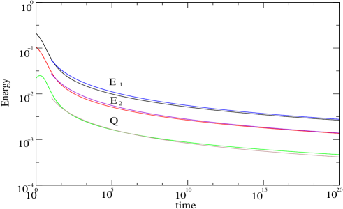
FIG. 1.: The decay of the energies and the overlap for two systems with $K_{1}=2,K_{2}=1,\Delta_{1}=1,\Delta_{2}=1$ and $\epsilon=0.2$. The longest lines are the numerical solution for the dynamic equations, while the shorter ones are the corresponding asymptotic behaviors.

B Correlations and responses.

The set of equations for the four correlation and overlap functions defined in (11,12) can be written as:

$$\frac{\partial}{\partial t}\left(\begin{array}[]{c}C_{1}(t,s)\\ C_{2}(t,s)\\ Q_{1}(t,s)\\ Q_{2}(t,s)\end{array}\right)=-\left(\begin{array}[]{cccc}f_{R_{1}}(t)&0&-\frac{\epsilon}{K_{1}}f_{R_{1}}(t)&0\\ 0&f_{R_{2}}(t)&0&-\frac{\epsilon}{K_{2}}f_{R_{2}}(t)\\ -\frac{\epsilon}{K_{2}}f_{R_{2}}(t)&0&f_{R_{2}}(t)&0\\ 0&-\frac{\epsilon}{K_{1}}f_{R_{1}}(t)&0&f_{R_{1}}(t)\end{array}\right)\left(\begin{array}[]{c}C_{1}(t,s)\\ C_{2}(t,s)\\ Q_{1}(t,s)\\ Q_{2}(t,s)\end{array}\right)$$ (36)

with the subsidiary boundary conditions

$$C_{1}(s,s)=\frac{2E_{1}(s)}{K_{1}}~{}~{}~{}~{}~{},~{}~{}~{}~{}~{}C_{2}(s,s)=\frac{2E_{2}(s)}{K_{2}}~{}~{}~{}~{}~{},~{}~{}~{}~{}~{}Q_{1}(s,s)=Q_{2}(s,s)=Q(s)~{}~{}~{}~{}~{}.$$ (37)

The equilibrium solution can be appropriately worked out because the matrix coefficients are time-independent. If we write the matrix equation in compact form

$$\frac{\partial\vec{C}}{\partial t}=M\vec{C}$$ (38)

with $\vec{C}=(C_{1},C_{2},Q_{1},Q_{2})$ the solution is

$$\vec{C}(t,s)=\vec{C}(s,s)\exp\bigl{(}M_{\rm eq}(t-s)\bigr{)}~{}~{}~{}~{}~{}.$$ (39)

The precise results for correlations and overlaps are reported in the Appendix B (formulae (158-169)), the initial conditions being given in (37). In the non-equilibrium case it is not possible to write down an exact solution for equation (38) for any value of $\epsilon$. The formal solution of (38) is

$$\vec{C}(t,s)={\cal T}\exp\bigl{(}\epsilon\int_{s}^{t}B_{I}(s^{\prime})\bigr{)}\vec{C}(s,s)~{}~{}~{}~{}~{},$$ (40)

which can be worked out perturbatively up to any order around $\epsilon=0$ ($\cal T$ stands for the time ordered product). In the Appendix C, we give some details how to construct such expansion. Up to order $\epsilon^{2}$ the solution for the components $C_{1},C_{2}$ of the four component vector $\vec{C}$ are

$$C_{1}(t,s)=\exp\Bigl{(}-\int_{s}^{t}f_{R_{1}}(x)dx\Bigr{)}\Bigl{(}\frac{2E_{1}(s)}{K_{1}}+\epsilon\frac{Q(s)}{K_{1}}\int_{s}^{t}dt^{\prime}f_{R_{1}}(t^{\prime})e^{\int_{s}^{t^{\prime}}(f_{R_{1}}(x)-f_{R_{2}}(x))dx}+$$ (41)

$$\epsilon^{2}\frac{2E_{1}(s)}{K_{2}K_{1}^{2}}\int_{s}^{t}dt^{\prime}\int_{s}^{t^{\prime}}dt^{\prime\prime}f_{R_{1}}(t^{\prime})f_{R_{2}}(t^{\prime\prime})e^{\int_{t^{\prime\prime}}^{t^{\prime}}(f_{R_{1}}(x)-f_{R_{2}}(x))dx}\Bigr{)},$$ (42)

$$C_{2}(t,s)=\exp\Bigl{(}-\int_{s}^{t}f_{R_{2}}(x)dx\Bigr{)}\Bigl{(}\frac{2E_{2}(s)}{K_{2}}+\epsilon\frac{Q(s)}{K_{2}}\int_{s}^{t}dt^{\prime}f_{R_{2}}(t^{\prime})e^{\int_{s}^{t^{\prime}}(f_{R_{2}}(x)-f_{R_{1}}(x))dx}+$$ (43)

$$\epsilon^{2}\frac{2E_{2}(s)}{K_{1}K_{2}^{2}}\int_{s}^{t}dt^{\prime}\int_{s}^{t^{\prime}}dt^{\prime\prime}f_{R_{2}}(t^{\prime})f_{R_{1}}(t^{\prime\prime})e^{\int_{t^{\prime\prime}}^{t^{\prime}}(f_{R_{2}}(x)-f_{R_{1}}(x))dx}\Bigr{)}.$$ (44)

Similar expansions are obtained from $Q_{1}(t,s),Q_{2}(t,s)$. Here we do not report them because correlations are enough to analyze the effective temperatures. Similarly we can also obtained expressions for the responses as detailed in the Appendix B. The time evolution for the four possible response functions is given by

$$\frac{\partial G_{1}(t,s)}{\partial t} = -\left(G_{1}(t,s)f_{R_{1}}(t)-\frac{f_{R_{1}}(t)}{K_{1}}\delta(t-s)-\frac{\epsilon}{K_{1}}G_{2}^{\prime}(t,s)f_{R_{1}}(t)\right)$$ (45)

$$\frac{\partial G_{2}(t,s)}{\partial t} = -\left(G_{2}(t,s)f_{R_{2}}(t)-\frac{f_{R_{2}}(t)}{K_{2}}\delta(t-s)-\frac{\epsilon}{K_{2}}G_{1}^{\prime}(t,s)f_{R_{2}}(t)\right)$$ (46)

$$\frac{\partial G_{1}^{\prime}(t,s)}{\partial t} = -\left(G_{1}^{\prime}(t,s)f_{R_{1}}(t)-\frac{\epsilon}{K_{1}}G_{2}(t,s)f_{R_{1}}(t)\right)$$ (47)

$$\frac{\partial G_{2}^{\prime}(t,s)}{\partial t} = -\left(G_{2}^{\prime}(t,s)f_{R_{2}}(t)-\frac{\epsilon}{K_{2}}G_{1}(t,s)f_{R_{2}}(t)\right)~{}~{}~{}~{}~{}.$$ (48)

As explained in Appendix B these equations must be solved with the subsidiary boundary conditions,

$$G_{1}(s,s)=\frac{f_{R_{1}}(s)}{K_{1}}~{}~{}~{}~{}~{};~{}~{}~{}~{}~{}G_{2}(s,s)=\frac{f_{R_{2}}(s)}{K_{2}}~{}~{}~{}~{}~{},~{}~{}~{}~{}~{}G_{1}^{\prime}(s,s)=0~{}~{}~{}~{}~{},~{}~{}~{}~{}~{}G_{2}^{\prime}(s,s)=0~{}~{}~{}.$$ (49)

The initial conditions for $G_{1},G_{2}$ come from the delta-terms in their equations. The other two initial conditions for $G_{1}^{\prime},G_{2}^{\prime}$ come from the fact that there is no discontinuous jump in the response function of one system when we apply the field to the other system. This result also holds in the framework of the Langevin dynamics and manifests in the equations for the magnetizations (see in Appendix B (149,151)) as the absence of a field $h_{2}$ in the equation for $M_{1}$ and the absence of a term $h_{1}$ in the equation for $M_{2}$.

In equilibrium the expressions for the responses $G_{1},G_{2}$ are given in the Appendix B. Up to order $\epsilon^{2}$ the expression for the off-equilibrium responses $G_{1},G_{2}$ can be solved analogously as done for the correlations and are given by

$$G_{1}(t,s)=\frac{f_{R_{1}}}{K_{1}}\exp\bigl{(}\int_{s}^{t}f_{R_{1}}(x)dx\bigr{)}\Bigl{(}1+\frac{\epsilon^{2}}{K_{1}K_{2}}\int_{s}^{t}dt^{\prime}\int_{s}^{t^{\prime}}dt^{\prime\prime}f_{R_{1}}(t^{\prime})f_{R_{2}}(t^{\prime\prime})e^{\int_{t^{\prime\prime}}^{t^{\prime}}(f_{R_{1}}(x)-f_{R_{2}}(x))dx}\Bigr{)}$$ (50)

$$G_{2}(t,s)=\frac{f_{R_{2}}}{K_{2}}\exp\bigl{(}\int_{s}^{t}f_{R_{2}}(x)dx\bigr{)}\Bigl{(}1+\frac{\epsilon^{2}}{K_{1}K_{2}}\int_{s}^{t}dt^{\prime}\int_{s}^{t^{\prime}}dt^{\prime\prime}f_{R_{2}}(t^{\prime})f_{R_{1}}(t^{\prime\prime})e^{\int_{t^{\prime\prime}}^{t^{\prime}}(f_{R_{2}}(x)-f_{R_{1}}(x))dx}\Bigr{)}~{}~{}~{}~{}~{}.$$ (51)

V The dynamically coupled (or parallel) case

For the dynamically coupled case the calculations proceed similarly as to the previous dynamically uncoupled case. The evolution equations for the overlap and the energies (10) are:

$$\frac{\partial Q}{\partial t} = -\left(Q-\frac{\epsilon I}{J}\right)f_{E_{N}}(t)$$ (52)

$$\frac{\partial E_{1}}{\partial t} = \frac{K_{1}\Delta_{1}^{2}}{4}erfc\left(\frac{J}{\sqrt{4E_{N}}}\right)+\left(\frac{K_{1}\Delta_{1}^{2}}{2\beta}-2E_{1}\Delta_{1}^{2}K_{1}+\epsilon Q\Delta_{1}^{2}K_{1}\right)\frac{f_{E_{N}}(t)}{2J}$$ (53)

$$\frac{\partial E_{2}}{\partial t} = \frac{K_{2}\Delta_{2}^{2}}{4}erfc\left(\frac{J}{\sqrt{4E_{N}}}\right)+\left(\frac{K_{2}\Delta_{2}^{2}}{2\beta}-2E_{2}\Delta_{2}^{2}K_{2}+\epsilon Q\Delta_{2}^{2}K_{2}\right)\frac{f_{E_{N}}(t)}{2J}~{}~{}~{}~{}~{}.$$ (54)

$I$ and $J$ were defined in (21) and the new quantities $E_{N}$, $f_{E_{N}}$ and $E_{T}$ ($E_{T}$ is not the total energy) are given by

$$E_{N} = E_{T}-2\epsilon QJ+\epsilon^{2}I~{}~{}~{}~{}~{},~{}~{}~{}~{}~{}E_{T}=E_{1}K_{1}\Delta_{1}^{2}+E_{2}K_{2}\Delta_{2}^{2}$$ (55)

$$f_{E_{N}}(t) = J\beta\exp\left(\beta^{2}E_{N}-J\beta\right)erfc\left(\frac{2E_{N}\beta-J}{\sqrt{4E_{N}}}\right)$$ (56)

and the expression (56) at zero-temperature is

$$f_{E_{N}}(t)=\frac{J}{\sqrt{E_{N}\pi}}\exp(-\frac{J^{2}}{4E_{N}})~{}~{}~{}~{}.$$ (57)

A Asymptotic long-time expansion for the one-time quantities

Proceeding similarly as done in the former section we can find the asymptotic expressions for the energies and overlaps. In this case we can find a solution for $\epsilon$ finite due to the fact that in this case we have only one dynamic function $f_{E_{N}}.$ We find, to leading order in $1/\log(t)$

$$E_{1}=\frac{K_{1}K_{2}J}{8(K_{1}K_{2}-\epsilon^{2})\log(t)}~{}~{}~{}~{}~{},~{}~{}~{}~{}~{}E_{2}=\frac{K_{1}K_{2}J}{8(K_{1}K_{2}-\epsilon^{2})\log(t)}~{}~{}~{}~{}~{},~{}~{}~{}~{}~{}Q=\frac{\epsilon J}{4(K_{1}K_{2}-\epsilon^{2})\log(t)}~{}~{}~{}~{}.$$ (58)

Note that, contrarily to results (31) for the dynamically uncoupled case, the energies $E_{1},E_{2}$ asymptotically coincide and the relative difference $(E_{1}-E_{2})/E_{1}$ vanishes in the long-time limit. This difference of behaviors is not casual and has a physical interpretation that we will discuss later. The more precise expansion turns out to be,

$$E_{1}=\frac{K_{1}K_{2}J}{8(K_{1}K_{2}-\epsilon^{2})}\frac{1}{\log(t)+\frac{1}{2}\log(\log(t))}~{}~{}+~{}~{}{\mathcal{O}}(\frac{1}{\log^{2}(t)})$$ (59)

$$E_{2}=\frac{K_{1}K_{2}J}{8(K_{1}K_{2}-\epsilon^{2})}\frac{1}{\log(t)+\frac{1}{2}\log(\log(t))}~{}~{}+~{}~{}{\mathcal{O}}(\frac{1}{\log^{2}(t)})$$ (60)

$$Q=\frac{\epsilon J}{4(K_{1}K_{2}-\epsilon^{2})}\frac{1}{\log(t)+\frac{1}{2}\log(\log(t))}~{}~{}+~{}~{}{\mathcal{O}}(\frac{1}{\log^{2}(t)})~{}~{}~{}~{}~{}.$$ (61)

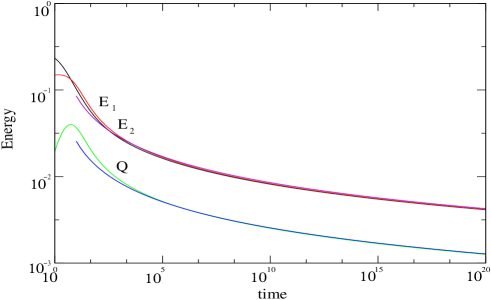
FIG. 2.: The decay of the energies and the overlap for two systems with $K_{1}=2,K_{2}=1,\Delta_{1}=1,\Delta_{2}=1$ and $\epsilon=0.3$. Black lines are the numerical solution for the dynamic equations, while the blue ones are the corresponding asymptotic behaviors.

Let us stress that, contrarily to the dynamically uncoupled or sequential case the previous expressions are valid to any order in $\epsilon$. The origin of the $1/\log^{2}(t)$ terms in previous expressions is the same as in the uncoupled case (32,33,34). In Fig. 2, we show the numerical solution for the evolution of the energies and the overlap as well as the asymptotic expansions (59,60,61).

We have said that the relative difference $(E_{1}-E_{2})/E_{1}$ vanishes in the long-time limit. It is not difficult to see how this happens. The time-evolution for the quantity $E_{1}/E_{2}$ is easy to derive from eqs.(52,53,54) in the asymptotic long-time limit $E_{N}\to 0$. One then finds the following expansion to leading order

$$\frac{E_{1}}{E_{2}}=1-\frac{K_{1}\Delta_{1}^{2}-K_{2}\Delta_{2}^{2}}{2J\log(t)}~{}~{}~{}.$$ (62)

If $K_{1}\Delta_{1}^{2}=K_{2}\Delta_{2}^{2}$ the correction is even smaller.

Interestingly, this leading correction does not depend on $\epsilon$ showing that the two energies $E_{1},E_{2}$ approach each other at a rate determined by the fact that the whole dynamics of the model is coupled and not by the fact that the two oscillator systems are coupled by the presence of a term $\epsilon Q$ in the Hamiltonian. The behavior of this quantity is shown in figure (4) for different values of $\epsilon$ together with the asymptotic expansion (62).

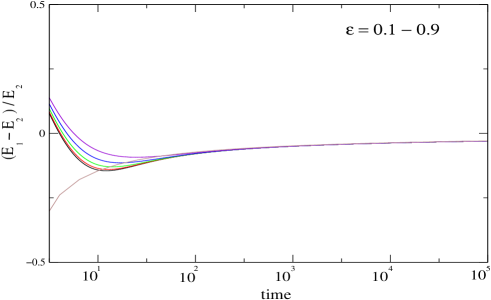
FIG. 3.: Relative energy difference $E_{1}/E_{2}-1$ for two systems with $K_{1}=2,K_{2}=1,\Delta_{1}=1,\Delta_{2}=1$ and $\epsilon=0.1,0.3,0.5,0.7,0.9$ (from top to bottom). The asymptotic prediction (62) is also shown.

B Correlations and responses.

Following similar methods as for the dynamically uncoupled case presented before we can write down the equations for correlations and overlaps

$$\frac{\partial C_{1}(t,s)}{\partial t}=-\left(K_{1}\Delta_{1}^{2}C_{1}(t,s)-\epsilon\Delta_{1}^{2}Q_{1}(t,s)\right)\frac{f_{E_{N}}(t)}{2J}$$ (63)

$$\frac{\partial C_{2}(t,s)}{\partial t}=-\left(K_{2}\Delta_{2}^{2}C_{2}(t,s)-\epsilon\Delta_{2}^{2}Q_{2}(t,s)\right)\frac{f_{E_{N}}(t)}{2J}$$ (64)

$$\frac{\partial Q_{1}(t,s)}{\partial t}=-\left(K_{2}\Delta_{2}^{2}Q_{1}(t,s)-\epsilon\Delta_{2}^{2}C_{1}(t,s)\right)\frac{f_{E_{N}}(t)}{2J}$$ (65)

$$\frac{\partial Q_{2}(t,s)}{\partial t}=-\left(K_{1}\Delta_{1}^{2}Q_{2}(t,s)-\epsilon\Delta_{1}^{2}C_{2}(t,s)\right)\frac{f_{E_{N}}(t)}{2J}~{}~{}~{}~{}~{},$$ (66)

with the subsidiary boundary conditions given by equations (37).

In matrix form these equations reduce to the equation (38). As explained for the uncoupled case, this set of equations can be exactly solved only in the equilibrium regime where the coefficients are time-independent. The solution is then given by the equation (39), the expressions for correlations and overlaps are the formulae (158,165) with $a=-\frac{K_{1}\Delta_{1}^{2}}{2J}f_{E_{N}};b=\frac{\epsilon\Delta_{1}^{2}}{2J}f_{E_{N}};c=\frac{\epsilon\Delta_{2}^{2}}{2J}f_{E_{N}};d=-\frac{K_{2}\Delta_{2}^{2}}{2J}f_{E_{N}}$ and the formulae (160,167) with $a=-\frac{K_{2}\Delta_{2}^{2}}{2J}f_{E_{N}};b=\frac{\epsilon\Delta_{2}^{2}}{2J}f_{E_{N}};c=\frac{\epsilon\Delta_{1}^{2}}{2J}f_{E_{N}};d=-\frac{K_{1}\Delta_{1}^{2}}{2J}f_{E_{N}}$.

In the most general case where the coefficients of the matrix equation are time dependent the exact solution can be written in the closed form (40) which can be expanded to any order in $\epsilon$ as explained in the Appendix C. As in the uncoupled case we present here the results up to order $\epsilon^{2}$ only for the correlations,

$$C_{1}(t,s)=\exp\left(-\frac{K_{1}\Delta_{1}^{2}}{2J}\int_{s}^{t}f_{E_{N}}(x)dx\right)\Bigl{(}\frac{2E_{1}(s)}{K_{1}}+\epsilon\frac{\Delta_{1}^{2}Q(s)}{2J}\int_{s}^{t}dt^{\prime}f_{E_{N}}(t^{\prime})e^{\left(\frac{K_{1}\Delta_{1}^{2}-K_{2}\Delta_{2}^{2}}{2J}\right)\int_{s}^{t^{\prime}}f_{E_{N}}(x)dx}+$$ (67)

$$\epsilon^{2}\frac{2E_{1}(s)\Delta_{1}^{2}\Delta_{2}^{2}}{4J^{2}K_{1}}\int_{s}^{t}dt^{\prime}\int_{s}^{t^{\prime}}dt^{\prime\prime}f_{E_{N}}(t^{\prime})f_{E_{N}}(t^{\prime\prime})e^{\left(\frac{K_{1}\Delta_{1}^{2}-K_{2}\Delta_{2}^{2}}{2J}\right)\int_{t^{\prime\prime}}^{t^{\prime}}f_{E_{N}}(x)dx}\Bigr{)}$$ (68)

$$C_{2}(t,s)=\exp\left(-\frac{K_{2}\Delta_{2}^{2}}{2J}\int_{s}^{t}f_{E_{N}}(x)dx\right)\Bigl{(}\frac{2E_{2}(s)}{K_{2}}+\epsilon\frac{\Delta_{2}^{2}Q(s)}{2J}\int_{s}^{t}dt^{\prime}f_{E_{N}}(t^{\prime})e^{\left(\frac{K_{2}\Delta_{2}^{2}-K_{1}\Delta_{1}^{2}}{2J}\right)\int_{s}^{t^{\prime}}f_{E_{N}}(x)dx}+$$ (69)

$$\epsilon^{2}\frac{2E_{2}(s)\Delta_{2}^{2}\Delta_{1}^{2}}{4J^{2}K_{2}}\int_{s}^{t}dt^{\prime}\int_{s}^{t^{\prime}}dt^{\prime\prime}f_{E_{N}}(t^{\prime})f_{E_{N}}(t^{\prime\prime})e^{\left(\frac{K_{2}\Delta_{2}^{2}-K_{1}\Delta_{1}^{2}}{2J}\right)\int_{t^{\prime\prime}}^{t^{\prime}}f_{E_{N}}(x)dx}\Bigr{)}~{}~{}~{}~{}~{}.$$ (70)

Responses $G_{1,2},G^{\prime}_{1,2}$ can be worked out in a similar way as shown in the Appendix B for the uncoupled case,

$$\frac{\partial G_{1}(t,s)}{\partial t}=-\frac{K_{1}\Delta_{1}^{2}}{2J}\left(G_{1}(t,s)f_{E_{N}}(t)-\frac{f_{E_{N}}(t)}{K_{1}}\delta(t-s)-\frac{\epsilon}{K_{1}}G_{2}^{\prime}(t,s)f_{E_{N}}(t)\right)$$ (71)

$$\frac{\partial G_{2}(t,s)}{\partial t}=-\frac{K_{2}\Delta_{2}^{2}}{2J}\left(G_{2}(t,s)f_{E_{N}}(t)-\frac{f_{E_{N}}(t)}{K_{2}}\delta(t-s)-\frac{\epsilon}{K_{2}}G_{1}^{\prime}(t,s)f_{E_{N}}(t)\right)$$ (72)

$$\frac{\partial G_{1}^{\prime}(t,s)}{\partial t}=-\frac{K_{1}\Delta_{1}^{2}}{2J}\left(G_{1}^{\prime}(t,s)f_{E_{N}}(t)-\frac{\epsilon}{K_{1}}G_{2}(t,s)f_{E_{N}}(t)\right)$$ (73)

$$\frac{\partial G_{2}^{\prime}(t,s)}{\partial t}=-\frac{K_{2}\Delta_{2}^{2}}{2J}\left(G_{2}^{\prime}(t,s)f_{E_{N}}(t)-\frac{\epsilon}{K_{2}}G_{1}(t,s)f_{E_{N}}(t)\right)~{}~{}~{}~{}~{},$$ (74)

with the subsidiary boundary conditions (note that for $G_{1},G_{2}$ they are different from those in (49)),

$$G_{1}(s,s)=\frac{\Delta_{1}^{2}f_{E_{N}}(s)}{2J}~{}~{}~{}~{},~{}~{}~{}~{}G_{2}(s,s)=\frac{\Delta_{2}^{2}f_{2}(s)}{2J}~{}~{}~{}~{},~{}~{}~{}~{}G_{1}^{\prime}(s,s)=0~{}~{}~{}~{},~{}~{}~{}~{}G_{2}^{\prime}(s,s)=0~{}~{}~{}~{}.$$ (75)

It is a simple exercise to check in equilibrium whether these responses give the correct value of the susceptibility (22). In equilibrium responses only depend on the difference of times. As the susceptibility is just the integral of the response function we can integrate the equations (for simplicity we shall consider that $s=0$). Then, the equilibrium susceptibility of every system is just:

$$\chi=\int_{0}^{\infty}G(t)dt~{}~{}~{}~{}~{}.$$ (76)

Integrating the equations for response functions we obtain:

$$G_{1}(\infty)-G_{1}(0) = -\frac{f_{E_{N}}K_{1}\Delta_{1}^{2}}{2J}\left(\chi_{1}+\frac{\epsilon}{K_{1}}\chi_{2}^{\prime}\right)=-\frac{f_{E_{N}}K_{1}\Delta_{1}^{2}}{2JK_{1}}$$ (77)

$$G_{2}^{\prime}(\infty)-G_{2}^{\prime}(0) = -\frac{f_{E_{N}}K_{2}\Delta_{2}^{2}}{2J}\left(\chi_{2}^{\prime}+\frac{\epsilon}{K_{2}}\chi_{1}\right)=0$$ (78)

$$G_{2}(\infty)-G_{2}(0) = -\frac{f_{E_{N}}K_{2}\Delta_{2}^{2}}{2J}\left(\chi_{2}+\frac{\epsilon}{K_{2}}\chi_{1}^{\prime}\right)=-\frac{f_{E_{N}}K_{2}\Delta_{2}^{2}}{2JK_{2}}$$ (79)

$$G_{1}^{\prime}(\infty)-G_{1}^{\prime}(0) = -\frac{f_{E_{N}}K_{1}\Delta_{1}^{2}}{2J}\left(\chi_{1}^{\prime}+\frac{\epsilon}{K_{1}}\chi_{2}\right)=0~{}~{}~{}~{}~{}.$$ (80)

At very long times, ergodicity imposes $G_{1,2}(\infty)=G_{1,2}^{\prime}(\infty)=0$. These equations give the exact results for the equilibrium susceptibilities eqs.(22). In equilibrium the responses can be easily computed and one gets (to keep formulae at minimum we only report the results for $G_{1}$ and $G_{2}$),

$$G_{1}(t,s)=\frac{\Delta_{1}^{2}f_{E_{N}}(s)}{2J}\left(\frac{\lambda_{2}-a}{\lambda_{2}-\lambda_{1}}\exp(\lambda_{1}(t-s))-\frac{\lambda_{1}-a}{\lambda_{2}-\lambda_{1}}\exp(\lambda_{2}(t-s))\right)$$ (81)

$$G_{2}(t,s)=\frac{\Delta_{2}^{2}f_{E_{N}}(s)}{2J}\left(\frac{\lambda_{2}-a}{\lambda_{2}-\lambda_{1}}\exp(\lambda_{1}(t-s))-\frac{\lambda_{1}-a}{\lambda_{2}-\lambda_{1}}\exp(\lambda_{2}(t-s))\right)~{}~{}~{}~{}~{},$$ (82)

with the usual expression (163) for $\lambda_{1},\lambda_{2}$. For $G_{1}$ the values of the constants are:

$$a=-\frac{K_{1}\Delta_{1}^{2}}{2J}f_{E_{N}};~{}~{}~{}~{}~{}b=\frac{\epsilon\Delta_{1}^{2}}{2J}f_{E_{N}};~{}~{}~{}~{}~{}c=\frac{\epsilon\Delta_{2}^{2}}{2J}f_{E_{N}};~{}~{}~{}~{}~{}d=-\frac{K_{2}\Delta_{2}^{2}}{2J}f_{E_{N}}$$ (83)

while for $G_{2}$ the same results (83) are valid but interchanging the indices 1 and 2.

In the general off-equilibrium case the result for $G_{1},G_{2},G^{\prime}_{1},G^{\prime}_{2}$ can be worked out perturbatively. Here we only write the expression up to order $\epsilon^{2}$

$$G_{1}(t,s)=\frac{f_{E_{N}}\Delta_{1}^{2}}{2J}\exp\Bigl{(}-\frac{K_{1}\Delta_{1}^{2}}{2J}\int_{s}^{t}f_{E_{N}}(x)dx\Bigr{)}\times$$ (84)

$$\Bigl{(}1+\epsilon^{2}\frac{\Delta_{1}^{2}\Delta_{2}^{2}}{4J^{2}}\int_{s}^{t}dt^{\prime}\int_{s}^{t^{\prime}}dt^{\prime\prime}f_{E_{N}}(t^{\prime})f_{E_{N}}(t^{\prime\prime})e^{\bigl{(}\frac{K_{1}\Delta_{1}^{2}-K_{2}\Delta_{2}^{2}}{2J}\bigr{)}\int_{t^{\prime\prime}}^{t^{\prime}}f_{E_{N}}(x)dx}\Bigr{)}$$ (85)

$$G_{2}(t,s)=\frac{f_{E_{N}}\Delta_{2}^{2}}{2J}\exp\Bigl{(}-\frac{K_{2}\Delta_{2}^{2}}{2J}\int_{s}^{t}f_{E_{N}}(x)dx\Bigr{)}\times$$ (86)

$$\Bigl{(}1+\epsilon^{2}\frac{\Delta_{2}^{2}\Delta_{1}^{2}}{4J^{2}}\int_{s}^{t}dt^{\prime}\int_{s}^{t^{\prime}}dt^{\prime\prime}f_{E_{N}}(t^{\prime})f_{E_{N}}(t^{\prime\prime})e^{\bigl{(}\frac{K_{2}\Delta_{2}^{2}-K_{1}\Delta_{1}^{2}}{2J}\bigr{)}\int_{t^{\prime\prime}}^{t^{\prime}}f_{E_{N}}(x)dx}\Bigr{)}$$ (87)

VI Results and discussion

First of all we can check that the equilibrium results are the expected ones. It is easy to prove that, independent of the dynamics, the effective temperatures are just the temperature of the bath:

$$T_{\rm eff}^{1}=2E_{1}-\epsilon Q=T,~{}~{}~{}T_{\rm eff}^{2}=2E_{2}-\epsilon Q=T.$$ (88)

Because in equilibrium the energies of the subsystems are the same (see (20)).

A Sequential case

In the off-equilibrium case the results are more interesting. It is easy to verify the following expressions for (18) up to order $\epsilon^{2}$ :

$$T_{\rm eff}^{1}=2E_{1}(s)+\frac{2}{f_{R_{1}}(s)}\frac{\partial E_{1}(s)}{\partial s}-\epsilon Q(s)+\bigl{(}\epsilon Q(s)-\epsilon^{2}\frac{2E_{1}(s)}{K_{1}K_{2}}\bigr{)}\frac{f_{R_{2}}(s)}{f_{R_{1}}(s)}\int_{s}^{t}dt^{\prime}f_{R_{1}}(t^{\prime})e^{\int_{s}^{t^{\prime}}(f_{R_{1}}(x)-f_{R_{2}}(x))dx}$$ (89)

$$T_{\rm eff}^{2}=2E_{2}(s)+\frac{2}{f_{R_{2}}(s)}\frac{\partial E_{2}(s)}{\partial s}-\epsilon Q(s)+\bigl{(}\epsilon Q(s)-\epsilon^{2}\frac{2E_{2}(s)}{K_{1}K_{2}}\bigr{)}\frac{f_{R_{1}}(s)}{f_{R_{2}}(s)}\int_{s}^{t}dt^{\prime}f_{R_{2}}(t^{\prime})e^{\int_{s}^{t^{\prime}}(f_{R_{2}}(x)-f_{R_{1}}(x))dx}~{}~{}~{}~{}~{}.$$ (90)

The expression for the total effective temperature is just

$$T_{\rm eff}^{T}=\frac{\frac{\partial C_{1}(t,s)}{\partial s}+\frac{\partial C_{1}(t,s)}{\partial s}}{G_{1}(t,s)+G_{2}(t,s)}~{}~{}~{}~{}~{},$$ (91)

where the correlations are given by expressions (42,44) and the responses are given by (50,51).

From the equations (89,90) we can see immediately that the effective temperatures are well defined in the regime in which the ratio $\frac{t}{s}$ is finite. Otherwise, the last term in the right hand side of (89) and (90) would diverge. At zero temperature and up to order $\epsilon^{2}$ in the coupling constant, we have found that $E_{1},E_{2},Q$ decrease logarithmically implying that both $f_{R_{1}}$ and $f_{R_{2}}$ decay like $1/t$. Now let us consider $t,s$ both large but $t-s\ll s$. For a weak coupling (i.e $\epsilon\approx 0)$ the value of the effective temperatures are, in the limit $s\rightarrow\infty$ but with $\frac{t}{s}$ finite:

$$T_{\rm eff}^{1}\approx 2E_{1}(s)+{\mathcal{O}}(\epsilon^{2})\approx\frac{K_{1}^{2}K_{2}\Delta_{1}^{2}}{8(K_{1}K_{2}-\epsilon^{2})\log(t)}$$ (92)

$$T_{\rm eff}^{2}\approx 2E_{2}(s)+{\mathcal{O}}(\epsilon^{2})\approx\frac{K_{1}K_{2}^{2}\Delta_{2}^{2}}{8(K_{1}K_{2}-\epsilon^{2})\log(t)}~{}~{}~{}~{}~{}.$$ (93)

This yields in the $s\to\infty$ limit a non vanishing relative difference $T_{\rm eff}^{1}/T_{\rm eff}^{2}-1$. This is a consequence of the fact that the two energies are different in the long-time regime. Note that each effective temperature verifies the equipartition theorem in the limit of long times as expected. The physical interpretation is clear: each system is relaxing towards its equilibrium state slowly and at any time we can consider that the systems are at “quasi-equilibrium” at their corresponding effective temperatures. Obviously the concept of “quasi-equilibrium” is meaningful in a time window smaller than the characteristic time-scale in which the system relaxes (i.e. during this time-scale the effective temperatures do not change), hence we need to impose that $t/s$ is finite.

Let’s think now about the global system. As we have seen, the energies for the two systems remain different even at infinite times. This can be explicitly seen in figure (4) where we show how the relative difference between the energies (or the effective temperatures according to (92,93)) increases monotonically as a function of time (for late times) for any value of $\epsilon$. We may then conclude that a coupling in the Hamiltonian is not enough to reach an equalization of effective temperatures.

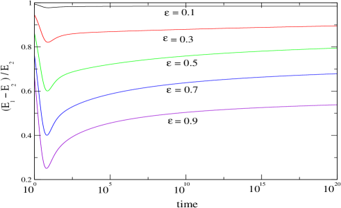
FIG. 4.: Relative energy difference $E_{1}/E_{2}-1$ for two systems with $K_{1}=2,K_{2}=1,\Delta_{1}=1,\Delta_{2}=1$ and different values of $\epsilon=0.1,0.3,0.5,0.7,0.9$. Note that the relative difference increases with time.

This difference of the two effective temperatures implies that there are some degrees of freedom hotter than others. One can then imagine that there is always some kind of heat transfer or current flow going from the “hot degrees” of freedom to the “cold” ones. Then, one may ask why the effective temperatures do not asymptotically equalize. The reason is that the off-equilibrium conductivity may vanish with time fast enough for the heat transfer not to be able to compensate such difference. In this situation, if we now compute the total effective temperature (91) for the whole system we see that in the off-equilibrium regime this temperature does not coincide with the sum of the energies of the systems. This fact fortifies the definition of the effective temperature using the FDR (1) in off-equilibrium systems. For two systems in “local” equilibrium at two different temperatures, despite the fact that each system verifies FDT, the sum of the two systems never verifies FDT unless the two temperatures are equal. In our case, we have two systems which are in “quasi-equilibrium” at two different effective temperatures, so the $T_{\rm eff}^{T}$ would never be the sum of the two energies unless the two effective temperatures $T_{\rm eff}^{1},T_{\rm eff}^{2}$ were the same. In other words, two systems thermodynamically stable at different temperatures are not globally stable when put in contact.

B Parallel dynamics

The effective temperatures (18) can be exactly computed to order $\epsilon^{2}$. In the equilibrium regime, both the full expression derived from (158,165,81,82) and the general approximate solutions (68,70,85,87) up to order $\epsilon^{2}$ computed in the equilibrium regime yield the bath temperature for the three effective temperatures. In the non-equilibrium case, up to order $\epsilon^{2}$, the results are:

$$T_{\rm eff}^{1}=2E_{1}(s)+\frac{4J}{K_{1}\Delta_{1}^{2}f_{E_{N}}(s)}\frac{\partial E_{1}(s)}{\partial s}-\epsilon Q(s)+\bigl{(}\epsilon Q(s)-\epsilon^{2}\frac{2E_{1}(s)}{K_{1}K_{2}}\bigr{)}K_{2}\Delta_{2}^{2}\int_{s}^{t}dt^{\prime}f_{E_{N}}(t^{\prime})e^{\frac{K_{1}\Delta_{1}^{2}-K_{2}\Delta_{2}^{2}}{2}\int_{s}^{t^{\prime}}f_{E_{N}}(x)dx}$$ (94)

$$T_{\rm eff}^{2}=2E_{2}(s)+\frac{4J}{K_{2}\Delta_{2}^{2}f_{E_{N}}(s)}\frac{\partial E_{2}(s)}{\partial s}-\epsilon Q(s)+\bigl{(}\epsilon Q(s)-\epsilon^{2}\frac{2E_{2}(s)}{K_{1}K_{2}}\bigr{)}K_{1}\Delta_{1}^{2}\int_{s}^{t}dt^{\prime}f_{E_{N}}(t^{\prime})e^{\frac{K_{2}\Delta_{2}^{2}-K_{1}\Delta_{1}^{2}}{2}\int_{s}^{t^{\prime}}f_{E_{N}}(x)dx}$$ (95)

The expression for the total effective temperature is just:

$$T_{\rm eff}^{T}=\frac{\frac{\partial C_{1}(t,s)}{\partial s}+\frac{\partial C_{1}(t,s)}{\partial s}}{G_{1}(t,s)+G_{2}(t,s)}$$ (96)

where the correlations are given by expressions (68,70), and the responses are given by (85,87).

As in the case without coupling, the interesting dynamics is when the temperature of the bath is zero. In this case, the energies and the overlap decay to zero logarithmically which implies that $f_{E_{N}}(t)$ vanishes like $1/t$. A careful evaluation of the integrals contributing to the $\epsilon^{2}$ term shown in equations (94,95) reveals that they are a function of $t/s$ which stays finite provided that ratio is finite. As we discussed in the previous uncoupled or sequential case the effective temperatures (94,95) have full sense when we consider times $t/s$ finite so no appreciable transfer of energy between the two systems has still occurred.

It is clear from the asymptotic expressions for the energies and the overlap that in the long-time limit ($s\rightarrow\infty):$

$$\bigl{(}Q(s)-\epsilon\frac{2E_{1}(s)}{K_{1}K_{2}}\bigr{)}\approx\bigl{(}Q(s)-\epsilon\frac{2E_{2}(s)}{K_{1}K_{2}}\bigr{)}\approx\frac{1}{\log^{2}(s)}$$ (97)

While the energies themselves decay as $1/\log(s)$ the relative difference $(Q(s)/E_{1}(s)-\epsilon\frac{2}{K_{1}K_{2}})$ decays like $1/\log(s)$. Up to order $\epsilon^{2}$ we may write, in the limit $s\longrightarrow\infty$ (with $\frac{t}{s}$ finite):

$$T_{\rm eff}^{1}=2E_{1}(s)-\epsilon Q(s)~{}~{}~{}~{}~{},~{}~{}~{}~{}~{}T_{\rm eff}^{2}=2E_{2}(s)-\epsilon Q(s),$$ (98)

because the asymptotic values of the $E_{1}(s)$ and $E_{2}(s)$ are the same the effective temperatures for the subsystems become identical in the long-time limit. Note that the case with dynamic coupling or parallel dynamics is qualitatively different from the case without dynamic coupling or sequential, because now all the degrees of freedom are at the same effective temperature in the long-time limit. Moreover, if we consider the global system it is easy to prove that the total effective temperature defined in (18) is, in the limit $s\rightarrow\infty$ with $\frac{t}{s}$ finite:

$$T_{\rm eff}^{T}=T_{\rm eff}^{1}=T_{\rm eff}^{2}=2E(s)-\epsilon Q(s)$$ (99)

where $E=E_{1}=E_{2}$ and $Q$ are given by (58). This is a consequence of the fact that the energies of the two systems equalize due to the dynamic coupling. Then, the whole system has the same effective temperature and we can define an effective temperature for the global system using FDT. The situation is the same as in equilibrium systems. If we have two systems in equilibrium at a certain temperature $T$, FDT not only holds for each subsystem but also holds for the whole system bringing the temperature of the bath $T$. At higher-orders in $\epsilon$ we expect that all terms with be subleading for $t/s$ to be finite and asymptotically all three temperatures coincide.

If we restrict to the case in which the coupling constant vanishes, $\epsilon=0$, then the systems are still coupled only through the dynamics and we obtain the same qualitatively results:

$$T_{\rm eff}^{T}=T_{\rm eff}^{1}=T_{\rm eff}^{2}=2E(s)$$ (100)

with $E(s)\approx\frac{J}{8\log(s)}$. We conclude that the dynamic coupling does not allow the presence of more than one effective temperature in the whole system because even in the absence of explicit coupling in the Hamiltonian, the dynamics itself makes the energies to equalize in the long-time limit regime.

VII CONCLUSIONS

In this paper we have solved exactly the dynamics of two systems of harmonic oscillators. We focused our attention on the concept of the effective temperature defined through the FDR eq.(1). The effective temperature, a parameter defined by a relation of the correlation and response functions, has been introduced in the context of glass theory in order to understand the physics behind the dynamic behavior of these out-off-equilibrium systems. In this paper we hope to have clarified some aspects behind the physical meaning of this effective temperature.

We have studied two types of couplings between the two subsystems of oscillators, both in an aging state, finding that the way we couple them is crucial for the validity of the zero-temperature law in the off-equilibrium regime to hold. The two cases we studied are the dynamically uncoupled or sequential case and the dynamically coupled or parallel case. In short, for the sequential case the coupling between the variables of the two subsystems in the resulting dynamics arises only through the Hamiltonian term $\epsilon Q$. For the parallel case, the variables of the two subsystems are simultaneously updated leading to further interaction between the two subsystems (on top of the $\epsilon Q$ coupling term in the energy).

We have discovered that for the dynamically uncoupled or sequential case the two subsystems asymptotically reach different effective temperatures which never equalize. So the whole system is divided in two parts, each part characterized by its own effective temperature. The explanation for this odd behavior lies behind the time dependence of the off-equilibrium thermal conductivity which decays very quickly to allow for an asymptotic equalization of the two effective temperatures. This raises the question whether different interacting degrees of freedom do eventually reach the same effective temperature in the asymptotic regime, condition tightly related to the validity of the zeroth law for the off-equilibrium aging state. Our conclusion is that the zeroth law is probably valid but hardly effective due to the very small conductivity between the two subsystems in the aging state. A calculation of the thermal conductivity in this model will be shown elsewhere [17] and reveals that it decreases very quickly with time, the heat transfer being unable to compensate for the difference of the effective temperatures of the two subsystems.

For the dynamically coupled or parallel case, the two effective temperatures equalize and the two subsystems are in a sort of thermal equilibrium between them in the aging state. Consequently, the union of the two subsystems has an effective temperature which coincides with the temperature of each subsystem. In this case, the direct coupling of the two subsystems through the parallel dynamics makes the conductivity much larger than in the sequential case so in this case a zero-th law for the aging state is effective and holds. In fact, these results are also valid when we consider the particular case $\epsilon=0$ in which the dynamics in itself is enough to equalize the effective temperatures.

From these two type of couplings the first one is the only realistic. Dynamics in real structural glasses involves short scale motions of atoms and coupling between the different degrees of freedom occurs at the level of the energy or Hamiltonian and never at the level of the dynamics (at least in the classical regime). The results of this paper explain then why different degrees of freedom in structural glasses can stay at different effective temperatures forever. The off-equilibrium conductivity or heat transfer between the different degrees of freedom is small enough for the equalization of the effective temperatures associated to the different degrees to never occur. This explains why when we touch a piece of glass we feel it at the room temperature. The heat transfer coming from the hotter non-thermalized degrees of freedom is extremely small. Before finishing we must note one particular feature of our model. All the calculations were done at zero temperature where the energy vanishes asymptotically. The fact that the energy (and consequently the conductivity) of the system is exhausted in the asymptotic limit can lead to a pathological behavior not present in structural glasses at finite temperature. Nevertheless, the fact that the thermal conductivity vanishes much faster than the energy itself, suggests that the vanishing of the conductivity is not related to zero-temperature dynamics.

In the present calculation we have focused on the interaction between two subsystems, both in the aging state. When one of the subsystems is in an aging state and the other is in equilibrium the analysis proceeds similarly, the conclusion being that the non-thermalized subsystem determines the rate of heat transfer and hence the measurement of the effective temperature. The value of the effective temperature measured by a thermometer and other related questions can be analyzed in detail in the present model and will be presented elsewhere [17].

To conclude, although a zero-th law for non-equilibrium glassy systems may hold, it is hardly effective because of the small energy transfer occurring between degrees of freedom at different effective temperatures. It would be very interesting to pursue this investigation further by studying other solvable examples and showing that what we have exemplified here is a generally valid for structural glasses as well as for other glassy systems.

Acknowledgements. We are grateful to M. Picco for a careful reading of the manuscript. A. G. is supported by a grant from the University of Barcelona. F. R is supported by the Ministerio de Educación y Ciencia in Spain (PB97-0971).

In this appendix we show how derive the results for the correlation and the response functions in  [9] in order to understand the techniques we will use throughout this paper. In that model, the system is constituted by $N$ uncoupled harmonic oscillators which evolve with Monte Carlo dynamics. The energy of this system is

$$E({x_{i}})=\frac{1}{2}K\sum_{i}x_{i}^{2}~{}~{}~{}~{}~{}.$$ (101)

The result for the dynamical evolution for the energy is:

$$\frac{\partial E}{\partial t}=\frac{a_{c}}{2}\left(\frac{1-4E\beta}{a_{c}\beta}f(t)+erfc(\alpha)\right)~{}~{}~{}~{}~{},$$ (102)

where we have defined the quantities

$$a_{c}=\frac{1}{2}K\Delta^{2}~{}~{}~{}~{}~{},~{}~{}~{}~{}~{}\alpha=\sqrt{\frac{K\Delta^{2}}{16E}},~{}~{}~{}~{}erfc(x)=\frac{2}{\sqrt{\pi}}\int_{x}^{\infty}\exp(-x^{2})dx,$$ (103)

$$f(t)=a_{c}\beta\exp\left(-\beta\frac{K\Delta^{2}}{2}(1-2E(t)\beta)\right)erfc(\alpha(t)(4E(t)\beta-1))~{}~{}~{}~{}~{}.$$ (104)

The stationary solution is just $E=\frac{1}{2}T$ as expected. Another important quantity is the acceptance rate which is the number of accepted Monte Carlo movements at a time $t$:

$$A(t)=\frac{1}{2}\left(\frac{f(t)}{a_{c}\beta}+erfc(\alpha)\right)~{}~{}~{}~{}~{}.$$ (105)

In the same way we can compute the equation for the correlation function defined as:

$$C(t,s)=\frac{1}{N}\sum_{i=1}^{N}x_{i}(t)x_{i}(s)~{}~{}~{}~{}~{},$$ (106)

and the evolution of the correlation function is given by the equation

$$\frac{\partial C(t,s)}{\partial t}=-f(t)C(t,s)~{}~{}~{}~{}~{},$$ (107)

where the quantity $f(t)$ has been previously defined in (104). The solution for the correlation function (which depends explicitly on two times) is:

$$C(t,s)=\frac{2E(s)}{K}\exp\left(-\int_{s}^{t}f(x)dx\right)~{}~{},$$ (108)

where we have to add the initial condition $C(s,s)=\frac{2E(s)}{K}.$ In order to compute the equation for the response function defined by,

$$G(t,s)=\left(\frac{\delta M(t)}{\delta h(s)}\right)_{h=0}~{}~{},$$ (109)

we have to consider the Hamiltonian perturbed by a small external field

$$H=\frac{K}{2}\sum_{i=1}^{N}x_{i}^{2}-h\sum_{i}x_{i}~{}~{}~{}~{}~{}.$$ (110)

Then we compute the dynamical evolution for the magnetization, which in our model is defined by: $M=\frac{1}{N}\sum_{i=1}^{N}x_{i}$ yielding:

$$\frac{\partial M(t)}{\partial t}=-\left(M(t)-\frac{h}{K}\right)f_{E^{\prime}}(t)\Theta(t-s)~{}~{}~{}~{}~{},$$ (111)

where we have defined a ’new’ energy as:

$$E^{\prime}=E-Mh+\frac{h^{2}}{2K}~{}~{}~{}~{}~{}.$$ (112)

The quantity $f_{E^{\prime}}(t)$ is identically defined as in (104) but with the new energy $E^{\prime}$. Note that in the case in which $h=0$ the magnetization will always be zero because of the initial condition we consider, i.e $M(0)=0$. Also, when we compute the evolution for the response function, the first term in the right hand side of the (111) is just the response. Then we have to analyze carefully the second term (which is proportional to the external field) in the right hand side of (111). First of all, we write

$$G(t,s)\approx\frac{\Delta M(t)}{h\Delta s}~{}~{}~{}~{}~{},~{}~{}~{}~{}~{}\frac{\partial G(t,s)}{\partial t}\approx\frac{\frac{\Delta M(t)}{\Delta t}}{h\Delta s}~{}~{}~{}~{}~{}.$$ (113)

We consider the variation of the magnetization as follows

$$\frac{\Delta M}{\Delta t}=\Delta s\frac{\partial}{\partial s}\left(\frac{\partial M(t)}{\partial t}\right)\Theta(t-s)+\Delta s\frac{\partial M(t)}{\partial t}\delta(t-s)~{}~{}~{}~{}~{},$$ (114)

and by keeping only the linear term in $h$ in the second term of the r.h.s in (114) we get

$$\frac{\Delta M}{\Delta t}=\Delta s\frac{h}{K}\frac{\partial f(t)}{\partial s}\Theta(t-s)+\Delta s\frac{h}{K}f(t)\delta(t-s)~{}~{}~{}~{}~{}.$$ (115)

The first term in the r.h.s of (115) is obviously zero and only the the second term gives a non-vanishing contribution. So the evolution for the response function is

$$\frac{\partial G(t,s)}{\partial t}=-f(t)\left(G(t,s)-\frac{1}{K}\delta(t-s)\right)~{}~{}~{}~{}~{},$$ (116)

whose solution is

$$G(t,s)=\frac{f(s)}{K}\exp\left(-\int_{s}^{t}f(x)dx\right)\Theta(t-s)~{}~{}~{}~{}~{}.$$ (117)

Now, we are in position to compute the effective temperature based on the violation of FDT

$$T_{\rm eff}=\left(\frac{\frac{\partial C(t,s)}{\partial s}}{G(t,s)}\right)=2E(s)+\frac{1}{f(s)}\frac{\partial E(s)}{\partial s}~{}~{}~{}~{}~{}.$$ (118)

Note that the effective temperature only depends on the smallest time $s$. This feature is due to the simplicity of the model. In this model, due to the finite amplitude of the Monte Carlo movements the system never reaches the ground state $\{x_{i}=0\}$. In fact, Monte Carlo dynamics induces entropic barriers which manifest as activated behavior for the relaxation time. The interesting dynamics is found when we study the relaxation of the system at zero temperature. To obtain the dynamical equations at zero temperature we have to consider only the negative changes in the energy. It can be seen that in the long time limit the relaxation of the energy is logarithmic

$$E(t)\approx\frac{K\Delta^{2}}{16}\frac{1}{\log\left(\frac{2t}{\sqrt{\pi}}\right)+\frac{1}{2}\log(\log\left(\frac{2t}{\sqrt{\pi}}\right))}~{}~{}~{}~{}~{},$$ (119)

moreover, we obtain the following asymptotic behavior of the function $f(t)$ and the acceptance rate:

$$f(t)\approx\frac{1}{t}\left(1+\frac{\frac{1}{2}\log(\log\left(\frac{2t}{\sqrt{\pi}}\right))}{\log\left(\frac{2t}{\sqrt{\pi}}\right)}\right)^{\frac{1}{2}},~{}~{}~{}A(t)\approx\frac{1}{4t\log\left(\frac{2t}{\sqrt{\pi}}\right)}.$$ (120)

For the long time behavior of the correlation and the response functions we obtain to leading order in $\log(s)/\log(t)$

$$C(t,s)=\frac{2E(s)}{K}C_{norm}(t,s)~{}~{}~{}~{},~{}~{}~{}~{}C_{norm}(t,s)\approx\frac{s\log^{2}\left(\frac{2s}{\sqrt{\pi}}\right)}{t\log^{2}\left(\frac{2t}{\sqrt{\pi}}\right)}~{}~{}~{}~{},~{}~{}~{}~{}G(t,s)\approx\frac{1}{Kt}\left(\frac{\log\left(\frac{2s}{\sqrt{\pi}}\right)}{\log\left(\frac{2t}{\sqrt{\pi}}\right)}\right)^{2}~{}~{}~{}~{}.$$ (121)

APPENDIX B: SOLUTION OF THE DYNAMICALLY UNCOUPLED OR SEQUENTIAL CASE

In this appendix we show explicitly the detailed calculations for the case in which we sequentially update the two subsystems. Note that each subsystem is updated in parallel but no simultaneous updating of the whole system is performed so there is no direct coupling of the two subsystems through the dynamics but only through an explicit coupling term $\epsilon Q$ in the Hamiltonian. We have to take into account this fact when we compute the distribution probability for a change in the energy. The Hamiltonian we have to deal with is

$$H=\frac{K_{1}}{2}\sum_{i=1}^{N}x_{i}^{2}+\frac{K_{2}}{2}\sum_{i=1}^{N}y_{i}^{2}-\epsilon\sum_{i=1}^{N}x_{i}y_{i}~{}~{}~{}~{}.$$ (122)

The main quantities we work with are

$$E_{1}=\frac{K_{1}}{2N}\sum_{i=1}^{N}x_{i}^{2}~{}~{}~{}~{}~{},~{}~{}~{}~{}~{}E_{2}=\frac{K_{2}}{2N}\sum_{i=1}^{N}y_{i}^{2}~{}~{}~{}~{}~{},~{}~{}~{}~{}~{}Q=\frac{1}{N}\sum_{i=1}^{N}x_{i}y_{i}~{}~{}~{}~{}~{},$$ (123)

where $E_{1}$ and $E_{2}$ are the energy of the bare systems while $Q$ is the overlap between them.

The Monte Carlo updating procedure is the following. First all the $x_{i}$ are moved to $x_{i}+r_{i}/\sqrt{N}$ where the $r_{i}$ are random variables Gaussian distributed with zero average and variance $\Delta_{1}^{2}.$ The move is accepted according to a rule defined by an acceptance probability $W(\Delta E)$ which satisfies detailed balance: $W(\Delta E)=W(-\Delta E)\exp(-\beta\Delta E),$ where $\Delta E$ is the change in the Hamiltonian. Later all the $y_{i}$ are moved to $y_{i}+s_{i}/\sqrt{N}$, where the $s_{i}$ are random variables Gaussian distributed with zero average and variance $\Delta_{2}^{2}.$ The same transition probability is now applied for the $y_{i}$ variables. This sequential updating of the $x_{i}$ and $y_{i}$ variables is then iterated. Note that the coupling in the dynamics only appears through the change $\epsilon\Delta Q$ of the total energy.

Now we compute the distribution probability of a change in the energy of the first system. This probability distribution can be expressed

$$P(\delta E_{1})=\int_{-\infty}^{\infty}\delta\left(\delta E_{1}-K_{1}\sum_{i}\left(\frac{r_{i}x_{i}}{\sqrt{N}}+\frac{r_{i}^{2}}{2N}\right)+\epsilon\sum_{i}\frac{r_{i}y_{i}}{\sqrt{N}}\right)\left(\prod_{i}\frac{dr_{i}}{\sqrt{2\pi\Delta_{1}^{2}}}\exp\left(-\frac{r_{i}^{2}}{2\Delta_{1}^{2}}\right)\right)$$ (124)

and in the same way we can compute the probability for the other system:

$$P(\delta E_{2})=\int_{-\infty}^{\infty}\delta\left(\delta E_{2}-K_{2}\sum_{i}\left(\frac{s_{i}y_{i}}{\sqrt{N}}+\frac{s_{i}^{2}}{2N}\right)+\epsilon\sum_{i}\frac{s_{i}x_{i}}{\sqrt{N}}\right)\left(\prod_{i}\frac{ds_{i}}{\sqrt{2\pi\Delta_{2}^{2}}}\exp\left(-\frac{s_{i}^{2}}{2\Delta_{2}^{2}}\right)\right)~{}~{}~{}~{}~{}.$$ (125)

Using the integral representation of the delta function:

$$\delta(m)=\frac{1}{2\pi}\int_{-\infty}^{\infty}\exp\left(i\lambda m\right)d\lambda~{}~{}~{}~{}~{},$$ (126)

we obtain

$$P(\delta E_{1})=\frac{1}{\sqrt{4\pi K_{1}R_{1}\Delta_{1}^{2}}}\exp\left(-\frac{(\delta E_{1}-\frac{K_{1}\Delta_{1}^{2}}{2})^{2}}{4K_{1}R_{1}\Delta_{1}^{2}}\right)~{}~{}~{}~{}~{},$$ (127)

$$P(\delta E_{2})=\frac{1}{\sqrt{4\pi K_{2}R_{2}\Delta_{2}^{2}}}\exp\left(-\frac{(\delta E_{2}-\frac{K_{2}\Delta_{2}^{2}}{2})^{2}}{4K_{2}R_{2}\Delta_{2}^{2}}\right)~{}~{}~{}~{}~{},$$ (128)

with the quantities

$$R_{1}=E_{1}-\epsilon Q+\frac{\epsilon^{2}E_{2}}{K_{1}K_{2}}~{}~{}~{}~{}~{},~{}~{}~{}~{}~{}R_{2}=E_{2}-\epsilon Q+\frac{\epsilon^{2}E_{1}}{K_{1}K_{2}}~{}~{}~{}~{}~{}.$$ (129)

Note that due to the explicit coupling $\epsilon$ the probability of a change in the energy of one system not only depends on their energy, but also on the energy of the other system and the overlap. Now, we can compute the evolution of the energies

$$\frac{\partial E_{1}}{\partial t}=\int_{-\infty}^{0}d(\delta E_{1})\delta E_{1}P(\delta E_{1})+\int_{0}^{\infty}d(\delta E_{1})\delta E_{1}P(\delta E_{1})\exp(-\beta\delta E_{1})~{}~{}~{}~{}~{},$$ (130)

$$\frac{\partial E_{2}}{\partial t}=\int_{-\infty}^{0}d(\delta E_{2})\delta E_{2}P(\delta E_{2})+\int_{0}^{\infty}d(\delta E_{2})\delta E_{2}P(\delta E_{2})\exp(-\beta\delta E_{2})~{}~{}~{}~{}~{},$$ (131)

yielding

$$\frac{\partial E_{1}}{\partial t}=-(2E_{1}-\epsilon Q)f_{R_{1}}(t)+\frac{1}{2}\left(\frac{f_{R_{1}}(t)}{\beta}+\frac{K_{1}\Delta_{1}^{2}}{2}ercf(\alpha_{1})\right)~{}~{}~{}~{}~{},$$ (132)

$$\frac{\partial E_{2}}{\partial t}=-(2E_{2}-\epsilon Q)f_{R_{1}}(t)+\frac{1}{2}\left(\frac{f_{R_{2}}(t)}{\beta}+\frac{K_{2}\Delta_{2}^{2}}{2}ercf(\alpha_{2})\right)~{}~{}~{}~{}~{}.$$ (133)

We compute the equation for the evolution of the overlap in two steps. The first is the change in the overlap when the variables of the first system are moved; and the second one is when the variables of the second system are moved. So we must to compute two joint probability distributions

$$P(\delta E_{1},\delta Q)=\int_{-\infty}^{\infty}\delta\left(\delta E_{1}-K_{1}\sum_{i}\left(\frac{r_{i}x_{i}}{\sqrt{N}}+\frac{r_{i}^{2}}{2N}\right)+\epsilon\sum_{i}\frac{r_{i}y_{i}}{\sqrt{N}}\right)\delta\left(\delta Q-\sum_{i}\frac{r_{i}y_{i}}{\sqrt{N}}\right)\left(\prod_{i}\frac{dr_{i}}{\sqrt{2\pi\Delta_{1}^{2}}}\exp\left(-\frac{r_{i}^{2}}{2\Delta_{1}^{2}}\right)\right)$$ (134)

$$P(\delta E_{2},\delta Q)=\int_{-\infty}^{\infty}\delta\left(\delta E_{2}-K_{2}\sum_{i}\left(\frac{s_{i}y_{i}}{\sqrt{N}}+\frac{s_{i}^{2}}{2N}\right)+\epsilon\sum_{i}\frac{s_{i}x_{i}}{\sqrt{N}}\right)\delta\left(\delta Q-\sum_{i}\frac{s_{i}x_{i}}{\sqrt{N}}\right)\left(\prod_{i}\frac{ds_{i}}{\sqrt{2\pi\Delta_{2}^{2}}}\exp\left(-\frac{s_{i}^{2}}{2\Delta_{2}^{2}}\right)\right)$$ (135)

Then we compute the evolution equation for the overlap in each step and sum the two equations

$$\frac{\partial Q(1st))}{\partial t}=\int_{-\infty}^{0}d(\delta E_{1})\int_{-\infty}^{\infty}d(\delta Q)\delta QP(\delta E_{1},\delta Q)+\int_{0}^{\infty}d(\delta E_{1})e^{-\beta\delta E_{1}}\int_{-\infty}^{\infty}d(\delta Q)\delta QP(\delta E_{1},\delta Q)~{}~{}~{}~{}~{},$$ (136)

$$\frac{\partial Q(2nd)}{\partial t}=\int_{-\infty}^{0}d(\delta E_{2})\int_{-\infty}^{\infty}d(\delta Q)\delta QP(\delta E_{2},\delta Q)+\int_{0}^{\infty}d(\delta E_{2})e^{-\beta\delta E_{2}}\int_{-\infty}^{\infty}d(\delta Q)\delta QP(\delta E_{2},\delta Q)~{}~{}~{}~{}~{}.$$ (137)

The solution of these equations is

$$\frac{\partial Q(1st)}{\partial t}=-\left(Q-\frac{2\epsilon E_{2}}{K_{1}K_{2}}\right)f_{R_{1}}(t)~{}~{}~{}~{}~{},~{}~{}~{}~{}~{}\frac{\partial Q(2nd)}{\partial t}=-\left(Q-\frac{2\epsilon E_{1}}{K_{1}K_{2}}\right)f_{R_{2}}(t)$$ (138)

which yields the final equation

$$\frac{\partial Q}{\partial t}=-\left(Q-\frac{2\epsilon E_{2}}{K_{1}K_{2}}\right)f_{R_{1}}(t)-\left(Q-\frac{2\epsilon E_{1}}{K_{1}K_{2}}\right)f_{R_{2}}(t)~{}~{}~{},$$ (139)

with the quantities defined in (27,103). In the same way we can compute the equation for the correlation and overlap functions defined in (11,12). To compute their evolution equations we must evaluate the joint probability of a change in the energy and a change in the correlation function. Note that when we consider the change in the variables $x_{i}$ we have to consider the energy of the system one, and when we consider the change in the variables $y_{i}$ we have to take into account the energy of the other system. The joint probability can be decomposed into the probability distribution for a change in the energy multiplied by a conditional probability

$$P(\delta E_{1},\delta C_{1})=P(\delta E_{1})P(\delta C_{1}|\delta E_{1})~{}~{}~{}~{},~{}~{}~{}~{}P(\delta E_{2},\delta C_{2})=P(\delta E_{2})P(\delta C_{2}|\delta E_{2})~{}~{}~{}~{},$$ (140)

$$P(\delta E_{2},\delta Q_{1})=P(\delta E_{2})P(\delta Q_{1}|\delta E_{2})~{}~{}~{}~{},~{}~{}~{}~{}P(\delta E_{1},\delta Q_{2})=P(\delta E_{1})P(\delta Q_{2}|\delta E_{1})~{}~{}~{}~{}.$$ (141)

Then the evolution for the correlation functions can be computed using

$$\frac{\partial C_{1}(t,s)}{\partial t}=\int_{-\infty}^{0}d(\delta E_{1})\int_{-\infty}^{\infty}d(\delta C_{1})\delta C_{1}P(\delta E_{1},\delta C_{1})+\int_{0}^{\infty}d(\delta E_{1})e^{-\beta\delta E_{1}}\int_{-\infty}^{\infty}d(\delta C_{1})\delta C_{1}P(\delta E_{1},\delta C_{1})~{}~{}~{}~{}~{},$$ (142)

$$\frac{\partial C_{2}(t,s)}{\partial t}=\int_{-\infty}^{0}d(\delta E_{2})\int_{-\infty}^{\infty}d(\delta C_{2})\delta C_{2}P(\delta E_{2},\delta C_{2})+\int_{0}^{\infty}d(\delta E_{2})e^{-\beta\delta E_{2}}\int_{-\infty}^{\infty}d(\delta C_{2})\delta C_{2}P(\delta E_{2},\delta C_{2})~{}~{}~{}~{}~{},$$ (143)

$$\frac{\partial Q_{1}(t,s)}{\partial t}=\int_{-\infty}^{0}d(\delta E_{2})\int_{-\infty}^{\infty}d(\delta Q_{1})\delta Q_{1}P(\delta E_{2},\delta Q_{1})+\int_{0}^{\infty}d(\delta E_{2})e^{-\beta\delta E_{2}}\int_{-\infty}^{\infty}d(\delta Q_{1})\delta Q_{1}P(\delta E_{2},\delta Q_{1})~{}~{}~{}~{}~{},$$ (144)

$$\frac{\partial Q_{2}(t,s)}{\partial t}=\int_{-\infty}^{0}d(\delta E_{1})\int_{-\infty}^{\infty}d(\delta Q_{2})\delta Q_{2}P(\delta E_{1},\delta Q_{2})+\int_{0}^{\infty}d(\delta E_{1})e^{-\beta\delta E_{1}}\int_{-\infty}^{\infty}d(\delta Q_{2})\delta Q_{2}P(\delta E_{1},\delta Q_{2})~{}~{}~{}~{}~{},$$ (145)

yielding

$$\frac{\partial}{\partial t}\left(\begin{array}[]{c}C_{1}(t,s)\\ C_{2}(t,s)\\ Q_{1}(t,s)\\ Q_{2}(t,s)\end{array}\right)=-\left(\begin{array}[]{cccc}f_{R_{1}}(t)&0&-\frac{\epsilon}{K_{1}}f_{R_{1}}(t)&0\\ 0&f_{R_{2}}(t)&0&-\frac{\epsilon}{K_{2}}f_{R_{2}}(t)\\ -\frac{\epsilon}{K_{2}}f_{R_{2}}(t)&0&f_{R_{2}}(t)&0\\ 0&-\frac{\epsilon}{K_{1}}f_{R_{1}}(t)&0&f_{R_{1}}(t)\end{array}\right)\left(\begin{array}[]{c}C_{1}(t,s)\\ C_{2}(t,s)\\ Q_{1}(t,s)\\ Q_{2}(t,s)\end{array}\right)~{}~{}~{}~{}~{}.$$ (146)

For the response functions we have to compute the dynamic evolution equations for the magnetizations. We consider an external field coupled to each system, so the new Hamiltonian is

$$H=\frac{K_{1}}{2}\sum_{i=1}^{N}x_{i}^{2}+\frac{K_{2}}{2}\sum_{i=1}^{N}y_{i}^{2}-\sum_{i}(h_{1}x_{i}+h_{2}y_{i})-\epsilon\sum_{i}x_{i}y_{i}~{}~{}~{}~{}~{}.$$ (147)

We define the magnetizations as follows

$$M_{1}=\sum_{i=1}^{N}x_{i}~{}~{}~{}~{}~{},~{}~{}~{}~{}~{}M_{2}=\sum_{i=1}^{N}y_{i}~{}~{}~{}~{}~{}.$$ (148)

Then, we perform the same steps as we did for the other quantities. First of all we have to compute the joint probability of a change in the magnetization and a change in the energy. For example, for computing the response function for the first system we make $h_{2}=0$ and $h_{1}\neq 0;$ then we compute the joint probability distribution for a change in $M_{1}$ and $E_{1}.$ After that we can obtain the evolution for the magnetization of this system

$$\frac{\partial M_{1}(t)}{\partial t}=-\left(M_{1}(t)-\frac{h_{1}}{K_{1}}-\frac{\epsilon M_{2}(t)}{K_{1}}\right)f_{A_{1}}(t)$$ (149)

$$A_{1}=R_{1}+\frac{h_{1}^{2}\Delta_{1}^{2}}{2}-h_{1}K_{1}\Delta_{1}^{2}M_{1}+\epsilon h_{1}\Delta_{1}^{2}M_{2}$$ (150)

Note that in this case we are considering $h_{2}=0$ but still the equation for $M_{1}$ depends on $M_{2}$. For the sequential updating procedure we have to consider the evolution for $M_{2}(t)$ with $h_{1}=0$ and $h_{2}\neq 0$ which is, by symmetry considerations

$$\frac{\partial M_{2}(t)}{\partial t}=-\left(M_{2}(t)-\frac{h_{2}}{K_{2}}-\frac{\epsilon M_{1}(t)}{K_{2}}\right)f_{A_{2}}(t)~{}~{}~{}~{}~{},$$ (151)

$$A_{2}=R_{2}+\frac{h_{2}^{2}\Delta_{2}^{2}}{2}-h_{2}K_{2}\Delta_{2}^{2}M_{2}+\epsilon h_{2}\Delta_{2}^{2}M_{1}~{}~{}~{}~{}~{}.$$ (152)

We finally get the equations for the four different response functions using the same procedure we followed for the single system (see Appendix A). This yields

$$\frac{\partial G_{1}(t,s)}{\partial t}=-\left(G_{1}(t,s)f_{R_{1}}(t)-\frac{f_{R_{1}}(t)}{K_{1}}\delta(t-s)-\frac{\epsilon}{K_{1}}G_{2}^{\prime}(t,s)f_{R_{1}}(t)\right)~{}~{}~{}~{}~{},$$ (153)

$$\frac{\partial G_{2}(t,s)}{\partial t}=-\left(G_{2}(t,s)f_{R_{2}}(t)-\frac{f_{R_{2}}(t)}{K_{2}}\delta(t-s)-\frac{\epsilon}{K_{2}}G_{1}^{\prime}(t,s)f_{R_{2}}(t)\right)~{}~{}~{}~{}~{},$$ (154)

$$\frac{\partial G_{1}^{\prime}(t,s)}{\partial t}=-\left(G_{1}^{\prime}(t,s)f_{R_{1}}(t)-\frac{\epsilon}{K_{1}}G_{2}(t,s)f_{R_{1}}(t)\right)~{}~{}~{}~{}~{},$$ (155)

$$\frac{\partial G_{2}^{\prime}(t,s)}{\partial t}=-\left(G_{2}^{\prime}(t,s)f_{R_{2}}(t)-\frac{\epsilon}{K_{2}}G_{1}(t,s)f_{R_{2}}(t)\right)~{}~{}~{}~{}~{}.$$ (156)

In order to compute the effective temperatures we shall use a perturbative expansion in terms of the coupling constant described in Appendix C.

A Equilibrium results

In equilibrium the matrices for correlations and responses can be exactly diagonalised. The results are

$$C_{1}(t,s)=\frac{2E_{1}(s)}{K_{1}}\left(\frac{\lambda_{2}-a}{\lambda_{2}-\lambda_{1}}\exp(\lambda_{1}(t-s))-\frac{\lambda_{1}-a}{\lambda_{2}-\lambda_{1}}\exp(\lambda_{2}(t-s))\right)$$ (157)

$$+\frac{b}{\lambda_{2}-\lambda_{1}}Q(s)\left(\exp(\lambda_{2}(t-s))-\exp(\lambda_{1}(t-s))\right)~{}~{}~{}~{}~{},$$ (158)

$$Q_{1}(t,s)=Q(s)\left(\frac{\lambda_{2}-a}{\lambda_{2}-\lambda_{1}}\exp(\lambda_{2}(t-s))-\frac{\lambda_{1}-a}{\lambda_{2}-\lambda_{1}}\exp(\lambda_{1}(t-s))\right)$$ (159)

$$+\frac{2E_{1}(s)}{K_{1}}\frac{c(\lambda_{2}-a)}{(\lambda_{2}-\lambda_{1})(\lambda_{1}-d)}\left(\exp(\lambda_{2}(t-s))-\exp(\lambda_{1}(t-s))\right)~{}~{}~{}~{}~{},$$ (160)

$$G_{1}(t,s)=\frac{f_{R_{1}}(s)}{K_{1}}\left(\frac{\lambda_{2}-a}{\lambda_{2}-\lambda_{1}}\exp(\lambda_{1}(t-s))-\frac{\lambda_{1}-a}{\lambda_{2}-\lambda_{1}}\exp(\lambda_{2}(t-s))\right)~{}~{}~{}~{}~{},$$ (161)

with the values of the constants

$$a=-f_{R_{1}}~{}~{}~{}~{}~{},~{}~{}~{}~{}~{}b=\frac{\epsilon}{K_{1}}f_{R_{1}}~{}~{}~{}~{}~{},~{}~{}~{}~{}~{}c=\frac{\epsilon}{K_{2}}f_{R_{2}}~{}~{}~{}~{}~{},~{}~{}~{}~{}~{}d=-f_{R_{2}}~{}~{}~{}~{}~{},$$ (162)

and the two eigenvalues:

$$\lambda_{1}=\frac{a+d}{2}+\frac{\sqrt{(a+d)^{2}-4(ad-cb)}}{2}~{}~{}~{}~{}~{},~{}~{}~{}~{}~{}~{}\lambda_{2}=\frac{a+d}{2}-\frac{\sqrt{(a+d)^{2}-4(ad-cb)}}{2}~{}~{}~{}~{}~{}.$$ (163)

The results for the other two correlation functions have the same form

$$C_{2}(t,s)=\frac{2E_{2}(s)}{K_{2}}\left(\frac{\lambda_{2}-a}{\lambda_{2}-\lambda_{1}}\exp(\lambda_{1}(t-s))-\frac{\lambda_{1}-a}{\lambda_{2}-\lambda_{1}}\exp(\lambda_{2}(t-s))\right)$$ (164)

$$+\frac{b}{\lambda_{2}-\lambda_{1}}Q(s)\left(\exp(\lambda_{2}(t-s))-\exp(\lambda_{1}(t-s))\right)~{}~{}~{}~{}~{},$$ (165)

$$Q_{2}(t,s)=Q(s)\left(\frac{\lambda_{2}-a}{\lambda_{2}-\lambda_{1}}\exp(\lambda_{2}(t-s))-\frac{\lambda_{1}-a}{\lambda_{2}-\lambda_{1}}\exp(\lambda_{1}(t-s))\right)$$ (166)

$$+\frac{2E_{2}(s)}{K_{2}}\frac{c(\lambda_{2}-a)}{(\lambda_{2}-\lambda_{1})(\lambda_{1}-d)}\left(\exp(\lambda_{2}(t-s))-\exp(\lambda_{1}(t-s))\right)~{}~{}~{}~{}~{},$$ (167)

$$G_{2}(t,s)=\frac{f_{R_{2}}(s)}{K_{2}}\left(\frac{\lambda_{2}-a}{\lambda_{2}-\lambda_{1}}\exp(\lambda_{1}(t-s))-\frac{\lambda_{1}-a}{\lambda_{2}-\lambda_{1}}\exp(\lambda_{2}(t-s))\right)~{}~{}~{}~{}~{},$$ (168)

with the new values of the constants

$$a=-f_{R_{2}}~{}~{}~{}~{}~{},~{}~{}~{}~{}~{}b=\frac{\epsilon}{K_{2}}f_{R_{2}}~{}~{}~{}~{}~{},~{}~{}~{}~{}~{}c=\frac{\epsilon}{K_{1}}f_{R_{1}}~{}~{}~{}~{}~{},~{}~{}~{}~{}~{}d=-f_{R_{1}}$$ (169)

and the same expressions as in eqs.(163) for $\lambda_{1},\lambda_{2}$.

APPENDIX C: SOLUTION FOR THE OFF-EQUILIBRIUM CORRELATIONS AND RESPONSES IN THE INTERACTION REPRESENTATION

In general we have to solve the following equation

$$\frac{\partial\vec{v}}{\partial t}=A(t)\vec{v}~{}~{}~{}~{}~{},$$ (170)

with the initial condition $\vec{v}(t)=\vec{v}(s)$. $A(t)$ is the matrix with the time-dependent coefficients of our problem. It can be decomposed as:

$$A(t)=A_{0}(t)+\epsilon A_{I}(t)~{}~{}~{}~{}~{},$$ (171)

where $A_{0}(t)$ is the diagonal part and $A_{I}(t)$ is the interaction part of the matrix. We work in the interaction representation. Therefore we start by doing the transformation

$$\vec{w}(t)=\left(\exp\left(-\int_{s}^{t}A_{0}(t^{\prime})dt^{\prime}\right)\right)\vec{v}(t)~{}~{}~{}~{}~{}.$$ (172)

The derivative of this new vector is simply:

$$\frac{d\vec{w}}{dt}=\epsilon~{}\exp\left(-\int_{s}^{t}A_{0}(t^{\prime})dt^{\prime}\right)A_{I}(t)\vec{v}(t)~{}~{}~{}~{}~{},$$ (173)

which can be written as

$$\frac{d\vec{w}}{dt}=\epsilon B_{I}(t)\vec{w}(t)~{}~{}~{}~{}~{},$$ (174)

where

$$B_{I}(t)=\exp\left(-\int_{s}^{t}A_{0}(t^{\prime})dt^{\prime}\right)A_{I}(t)\exp\left(\int_{s}^{t}A_{0}(t^{\prime})dt^{\prime}\right)~{}~{}~{}~{}~{}.$$ (175)

Now we must solve (174) with the initial condition $\vec{w}(s)=\vec{v}(s)$. The formal solution for this equation is

$$\vec{w}(t)=\vec{w}(s)+\epsilon~{}\int_{s}^{t}B_{I}(t^{\prime})\vec{w}(t^{\prime})~{}~{}~{}~{}~{},$$ (176)

or equivalently

$$\vec{w}(t)={\cal T}\exp\bigl{(}\epsilon\int_{s}^{t}B_{I}(s^{\prime})\bigr{)}\vec{w}(s)~{}~{}~{}~{}~{}.$$ (177)

Where $\cal T$ stands for the time ordered product. This equation can be iterated and solved to any order in $\epsilon$. Up to order $\epsilon^{2}$ we find

$$Order~{}zero:~{}~{}~{}\vec{w}(t)=\vec{v}(s)~{}~{}~{}~{}~{},$$ (178)

$$Order~{}\epsilon:~{}~{}~{}\vec{w}(t)=\vec{v}(s)+\epsilon~{}\int_{s}^{t}B_{I}(t^{\prime})\vec{v}(s)~{}~{}~{}~{}~{},$$ (179)

$$Order~{}\epsilon^{2}:~{}~{}~{}\vec{w}(t)=\vec{v}(s)+\epsilon~{}\int_{s}^{t}B_{I}(t^{\prime})\vec{v}(s)+\epsilon^{2}~{}\int_{s}^{t}dt^{\prime}\int_{s}^{t^{\prime}}dt^{\prime\prime}B_{I}(t^{\prime})B_{I}(t^{\prime\prime})\vec{v}(s)~{}~{}~{}~{}~{}.$$ (180)

This is the procedure we have used in order to obtain the equations for the responses and correlations for the dynamically coupled and uncoupled cases.

REFERENCES

• [1]
• [2] R.Kubo, Rep.Progr.Phys 29 255 (1966); R.Kubo, M.Toda and N.Hshitsume, Statistical Physics II (2nd ed.) Springer Verlag, Berlin (1991).
• [3] Proceedings of the XIV Sitges Conference, “Complex Behavior of Glassy Systems”, M.Rubi and C.Perez-Vicente Eds., (Springer-Verlag, Berlin, 1997)
• [4] L. F. Cugliandolo and J. Kurchan, Phys. Rev. Lett.71, 173 (1993); J.Phys. A (Math. Gen.) 27 5749 (1994).
• [5] S. Franz and M. Mézard, Europhys. Lett. 26, 209 (1994); Physica A 210, 48 (1994).
• [6] S. Franz, M. Mezard, G. Parisi and L. Peliti, Phys. Rev. Lett. 81 (1998) 1758; J. Stat. Phys. 97 (1999)459
• [7] J-P Bouchaud,L.F.Cugliandolo, J.Kurchan and M.Mézard, “Out of equilibrium dynamics in spin-glasses and other glassy systems, Preprint cond-mat/ 9702070, in ’Spin-glasses and random fields, A.P.Young ed. (World Scientific, Singapore).
• [8] Th.M.Nieuwenhuizen, Phys. Rev.Lett.80, 5580 (1998).
• [9] L.L.Bonilla, F.G. Padilla and F.Ritort, Physica A,250,315 (1998)
• [10] Th.M.Nieuwenhuizen, Phys. Rev. E 61, 267 (2000)
• [11] A. Crisanti and F. Ritort, Preprint cond-mat/ 0009261.
• [12] L.F.Cugliandolo, J.Kurchan and L.Peliti, Phys. Rev. E,55, 3898 (1997).
• [13] L. F. Cugliandolo and J. Kurchan, Physica A263, 242 (1999); Preprint cond-mat/9911086.
• [14] R.Exartier and L.Peliti, Preprint cond-mat/ 9910412.
• [15] T.S.Grigera and N.E.Israeloff, Phys. Rev. Lett. 83, 5038 (1999); L. Bellon, S. Ciliberto and C. Laroche, Fluctuation-Dissipation-Theorem violation during the formation of a colloidal-glass Preprint cond-mat/0008160
• [16] In the original paper [9] the logarithmic corrections were estimated to be $\log^{\frac{1}{2}}(t)$. The correct exponent for the logarithmic corrections was later evaluated by Th. M. Nieuwenhuizen [10].
• [17] A. Garriga and F. Ritort, unpublished
APPENDIX A: A SHORT REVIEW OF THE BPR MODEL