MS-TPI-00-5 cond-mat/0009016
Semiclassical calculation of the nucleation rate for first order phase transitions in the 2-dimensional $\phi^{4}$-model beyond the thin wall approximation

Abstract

In many systems in condensed matter physics and quantum field theory, first order phase transitions are initiated by the nucleation of bubbles of the stable phase. Traditionally, this process is described by the semiclassical nucleation theory developed by Langer and, in the context of quantum field theory, by Callan and Coleman. They have shown that the nucleation rate $\Gamma$ can be written in the form of the Arrhenius law: $\Gamma=\mathcal{A}e^{-\mathcal{H}_{c}}$. Here $\mathcal{H}_{c}$ is the energy of the critical bubble, and the prefactor $\mathcal{A}$ can be expressed in terms of the determinant of the operator of fluctuations near the critical bubble state. It is not possible to find explicit expressions for the constants $\mathcal{A}$ and $\mathcal{H}_{c}$ in the general case of a finite difference $\eta$ between the energies of the stable and metastable vacua. For small $\eta$, the constant $\mathcal{A}$ can be determined within the leading approximation in $\eta$, which is an extension of the “thin wall approximation”. We have calculated the leading approximation of the prefactor for the case of a model with a real-valued order parameter field in two dimensions.

1 Introduction

The problem of the decay of the metastable false vacuum at first order phase transitions has attracted considerable interest due to its numerous relations with condensed matter physics [1], quantum fields [2], cosmology [3], and black hole theory [4]. In Langer’s theory of homogeneous nucleation [5], the false vacuum decay is associated with the spontaneous nucleation of a critical bubble of a stable phase in a metastable surrounding. In the context of quantum field theory, the nucleation theory was developed by Voloshin et al. [6], and Callan and Coleman [7, 8]. The quantity of main interest is the nucleation rate $\Gamma$ per time and volume. In the homogeneous nucleation theory it has the form of the Arrhenius law:

$$\Gamma=\mathcal{A}\exp(-\mathcal{H}_{c}),$$ (1)

where $\mathcal{H}_{c}$ is the energy of the critical bubble. The prefactor $\mathcal{A}$ is determined by fluctuations near the critical bubble state and can be expressed in terms of the functional determinant of the fluctuation operator [8].

It should be noted that in this article the so-called kinetic prefactor, which depends on the detailed non-equilibrium dynamics of the model, (see [1]) is not included in $\Gamma$, which is therefore equal to twice the imaginary part of the free energy density of the metastable phase.

In the general case, it is not possible to find the explicit critical bubble solution of the field equations analytically. However, the problem becomes asymptotically solvable, if the decaying metastable state is close enough in energy to the stable one, i.e. if the energy density difference $\eta$ between the metastable and stable vacua is small. The leading approximation in this small parameter is usually called the “thin wall approximation” [9], since at $\eta\rightarrow 0$ the critical bubble radius goes to infinity and becomes much larger than the thickness of the bubble wall.

In the thin wall approximation, the critical bubble energy $\mathcal{H}_{c}$ can be easily obtained from Langer’s nucleation theory. It turns out to be much more difficult to find explicitly the prefactor $\mathcal{A}$ in (1). This problem, which is important for applications of nucleation theory, has been extensively studied in different models.

A remarkable result on this subject was obtained by Voloshin [10]. He considered scalar field theory in 2 dimensions with a potential $U(\phi)$ of the type shown in Fig. 1. Voloshin claimed that in the limit $\eta\rightarrow 0$ the nucleation rate $\Gamma$ in such a model can be described by the simple universal formula

$$\Gamma=\frac{\eta}{2\pi}\exp\left(-\mathcal{H}_{c}\right),$$ (2)

where the critical bubble energy $\mathcal{H}_{c}$ is given by

$$\mathcal{H}_{c}=\frac{\pi\sigma^{2}}{\eta}.$$ (3)

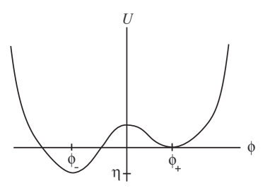
Figure 1: The potential $U$ with the false $(\phi_{+})$ and true $(\phi_{-})$ vacuum

Here $\sigma$ is the surface tension of the wall between the stable and metastable vacua in the limit $\eta\rightarrow 0.$ Thus, according to [10], in this limit the nucleation rate $\Gamma$ is determined by two well defined macroscopic parameters $\eta$ and $\sigma$. Another claim of [10] is that there are no corrections to formula (2) and (3) proportional to powers of the dimensionless parameter $\eta/\sigma^{2}$. Voloshin arrived at these conclusions by an analysis performed in the thin wall approximation. He replaced the original scalar field theory by an effective one, which describes only fluctuations of the critical bubble shape. This approach implies that all other fluctuations of the original scalar field could be properly accounted for by the correct choice of the macroscopic parameters $\eta$ and $\sigma$.

Recently an analytical method was developed [11], which allows one to study nucleation in the scalar field model beyond the thin wall approximation. In [11] this method was used to calculate the nucleation rate for the first order phase transition in the three- dimensional Ginzburg-Landau model. In the present paper we apply the same approach to the two-dimensional case. We calculate the nucleation rate beyond the thin wall approximation and verify directly Voloshin’s claims (2) and (3).

Nucleation theory in two-dimensional scalar field theory has also been studied by Kiselev and Selivanov [12], Strumia and Tetradis [13], and other authors. In these articles, however, different renormalization schemes have been used and $\Gamma$ has not been expressed in terms of macroscopic parameters $\eta$ and $\sigma$. This makes it difficult to compare their results with Voloshin’s claims.

In the article [14] the nucleation rate was calculated in the two-dimensional Ising model in a small magnetic field. If Voloshin’s results (2) and (3) are universal, they should be applicable as well to the Ising model in the critical region. Indeed, expressions (19), (23-26) of [14] rewritten in terms of $\eta$ and $\sigma$ are in a very good agreement with (2), (3). The exponent factors are the same, and the prefactors differ only by the number $\pi^{2}/9\approx 1.0966$, which is very close to unity. This small discrepancy increased our interest in the subject of the present study.

2 Model and notations

We consider the two-dimensional asymmetric Ginzburg-Landau model defined by the Hamiltonian:

$$\mathcal{H}(\phi)=\int\!\!d^{2}x\,\left[\frac{1}{2}(\partial_{\mu}\,\phi(x))^{2}+U(\phi(x))\right],$$ (4)

where $\phi(x)$ is the continuous one-component order parameter, and the potential $U(\phi)$ depicted in Fig. 1 is given by

$$U(\phi)=U_{s}(\phi)+\frac{\eta}{2\,v}(\phi-v)+U_{0}.$$ (5)

Here $U_{s}(\phi)$ denotes the symmetric part of the potential:

$$U_{s}(\phi)=\frac{g}{4!}\left(\phi^{2}-v^{2}\right)^{2}.$$ (6)

The potential $U(\phi)$ has a metastable minimum (false vacuum) at $\phi=\phi_{+}$ and a stable one (true vacuum) at $\phi=\phi_{-}$. The constant term $U_{0}$ in (5) is chosen to ensure $U(\phi_{+})=0$.

The partition function is given by the functional integral

$$Z=\int\!\!D\phi\,\exp\left[-\mathcal{H}(\phi)\right].$$ (7)

The inverse temperature factor has been absorbed into $\mathcal{H}$.

It is convenient to define the mass $m$ and the “inverse temperature” $\beta=1/T$ parameters by

$$m^{2}=\frac{\partial^{2}}{\partial\phi^{2}}U_{s}(\phi)\mid_{\phi=v}=\frac{g\,v^{2}}{3},\qquad\beta=\frac{3m^{2}}{g},$$ (8)

and to introduce dimensionless variables

$$\tilde{x}_{\mu}=\frac{m}{2}\,x_{\mu},\quad\tilde{\eta}=\frac{g}{2\,m^{4}}\,\eta,\quad\varphi(\tilde{x})=\frac{\phi(x)}{v},\quad\varphi_{\pm}=\frac{\phi_{\pm}}{v},\quad\tilde{\mathcal{H}}=\frac{\mathcal{H}}{\beta}.$$ (9)

In dimensionless variables the Hamiltonian and partition function take the form

$$\tilde{\mathcal{H}}(\varphi)=\int\!\!d^{2}\tilde{x}\;\left[\frac{1}{2}\left(\nabla\varphi\right)^{2}+\tilde{U}\left(\varphi(\tilde{x})\right)\right],$$ (10)

where

$$\tilde{U}(\varphi)=\frac{1}{2}\left[\left(\varphi^{2}-1\right)^{2}-\left(\varphi_{+}^{2}-1\right)^{2}\right]+\frac{4}{3}\,\tilde{\eta}\left(\varphi-\varphi_{+}\right),$$ (11)

and

$$Z=\int\!\!D\varphi(\tilde{x})\,\exp\left[-\beta\tilde{\mathcal{H}}(\varphi)\right].$$ (12)

3 The critical bubble solution

The uniform solutions of the field equation

$$\delta\tilde{\mathcal{H}}/\delta\varphi(\tilde{x})=0.$$ (13)

are the stable $\varphi_{-}$ and false (metastable) $\varphi_{+}$ vacua given by

$$\varphi_{\pm}=\pm 1-\frac{\tilde{\eta}}{3}\mp\frac{\tilde{\eta}^{2}}{6}-\frac{4\tilde{\eta}^{3}}{27}+O(\tilde{\eta}^{4}).$$ (14)

The critical bubble $\varphi_{b}(\tilde{x})$ is the non-uniform radially symmetric solution of (13) approaching the false vacuum at infinity. That is,

$$-\frac{d^{2}\varphi_{b}}{d\,\tilde{r}^{2}}-\frac{1}{\tilde{r}}\frac{d\varphi_{b}}{d\,\tilde{r}}+2\varphi_{b}(\varphi_{b}^{2}-1)+\frac{4}{3}\,\tilde{\eta} = 0,$$ (15)

$$\lim_{\tilde{r}\rightarrow\infty}\varphi_{b}(\tilde{r}) = \varphi_{+},$$

where $\tilde{r}=\sqrt{\tilde{x}_{\mu}\,\tilde{x}_{\mu}}.$ The profile of the critical bubble solution is shown schematically in Fig. 2. If $\tilde{\eta}$ is small, the thin wall centered at $\tilde{r}=\tilde{R}$ divides regions of false and stable vacua outside and inside the bubble, respectively.

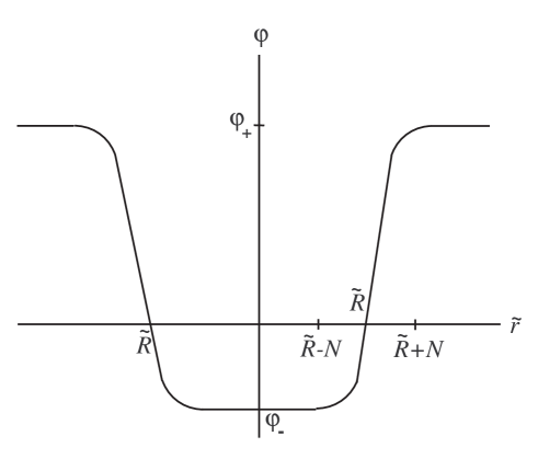
Figure 2: Profile of the critical bubble

Equation (15) can not be solved explicitly. Following the approach introduced by Münster and Rotsch [11] we shall construct the solution by expansion in powers of $\tilde{\eta}$. Introducing the new independent variable $\xi$:

$$\xi=\tilde{r}-\tilde{R},$$ (16)

we write the following series for $\tilde{R}$ and $\varphi_{b}(\xi)$:

$$\tilde{R} = \frac{a_{-1}}{\tilde{\eta}}+a_{0}+a_{1}\tilde{\eta}+a_{2}\tilde{\eta}^{2}+O(\tilde{\eta}^{3}),$$ (17)

$$\varphi_{b}(\xi) = \varphi_{0}(\xi)+\varphi_{1}(\xi)\,\tilde{\eta}+\varphi_{2}(\xi)\tilde{\eta}^{2}+O(\tilde{\eta}^{3}).$$ (18)

After substitution of (16-18) into (15) one obtains perturbatively in $\tilde{\eta}$:

$$a_{-1} = \frac{1}{2},\;a_{0}=0,\;a_{1}=-\frac{2}{9},\;a_{2}=0,$$ (19)

$$\varphi_{0}(\xi) = \tanh\xi,\;\varphi_{1}(\xi)=-\frac{1}{3},$$

$$\varphi_{2}(\xi) = -\frac{1}{24\cosh^{2}\xi}\,\;\biggl{\{}10\xi-16\xi\cosh(2\xi)-2\xi\cosh(4\xi)+$$

$$2\ln\left[2\cosh\xi\right]\left[\xi+8\sinh(2\xi)+\sinh(4\xi)\right]-24\int\limits_{0}^{\xi}\!\!dt\,\,t\tanh t\biggl{\}}.$$

The bubble energy $\tilde{E}=\tilde{\mathcal{H}}\left[\varphi_{b}(x)\right]$ can be written as

$$\tilde{E}=\pi\int\limits_{-\tilde{R}}^{\infty}\!\!d\xi\,(\tilde{R}+\xi)\left(\frac{d\varphi_{b}(\xi)}{d\xi}\right)^{2}.$$ (20)

Substitution of (19) into (20) yields

$$\tilde{E}=2\pi\left[\frac{1}{3\,\tilde{\eta}}+\tilde{\eta}\left(\frac{19}{54}-\frac{\pi^{2}}{9}\right)+O(\tilde{\eta}^{3})\right].$$ (21)

It is the basic principle of homogeneous nucleation theory that the decay of the metastable vacuum occurs through nucleation of the critical bubble. Callan and Coleman expressed the nucleation rate $\Gamma$ of the metastable vacuum in terms of functional determinants [7, 8]. In our notation their result takes the form

$$\tilde{\Gamma}=\frac{\beta\,\tilde{E}}{2\pi}\frac{1}{\sqrt{\left|\lambda_{0}\right|}}\exp\left(-\beta\,\tilde{E}+S\right).$$ (22)

Here $\tilde{\Gamma}=4\Gamma/m^{2}$ is the dimensionless nucleation rate, and the entropy $S$ associated with the critical bubble is given by

$$\exp S=\left[\frac{\det\mathcal{M}^{(0)}}{\det^{\prime}\mathcal{M}}\right]^{1/2},$$ (23)

where $\mathcal{M}$ and $\mathcal{M}^{(0)}$ are the fluctuation operators near the bubble $\varphi_{b}(\tilde{x})$ and metastable uniform vacuum $\varphi_{+}$, respectively:

$$\mathcal{M} = \mathcal{-\partial}^{2}+6\,\left[\varphi_{b}(\tilde{r})\right]^{2}-2,$$ (24)

$$\mathcal{M}^{(0)} = \mathcal{-\partial}^{2}+6\,\varphi_{+}^{2}-2.$$ (25)

The operator $\mathcal{M}$ has two zero modes proportional to $\mathcal{\partial}_{\mu}\,\varphi_{b}(\tilde{x})$, $\mu=1,2,$ and one negative mode with the eigenvalue

$$\lambda_{0}=-4\,\tilde{\eta}^{2}.$$ (26)

The notation $\det^{\prime}$ implies that the three above mentioned modes are omitted in the corresponding determinant. After substitution of (21) and (26), equation (22) simplifies to

$$\tilde{\Gamma}=\frac{\beta}{6\,\tilde{\eta}^{2}}\exp\left(-\,\frac{2\pi\beta}{3\,\tilde{\eta}}+S\right)\left(1+o(\tilde{\eta}^{0})\right).$$ (27)

In the subsequent sections we shall calculate the small $\tilde{\eta}$ expansion for the critical bubble entropy (23) with accuracy $o(\tilde{\eta}^{0})$.

4 The bubble entropy

Let us expand the bubble entropy $S$ into the sum over the angular quantum number $\mu$:

$$S=\sum\limits_{\mu=-\infty}^{\infty}S_{\mu},$$ (28)

where

$$S_{\mu}=\left\{\begin{array}[]{ll}\frac{1}{2}\sum\limits_{j=0}^{\infty}\left(\ln\lambda_{j\mu}^{(0)}-\ln\lambda_{j\mu}\right)&\mbox{for}\ \mu\neq 0,\pm 1\\ \frac{1}{2}\ln\lambda_{0\mu}^{(0)}+\frac{1}{2}\sum\limits_{j=1}^{\infty}\left(\ln\lambda_{j\mu}^{(0)}-\ln\lambda_{j\mu}\right)&\mbox{for}\ \mu=0,\pm 1.\end{array}\right.$$ (29)

Here $\lambda_{j\mu}$ and $\lambda_{j\mu}^{(0)}$ are the eigenvalues of the radial Schrödinger operators corresponding to $\mathcal{M}$ and $\mathcal{M}^{(0)}$:

$$H_{\mu} = -\frac{d^{2}}{d\,\tilde{r}^{2}}-\frac{1}{\tilde{r}}\frac{d}{d\,\tilde{r}}+\frac{\mu^{2}}{\tilde{r}^{2}}+6\,\left[\varphi_{b}(\tilde{r})\right]^{2}-2,$$ (30)

$$H_{\mu}^{(0)} = -\frac{d^{2}}{d\,\tilde{r}^{2}}-\frac{1}{\tilde{r}}\frac{d}{d\,\tilde{r}}+\frac{\mu^{2}}{\tilde{r}^{2}}+6\,\varphi_{+}^{2}-2,$$ (31)

$$H_{\mu}\ \psi_{j\mu}(\tilde{r}) = \lambda_{j\mu}\ \psi_{j\mu}(\tilde{r}),\qquad H_{\mu}^{(0)}\chi_{j\mu}(\tilde{r})=\lambda_{j\mu}^{(0)}\chi_{j\mu}(\tilde{r}).$$

The eigenfunctions $\psi_{j\mu},\ \chi_{j\mu}$ are supposed to be finite at the origin $\tilde{r}=0$ and to obey the zero boundary condition at some large $L:\psi_{j\mu}(L)=\chi_{j\mu}(L)=0.$

4.1 Calculation of the “partial” entropy $S_{\mu}$

Let us first consider the case $\mu\neq 0,\pm 1.$ For such a $\mu$ the operators $H_{\mu}$ and $H_{\mu}^{(0)}$ are positive. Therefore the “partial” entropy $S_{\mu}$ can be written in terms of the trace of the resolvent operators:

$$S_{\mu}=\frac{1}{2}\int\limits_{C_{1}}\frac{d\lambda}{2\pi i}\ A(\lambda,\mu)\ \ln\lambda,$$ (32)

where

$$A(\lambda,\mu)=\mbox{Sp}\left[\left(\lambda-H_{\mu}\right)^{-1}-\left(\lambda-H_{\mu}^{(0)}\right)^{-1}\right].$$

The integration path $C_{1}$ shown in Fig. 3 lies in the right complex half-plane of $\lambda$ and goes around the spectra of both operators $H_{\mu}$ and $H_{\mu}^{(0)}$ in the clockwise direction. It should be noted that the representation (32) is valid also for $\mu=0,\pm 1$. In the latter case the lowest discrete mode $\lambda_{0\mu}\leq 0$ becomes negative ($\mu=0$) or zero ($\mu=\pm 1$). These modes contribute neither to (29) nor to (32).

After deformation of the path $C_{1}$ into the path $C_{2}$ which goes around the logarithmic cut positioned at the negative real axis (see Fig. 3), one obtains

$$S_{\mu}=-\frac{1}{2}\int\limits_{-\infty}^{0}\!\!d\lambda\ A(\lambda,\mu).$$ (33)

In this equation one can proceed to the thermodynamic limit $L\rightarrow\infty$.

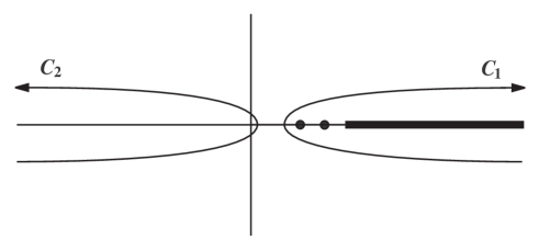
Figure 3: Integration paths $C_{1}$ and $C_{2}$ in the complex $\lambda$-plane

We obtained an exact representation for the integrand in (33). To describe it some notations are necessary.

Let $f_{i}(\tilde{r},\lambda),\ g_{i}(\tilde{r},\lambda),\ i=1,2$ be the solutions of the linear ordinary differential equation

$$H_{\mu}\ \psi(\tilde{r})=\lambda\ \psi(\tilde{r})$$ (34)

determined by their asymptotics:

$$f_{1}(\tilde{r},\lambda) \rightarrow K_{\mu}(q\tilde{r}),\ \mbox{and}\ f_{1}(\tilde{r},\lambda)\rightarrow I_{\mu}(q\tilde{r}),\ \mbox{at}\ \tilde{r}\rightarrow\infty,$$ (35)

$$g_{1}(\tilde{r},\lambda) \rightarrow K_{\mu}(q_{-}\,\tilde{r}),\ \mbox{and}\ g_{1}(\tilde{r},\lambda)\rightarrow I_{\mu}(q_{-}\,\tilde{r}),\ \mbox{at}\ \tilde{r}\rightarrow 0.$$ (36)

Here $K_{\mu}(z)$ and $I_{\mu}(z)$ are the modified Bessel functions, the parameters $q$ and $q_{-}$ are defined as:

$$q=\left(6\varphi_{+}^{2}-\lambda-2\right)^{1/2},\quad q_{-}=\left(6\varphi_{-}^{2}-\lambda-2\right)^{1/2}.$$ (37)

Since the second order equation (34) has two linearly independent solutions, there is a linear dependence between the functions $g_{i}(\tilde{r},\lambda)$ and $f_{i}(\tilde{r},\lambda)$:

$$g_{i}(\tilde{r},\lambda)=\sum\limits_{j=1,2}\alpha_{ij}(\lambda)\ f_{j}(\tilde{r},\lambda).$$ (38)

The above relation defines the $2\times 2$-matrix $\alpha(\lambda)$. The integrand in (33) can be expressed explicitly in terms of this matrix:

$$A(\lambda,\mu)=\frac{3\mu(\varphi_{+}^{2}-\varphi_{-}^{2})}{(\lambda+2-6\varphi_{-}^{2})(\lambda+2-6\varphi_{+}^{2})}+\frac{d\ln\alpha_{22}(\lambda)}{d\lambda},$$ (39)

where $\lambda$ is assumed to be real and negative.

The representation (39) for the trace of resolvent operators is exact. However, equation (34) can not be solved in closed form for arbitrary $\tilde{\eta}$. So we have to consider the small-$\tilde{\eta}$ expansion for $\alpha_{22}(\lambda)$. We have obtained two terms of this expansion by use of a perturbation theoretical analysis of the scattering problem (34 – 38). Omitting the details, the logarithmic derivative of the matrix element $\alpha_{22}(\lambda)$ up to quadratic terms in $\tilde{\eta}$ takes the form:

$$\frac{d\ln\alpha_{22}(\lambda)}{d\lambda}=\frac{1}{(4+p^{2}-\lambda)^{1/2}}\left[\frac{2\,p^{2}}{\left(\lambda-4\right)^{2}}-\frac{1}{\lambda-4}+\frac{1}{\lambda-3-p^{2}}+\frac{2}{\lambda-p^{2}}\right]+O(\tilde{\eta}^{2}).$$ (40)

Here $p$ is the angular momentum parameter defined as $p=2\,\tilde{\eta}\mu\approx\tilde{R}\,\mu$, which is considered to be a quantity of order 1 for later purposes.

Substitution of (40) and (14) into (39) yields:

$$A(\lambda,\mu) = \frac{1}{\left(4+p^{2}-\lambda\right)^{1/2}}\left[\frac{2\,p^{2}}{\left(\lambda-4\right)^{2}}-\frac{1}{\lambda-4}+\frac{1}{\lambda-3-p^{2}}+\frac{2}{\lambda-p^{2}}\right]$$ (41)

$$-\frac{2\,\left|p\right|}{\left(\lambda-4\right)^{2}}+O(\tilde{\eta}^{2}).$$

Integrating (33) we obtain the “partial” entropy $S_{\mu}$:

$$S_{\mu}=\frac{\left|p\right|}{4}-\frac{\left(p^{2}+4\right)^{1/2}}{4}+\frac{1}{2}\ln\left\{\frac{\left[\left(p^{2}+4\right)^{1/2}+2\right]^{2}}{p^{2}}\,\cdot\frac{(p^{2}+4)^{1/2}+1}{(p^{2}+4)^{1/2}-1}\right\}.$$ (42)

4.2 Summation of the $\mu$-series

Expression (42) has a logarithmic singularity at $p=0$. This singularity arises from the lowest discrete level of the Hamiltonian (31). To account for the contribution of this level properly, let us rewrite (28) as

$$S=\sum\limits_{\mu=-\infty}^{\infty}\mbox{}s_{\mu}(z)+\ln R(z),$$ (43)

where

$$s_{\mu}(z)=\frac{\left|p\right|}{4}-\frac{\left(p^{2}+4\right)^{1/2}}{4}+\frac{1}{2}\ln\left\{\frac{\left[(p^{2}+4)^{1/2}+2)\right]^{2}}{p^{2}+z^{2}}\,\cdot\frac{(p^{2}+4)^{1/2}+1}{(p^{2}+4)^{1/2}-1}\right\},$$ (44)

$$\ln R(z)=\frac{1}{2}\sum\limits_{\mu=-\infty}^{\infty}\ln\frac{p^{2}+z^{2}}{p^{2}},$$ (45)

and $z$ is some fixed positive number.

First, we shall determine $R(z).$ Taking into account the presence of the negative and zero modes, the following corrections are necessary:

$$\ln R(z) = \frac{1}{2}\sum\limits_{\mu=-\infty}^{\infty}\ln\frac{p^{2}+z^{2}}{p^{2}}=\frac{1}{2}\sum\limits_{\mu=-\infty}^{\infty}\ln\frac{4\,\tilde{\eta}^{2}\mu^{2}+z^{2}}{4\,\tilde{\eta}^{2}\mu^{2}}\longrightarrow$$ (46)

$$\frac{1}{2}\sum\limits_{\mu=-\infty\atop\mu\neq 0,\pm 1}^{\infty}\ln\frac{4\,\,\tilde{\eta}^{2}\,\mu^{2}+z^{2}}{4\,\tilde{\eta}^{2}(\mu^{2}-1)}+\frac{1}{2}\ln z^{2}+\ln(z^{2}+4\,\tilde{\eta}^{2}).$$

These corrections arise from two facts:

1. The logarithmic singularity of (42) at $p\rightarrow 0$ comes from the first discrete level $\lambda_{0\mu}=4\tilde{\eta}^{2}(\mu^{2}-1)$ of the operator (30).

2. The three eigenvalues $\lambda_{0}=-4\tilde{\eta}^{2},\ \lambda_{\pm 1}=0$ of the operator (30) already accounted for in (27) should be omitted in $S$ and $\ln R(z).$

After these corrections we obtain from (46)

$$R(z)=z\,\left(z^{2}+4\tilde{\eta}^{2}\right)\prod\limits_{\mu=2}^{\infty}\frac{\mu^{2}+(z/2\tilde{\eta})^{2}}{\mu^{2}-1}=\left(2\tilde{\eta}\right)^{3}\frac{z}{2\tilde{\eta}}\left(1+\frac{z^{2}}{4\tilde{\eta}^{2}}\right)\ f(\frac{z}{2\tilde{\eta}}),$$

where

$$f(x)=\prod\limits_{\mu=2}^{\infty}\frac{\mu^{2}+x^{2}}{\mu^{2}-1}=\frac{2}{\pi}\frac{\sinh\left(\pi x\right)}{x(x^{2}+1)}.$$

Therefore,

$$R(z)=\frac{2}{\pi}\left(2\tilde{\eta}\right)^{3}\sinh\left(\pi\frac{z}{2\tilde{\eta}}\right)\cong\frac{1}{\pi}\left(2\tilde{\eta}\right)^{3}\exp\left(\frac{z\pi}{2\tilde{\eta}}\right),$$

since $\tilde{\eta}$ is small, and $z$ is a fixed number. Thus, we obtain

$$\ln R(z)=3\ln\left(2\tilde{\eta}\right)-\ln\pi+\frac{z\pi}{2\tilde{\eta}}.$$ (47)

This result can also be obtained by the $\zeta$-function technique described in [11].

For the calculation of the first sum in the right-hand side of (43) it is convenient to apply Poisson’s summation formula:

$$\sum\limits_{\mu=-\infty}^{\infty}s_{\mu}(z)=\sum\limits_{k=-\infty}^{\infty}\ \int\limits_{-\infty}^{\infty}\!\!d\mu\ s_{\mu}(z)\exp\left(2\pi i\mu k\right).$$ (48)

The integrals in terms with $k\neq 0$ on the right-hand side converge. One can easily show that these integrals (at $k\neq 0$) are of order $\tilde{\eta}$ and can therefore be neglected in the adopted approximation. So, it is sufficient to calculate the $k=0$ term only, which we denote by $s(z)$. Straightforward calculations yield:

$$s(z)=s(0)-\frac{\pi z}{2\,\tilde{\eta}}=\int\limits_{-\,\infty}^{\infty}\!\!d\mu\ S_{\mu}-\frac{\pi z}{2\,\tilde{\eta}},$$ (49)

where $S_{\mu}$ is given by (42).

Now we can substitute (49) and (47) into (43) and obtain

$$\exp S=\frac{\left(2\,\tilde{\eta}\right)^{3}}{\pi}\exp S^{(-1)}\left[1+o(\tilde{\eta}^{0})\right],$$ (50)

where

$$S^{(-1)}\equiv\int\limits_{-\,\infty}^{\infty}\!\!d\mu\ S_{\mu}\sim\tilde{\eta}^{-1}.$$

As $p\rightarrow\infty,$ $S_{\mu}\sim-(2p)^{-1}.$ Therefore the integral in $\mu$ on the right-hand side diverges logarithmically at large $\left|\mu\right|$. Indeed, this is the well-known ultraviolet divergency. Introducing a cut-off $p_{m}$ in $\left|p\right|$ one finds:

$$S^{(-1)}\leadsto\int\limits_{-\,p_{m}}^{p_{m}}\!\frac{dp}{2\,\tilde{\eta}}\ S_{\mu}=\frac{1}{2\,\tilde{\eta}}\left(5\ln p_{m}+\frac{11}{2}-\frac{\pi}{\sqrt{3}}\right).$$ (51)

Relations (50), (51) are our final results for the bubble entropy.

5 Decay rate

Substitution of (50) into (27) yields for the dimensionless decay rate $\tilde{\Gamma}$:

$$\tilde{\Gamma}=\frac{4\beta\,\tilde{\eta}}{3\pi}\,\exp\left(-\,\beta E(\tilde{\eta},T)\right),$$ (52)

where

$$E(\tilde{\eta},T) = \frac{2\pi}{3\,\tilde{\eta}}-T\ \Delta S^{(-1)}+\,o(\tilde{\eta}^{0})$$

$$= \frac{1}{\tilde{\eta}}\,\left(\frac{2\pi}{3}-\frac{T}{2}(5\ln p_{m}+\frac{11}{2}-\frac{\pi}{\sqrt{3}})\right)+\,o(\tilde{\eta}^{0}).$$

To compare (52), (5) with Voloshin’s result (2), (3), let us rewrite the latter in the dimensionless variables (9) for the model (10)–(12):

$$\tilde{\Gamma}=\frac{4\beta\,\tilde{\eta}\,\langle\varphi\rangle}{3\pi}\,\exp\left[-\,\,\frac{3\pi\,\tilde{\sigma}^{2}\,\beta}{8\,\tilde{\eta}\,\langle\varphi\rangle}\right],$$ (54)

where $\tilde{\sigma}$ is the surface tension, and $\langle\varphi\rangle$ is the average value of the scalar order parameter at $\tilde{\eta}=0.$ In (54) we have replaced the energy difference between the false and true vacua by $\frac{8}{3}\,\tilde{\eta}\,\langle\varphi\rangle\,\beta$.

It should be stressed that the parameters $\langle\varphi\rangle$ and $\tilde{\sigma}$ in (54) are exact macroscopic quantities which depend on the interaction parameter $g$, or in other terms, on the “temperature” $T\equiv\beta^{-1}=g/(3m^{2})$. At low “temperatures” these quantities can be expanded in $T$:

$$\langle\varphi\rangle=1+T\,\rho+O(T^{\,2}),\quad\tilde{\sigma}=\frac{4}{3}+T\,\vartheta+O(T^{\,2}),$$ (55)

and the corrections linear in $T$ can be found perturbatively:

$$\rho = -\frac{3}{4\pi}\left(\frac{1}{2}+\ln p_{m}\right),$$ (56)

$$\vartheta = -\frac{3\ln p_{m}}{\pi}-\frac{3}{\pi}+\frac{1}{2\sqrt{3}}.$$ (57)

Here $\vartheta$ is the one-loop correction in $\langle\varphi\rangle$, the correction in $\tilde{\sigma}$ was calculated in the strip geometry from the ratio of partition functions $\beta\tilde{\sigma}=L_{2}^{-1}\ln(Z_{0}/Z_{1})$ with different boundary conditions:

$$Z_{0} : \quad\varphi(\tilde{x}_{1}+L_{1},\tilde{x}_{2})=\varphi(\tilde{x}_{1},\tilde{x}_{2}+L_{2})=\varphi(\tilde{x}_{1},\tilde{x}_{2}),$$

$$Z_{1} : \quad-\varphi(\tilde{x}_{1}+L_{1},\tilde{x}_{2})=\varphi(\tilde{x}_{1},\tilde{x}_{2}+L_{2})=\varphi(\tilde{x}_{1},\tilde{x}_{2}).$$

It should be noted that both $\rho$ and $\vartheta$ contain logarithmic ultraviolet divergencies and depend on the cut-off procedure. In (56), (57) we have chosen a similar cut-off-procedure as in (51). Substituting (55)–(57) into (54) and expanding in $T$ one obtains

$$\tilde{\Gamma}=\frac{4\beta\,\tilde{\eta}}{3\pi}\,\exp\left[-\frac{2\pi}{3\,T\,\tilde{\eta}}+\frac{1}{2\,\tilde{\eta}}\left(5\ln p_{m}+\frac{11}{2}-\frac{\pi}{\sqrt{3}}+O(T)\right)\right]$$

in agreement with our results (52), (5).

Summary: Our semiclassical calculation of the nucleation rate $\Gamma$ in the two-dimensional Landau-Ginzburg $\phi^{4}$-model confirms Voloshin’s results (2), (3), which were derived in the thin wall approximation. In particular, we confirm the prefactor value $\mathcal{A}=\eta/(2\pi)$ first obtained by Kiselev and Selivanov [12], and Voloshin [10].

This value differs from that obtained for the two dimensional critical Ising model [14] by the numerical factor $\pi^{2}/9\approx 1.0966$. We suppose that this small discrepancy is the result of approximations used in [14], and the prefactor value $\mathcal{A}=\eta/(2\pi)$ is universal.

Acknowledgments

One of us (S.B. R.) would like to thank the Institute of Theoretical Physics of the University of Münster for hospitality. This work is supported by the Deutsche Forschungsgemeinschaft (DFG) under grant GRK 247/2-99 and by the Fund of Fundamental Investigations of Republic of Belarus.

References

- [1] P.A. Rikvold and B.M. Gorman, in Annual Review of Computational Physics I, D. Stauffer (ed.), World Scientific, Singapore, 1994
- [2] H.E. Stanley, Introduction to Phase Transitions and Critical Phenomena, Clarendon Press, Oxford, 1971
- [3] A.H. Guth, The Inflationary Universe, Addison Wesley, Reading, Mass., 1997
- [4] H.A. Kastrup, Phys. Letters B 419 (1998) 40
- [5] J.S. Langer, Ann. Phys. (N.Y.) 41 (1967) 108
- [6] M.B. Voloshin, I.Yu. Kobzarev and L.B. Okun’, Yad. Fiz. 20 (1974) 1229 [Sov. J. Nucl. Phys. 20 (1975) 644]
- [7] S. Coleman, Phys. Rev. D15 (1977) 2929, Erratum: Phys. Rev. D16 (1977) 1248
- [8] C.G. Callan and S. Coleman, Phys. Rev. D16 (1977) 1762
- [9] A.D. Linde, Nucl. Phys. B 216 (1983) 421
- [10] M.B. Voloshin, Yad. Fiz. 42 (1985) 1017 [Sov. J. Nucl. Phys. 42 (1985) 644 ]
- [11] G. Münster and S. Rotsch, Eur. Phys. J. C 12 (2000) 161
- [12] V.G. Kiselev and K.G. Selivanov, Pis’ma Zh. Eksp. Teor. Fiz. 39 (1984)72 [JETP Lett. 39 (1984) 72 ]
- [13] A. Strumia and N. Tetradis, Nucl.Phys. B 560 (1999) 482
- [14] S.B. Rutkevich, Phys. Rev. B 60 (1999) 14525