Many-body Green’s function theory for the magnetic reorientation of thin ferromagnetic films

Abstract

The field-induced reorientation of the magnetization of ferromagnetic films is treated within the framework of many-body Green’s function theory by considering all components of the magnetization. We present a new method for the calculation of expectation values in terms of the eigenvalues and eigenvectors of the equations of motion matrix for the set of Green’s functions. This formulation allows a straightforward extension of the monolayer case to thin films with many layers and for arbitrary spin and moreover provides a practicable procedure for numerical computation. The model Hamiltonian includes a Heisenberg term, an external magnetic field, a second-order uniaxial single-ion anisotropy, and the magnetic dipole-dipole coupling. We utilize the Tyablikov (RPA) decoupling for the exchange interaction terms and the Anderson-Callen decoupling for the anisotropy terms. The dipole coupling is treated in the mean-field approximation, a procedure which we demonstrate to be a sufficiently good approximation for realistic coupling strengths. We apply the new method to monolayers with spin $S\geq 1$ and to multilayer systems with $S=1$. We compare some of our results to those where mean-field theory (MFT) is applied to all interactions, pointing out some significant differences.

1 Introduction

In this paper, we extend our earlier investigations EFJK99 ; FJK00 on the reorientation of the magnetization of a ferromagnetic monolayer with spin $S=1$ to multilayer systems with arbitrary spin, $S$. The components of the magnetization as functions of temperature and film thickness are calculated within the framework of a many-body Green’s function theory, allowing the direct calculation of the magnetic orientation. Furthermore, we derive and apply a non-perturbative expression for the temperature dependence of the second-order single-ion anisotropy by minimizing the free energy with respect to this orientation angle.

For convenience, mean-field theory (MFT) is often applied to such problems, either by diagonalisation of a single-particle Hamiltonian JeB98 , or by a thermodynamic perturbation theory theo . We emphasize that this approximation completely neglects collective excitations (spin waves) which are known to have a much greater influence on the magnetic properties of 2D systems than on 3D bulk properties. In fact, recent calculations on a trilayer system Je99 demonstrate that MFT is incapable of accounting for the induced magnetization observed in coupled layers unless an unrealistically large interlayer coupling is postulated. On the other hand, the many-body Green’s function techniques, which take the collective excitations approximately into account, can explain the experimental observations assuming an interlayer exchange coupling of reasonable size. We point out that the dependence of the magnetization and the Curie temperature on the film thickness has also been studied within Green’s function theory SN99 . Also, in references Bru91 and SW92 Green’s function techniques are applied to magnetization problems. However, in all these references only a single component of the magnetization is considered. Therefore, a reorientation of the magnetization as a function of temperature, film thickness, or magnetic field cannot be calculated. A reorientation of the magnetization is considered in reference EM91 , where Green’s functions are used after a Holstein-Primakoff mapping of the spin operators to bosons. In order to solve the non-Hermitian eigenvalue problem, right and left eigenvectors are applied for its solution, similar to what is done in the present paper. The theory is, however, only valid at low temperatures. Another method for the treatment of the magnetic reorientation for all temperatures is a Schwinger-Boson theory Timm00 , as an alternative to the Green’s function method of this paper.

In the present work, we treat the field-induced reorientation of the magnetization for all temperatures of interest. Since expectation values of all three components of the spin operator are considered, a corresponding set of Green’s functions must be defined. We introduce a new method for the calculation of the expectation values, which utilizes not only the eigenvalues but also the eigenvectors of the (non-symmetric) matrix governing the equations of motion for the Green’s functions. This formulation is more compact than the usual one FJK00 and, most importantly, suggests a practicable way of treating the multilayer case for arbitrary spin. We make no attempt to go beyond the Tyablikov (Random Phase Approximation: RPA) decoupling for the exchange terms, since we have shown in reference EFJK99 that this decoupling scheme for a monolayer with spin $S=1/2$ compares well indeed with an ‘exact’ Quantum Monte Carlo (QMC) calculation. The single-ion anisotropy term is decoupled with the Anderson-Callen method AC64 , because, as shown in FJK00 , other single-ion decoupling schemes, e.g. that of Lines Lin67 , lead to difficulties when calculating the magnetic reorientation. Furthermore, we include the magnetic dipole coupling, which is treated within a simplified (non-dispersive) approximation, which corresponds to its mean field treatment. The dipole coupling was not considered in our earlier work FJK00 , which was restricted to the case of a monolayer with spin $S=1$.

The paper is organized as follows. In Section 2 the Green’s function formalism is outlined. The eigenvector method is then presented for the monolayer case and it is shown that this leads to a transparent extension to the case of many layers. Section 3 deals with the results. First the effect of the dipole coupling on the magnetic reorientation is discussed using the monolayer with spin $S=1$ as an example. Secondly, we discuss monolayers with spins $S>1$. Thirdly the formalism is applied to the case of many layers. Finally Section 4 contains a discussion of the results and an outlook for further investigations. In Appendix A, different approximations for the magnetic dipole coupling are investigated. Details of the formalism for $S>1$ are derived in Appendix B.

2 The Green’s function formalism

In order to study the field-induced magnetic reorientation of a ferromagnetic thin film we investigate a spin Hamiltonian consisting of an isotropic Heisenberg exchange interaction, $J_{kl}$, between nearest neighbour lattice sites, a second-order single-ion lattice anisotropy with strength, $K_{2,k}$, the magnetic dipole coupling with strength, $g_{kl}$, and an external magnetic field, ${\bf{B}}=(B^{x},B^{y},B^{z})$,

$${\cal H} = -\frac{1}{2}\sum_{<kl>}J_{kl}\;{\bf S}_{k}\cdot{\bf S}_{l}-\sum_{k}K_{2,k}(S_{k}^{z})^{2}$$

$$-\sum_{k}\Big{(}\frac{1}{2}B^{-}S_{k}^{+}+\frac{1}{2}B^{+}S_{k}^{-}+B^{z}S_{k}^{z}\Big{)}$$

$$+\frac{1}{2}\sum_{kl}\frac{g_{kl}}{r_{kl}^{5}}\Big{(}r_{kl}^{2}\,{\bf S}_{k}\cdot{\bf S}_{l}-3({\bf S}_{k}\cdot{\bf r}_{kl})({\bf S}_{l}\cdot{\bf r}_{kl})\Big{)}\;.$$

Here the notation $S_{i}^{\pm}=S_{i}^{x}\pm iS_{i}^{y}$ and $B^{\pm}=B^{x}\pm iB^{y}$ is introduced, $k$ and $l$ are lattice site indices, and $\langle kl\rangle$ indicates summation over nearest neighbours only. Each layer is assumed to be ferromagnetically ordered (collinear magnetization), whereas the magnetization of different layers need not to be collinearly aligned. Furthermore, inhomogeneous systems can be considered which are characterized by different layer-dependent coupling constants and magnetic moments. We do not include a fourth order uniaxial anisotropy term, $-\sum_{k}K_{k,4}(S_{k}^{z})^{4}$, because it is difficult to find a proper decoupling of this term in the equations of motion for the Green’s functions. This means that the formalism of the present paper is only adequate for the physical situation in which such a term is of no importance.

As in reference FJK00 , we introduce the set of thermal Green’s functions in the spectral representation

$$G_{ij(\eta)}^{\alpha,mn}(\omega)=\langle\langle S_{i}^{\alpha};(S_{j}^{z})^{m}(S_{j}^{-})^{n}\rangle\rangle_{\omega}\;;\ \ \alpha=+,-,z\ \ ,$$ (2)

where $\omega$ denotes the energy, and $\eta=\pm 1$ refers to the commutator ($\eta=-1$) or anti-commutator ($\eta=+1$) Green’s functions, respectively; $n\geq 1$ and $m\geq 0$ are integers, $i$ and $j$ denote lattice sites. In order to obtain a closed set of equations of motion for the Green’s functions, we treat the exchange term by a generalized Tyablikov (RPA) Tya67 decoupling, and the anisotropy term by the Anderson-Callen decoupling AC64 .

In our previous work the corresponding thermal correlation functions

$$C_{ij}^{mn,\alpha}=\langle(S^{z}_{j})^{m}(S^{-}_{j})^{n}S_{i}^{\alpha}\rangle$$ (3)

have been obtained by applying the spectral theorem Tya67 . Because of vanishing eigenvalues it is important to use the spectral theorem including the term obtained from the anti-commutator Green’s functions

$$D^{mn}_{ij}=\frac{1}{2}\lim_{\omega\to 0}G_{ij(\eta=+1)}^{mn}\,.$$ (4)

Together with the so-called regularity conditions, which are derived from the fact that the spectral representation of the commutator Green’s function must be regular for $\omega=0$, we have derived a set of coupled equations for the correlation functions. The solution yields the components of the magnetization, thus determining directly the reorientation angle of the magnetization induced by the applied external field. In the present paper, we rederive these equations by a method which utilizes the eigenvectors as well as the eigenvalues of the matrix determining the Green’s functions. This more compact formulation furnishes a practicable way to treat the multilayer case and general spin quantum numbers $S$. It is didactically advantageous to demonstrate this new method first for a monolayer; the generalization to the multilayer case then follows in a straightforward and transparent way.

2.1 The eigenvector method for the monolayer

The equations of motion for the Green’s functions in the spectral representation read

$$\omega\;G_{ij(\eta)}^{\alpha,mn}(\omega)=A_{ij(\eta)}^{\alpha,mn}+\langle\langle[S_{i}^{\alpha},{\cal H}]_{-1};(S_{j}^{z})^{m}(S_{j}^{-})^{n}\rangle\rangle\,,$$ (5)

with the inhomogeneities

$$A_{ij(\eta)}^{\alpha,mn} = \langle[S_{i}^{\alpha},(S_{j}^{z})^{m}(S_{j}^{-})^{n}]_{\eta}\rangle$$ (6)

$$= \langle S_{i}^{\alpha}(S_{j}^{z})^{m}(S_{j}^{-})^{n}+\eta(S_{j}^{z})^{m}(S_{j}^{-})^{n}S_{i}^{\alpha}\rangle\,,$$

where $\langle\cdots\rangle={\rm Tr}(\cdots e^{-\beta\cal{H}})$ with $\beta=1/k_{B}T$ and $k_{B}$ Boltzmann’s constant, and $\eta=+1$ or $-1$, respectively.

The higher Green’s functions in equation (5) due to the exchange interaction term are decoupled by a generalized Tyablikov (RPA) decoupling Tya59

$$\langle\langle S_{i}^{\alpha}S_{k}^{\beta};(S_{j}^{z})^{m}(S_{j}^{-})^{n}\rangle\rangle\simeq\langle S_{i}^{\alpha}\rangle\;G_{kj}^{\beta,mn}+\langle S_{k}^{\beta}\rangle\;G_{ij}^{\alpha,mn}\;.$$ (7)

In reference FJK00 the proper inclusion of the single-ion anisotropy with Green’s function techniques was thoroughly discussed in connection with the magnetic reorientation. Accordingly, we choose the Anderson-Callen AC64 ; FJK00 decoupling for the treatment of the anisotropy terms:

$$\langle\langle S_{i}^{\pm}S_{i}^{z}+S_{i}^{z}S_{i}^{\pm}\rangle\rangle$$

$$\simeq 2\langle S_{i}^{z}\rangle\Big{(}1-\frac{1}{2S^{2}}[S(S+1)-\langle S_{i}^{z}S_{i}^{z}\rangle]\Big{)}G_{ij}^{\pm,mn}\,.$$ (8)

Because we are interested in laterally periodic systems we perform a Fourier transformation to the two-dimensional wave vector space ${\bf k}$. Introducing vectors for the Green’s functions, ${\bf G}_{\eta}^{mn}({\bf k},\omega)$, and for the inhomogeneities, ${\bf A}_{\eta}^{mn}$,

$${\bf G}_{\eta}^{mn}({\bf{k},\omega})=\left(\begin{array}[]{c}G_{\eta}^{+,mn}({\bf{k}},\omega)\\ G_{\eta}^{-,mn}({\bf{k}},\omega)\\ G_{\eta}^{z,mn}({\bf{k}},\omega)\end{array}\right)\,,\hskip 8.5359pt{\bf A}_{\eta}^{mn}=\left(\begin{array}[]{c}A_{\eta}^{+,mn}\\ A_{\eta}^{-,mn}\\ A_{\eta}^{z,mn}\end{array}\right)\,,$$ (9)

the equations of motion, which are derived in detail in reference FJK00 , can be written in a compact form

$$(\omega\,{\bf 1}-{\bf\Gamma})\;{\bf G}_{\eta}^{mn}={\bf A}_{\eta}^{mn},$$ (10)

where 1 is the unit matrix and the non-symmetric matrix ${\bf\Gamma}$ is given by

$${\bf\Gamma}=\left(\begin{array}[]{@{\hspace*{3mm}}c@{\hspace*{5mm}}c@{\hspace*{5mm}}c@{\hspace*{3mm}}}\hskip 8.53581pt\lx@intercol\hfil\;\;\;\;\tilde{H^{z}}\hfil\hskip 14.22636pt&0\hfil\hskip 14.22636pt&-H^{+}\hfil\hskip 8.53581pt\\ \hskip 8.53581pt\lx@intercol\hfil 0\hfil\hskip 14.22636pt&-\tilde{H^{z}}\hfil\hskip 14.22636pt&\;\;\;H^{-}\hfil\hskip 8.53581pt\\ \hskip 8.53581pt\lx@intercol\hfil-\frac{1}{2}H^{-}\hfil\hskip 14.22636pt&\;\frac{1}{2}H^{+}\hfil\hskip 14.22636pt&0\hfil\hskip 8.53581pt\end{array}\right)\;,$$ (11)

with the abbreviations

$$H^{\alpha} = B^{\alpha}+\langle S^{\alpha}\rangle\,J\,(q-\gamma_{\bf k})\,,\qquad\alpha=+,-,z\,,$$

$$\tilde{H}^{z} = H^{z}+K_{2}\,\Phi\;=\;Z+\langle S^{z}\rangle\,J\,(q-\gamma_{\bf k})\,,$$

$$Z = B^{z}+K_{2}\,\Phi\,,$$ (12)

$$\Phi = 2\langle S^{z}\rangle\Big{(}1-\frac{1}{2S^{2}}[S(S+1)-\langle S^{z}S^{z}\rangle]\Big{)}\;.$$

For a square lattice with a lattice constant taken to be unity, one obtains $\gamma_{\bf k}=2(\cos k_{x}+\cos k_{y})$, and $q=4$ is the number of nearest neighbours. Note that ${\bf A}_{\eta}^{mn}={\bf A}_{\eta}^{mn}({\bf k})$ depends on the wave vector ${\bf k}$ for $\eta=1$ but not for $\eta=-1$.

Similar to the exchange coupling, the long-range dipole coupling also induces a momentum dependence into the magnon dispersion relation $\omega({\bf k})$. Due to the oscillating lattice sums the consideration of the k- dependence of this coupling obtained e.g. in RPA is fairly complicated and time consuming. Therefore we accept for the present calculations an approximate description of the dipole coupling in the dispersion relation, in particular its k- dependent terms are neglected, which is equivalent to its mean field approximation. In Appendix A, we show that for dipole interactions small compared to the exchange coupling, which is the case for the ferromagnetic $3d$- transition metals, this approximation is satisfactory. The approximation of Appendix A merely leads to a renormalization of the external magnetic field components $B^{\pm}$ and $B^{z}$, which for the $i$th atomic layer in the case of a multilayer with $N$ layers reads

$$B^{\pm}_{i} \to B^{\pm}+\sum_{j=1}^{N}\;g_{ij}\;\langle S_{j}^{\pm}\rangle\;T^{|i-j|}\;,$$

$$B^{z}_{i} \to B^{z}-2\sum_{j=1}^{N}\;g_{ij}\;\langle S_{j}^{z}\rangle\;T^{|i-j|}\;,$$ (13)

where the lattice sums for a two-dimensional square lattice are given by ($n=|i-j|$)

$$T^{n}=\sum_{lm}\frac{l^{2}-n^{2}}{(l^{2}+m^{2}+n^{2})^{5/2}}\;.$$ (14)

The indices ($lm$) run over all sites of the square $j$-th layer, excluding the terms with $l^{2}+m^{2}+n^{2}=0$. For the monolayer ($N=1$) one has $i=j$, and one obtains in particular $T^{0}\simeq 4.5165$. As can be seen from equations (13), the dipole coupling reduces the effect of the external field component in $z$-direction and enhances the effect of the transversal field components $B^{\pm}$.

We now introduce a transformation which diagonalizes the matrix ${\bf\Gamma}$

$${\bf L\;\Gamma\;R}={\bf\Omega}=\left(\begin{array}[]{@{\hspace*{3mm}}c@{\hspace*{5mm}}c@{\hspace*{5mm}}c@{\hspace*{3mm}}}\hskip 8.53581pt\lx@intercol\hfil\omega_{0}\hfil\hskip 14.22636pt&0\hfil\hskip 14.22636pt&0\hfil\hskip 8.53581pt\\ \hskip 8.53581pt\lx@intercol\hfil 0\hfil\hskip 14.22636pt&\omega_{+}\hfil\hskip 14.22636pt&0\hfil\hskip 8.53581pt\\ \hskip 8.53581pt\lx@intercol\hfil 0\hfil\hskip 14.22636pt&0\hfil\hskip 14.22636pt&\omega_{-}\hfil\hskip 8.53581pt\end{array}\right)\;,$$ (15)

where the eigenvalues turn out to be $\omega_{0}=0,\ \omega_{\pm}=\pm E_{\bf k}$ with $E_{\bf k}^{2}=H^{+}H^{-}+\tilde{H^{z}}\tilde{H^{z}}$. The transformation matrix ${\bf R}$ and its inverse ${\bf R}^{-1}={\bf L}$ are obtained from the right eigenvectors of ${\bf\Gamma}$ as columns and from the left eigenvectors as rows, respectively. These matrices are normalised to unity: $\bf{LR=RL=1}$. Note that due to the non-symmetric matrix ${\bf\Gamma}$, equation (11), one has in general ${\bf R}^{-1}\neq{\bf R^{T}}$, ${\bf R^{T}}$ being the transposed matrix.

For the monolayer, the transformation matrices can be constructed analytically; the right eigenvectors are arranged so that the columns $1$, $2$, and $3$ correspond to the eigenvalues $0$, $+E_{\bf k}$, and $-E_{\bf k}$, respectively:

$${\bf R} = \left(\begin{array}[]{@{\hspace*{1mm}}c@{\hspace*{3mm}}c@{\hspace*{3mm}}c@{\hspace*{1mm}}}\hskip 2.84526pt\lx@intercol\hfil{H^{+}}/{\tilde{H^{z}}}\hfil\hskip 8.53581pt&-({\tilde{H^{z}}+E_{\bf k}})/{H^{-}}\hfil\hskip 8.53581pt&-({\tilde{H^{z}}-E_{\bf k}})/{H^{-}}\hfil\hskip 2.84526pt\\ \hskip 2.84526pt\lx@intercol\hfil{H^{-}}/{\tilde{H^{z}}}\hfil\hskip 8.53581pt&-({\tilde{H^{z}}-E_{\bf k}})/{H^{-}}\hfil\hskip 8.53581pt&-({\tilde{H^{z}}+E_{\bf k}})/{H^{-}}\hfil\hskip 2.84526pt\\ \hskip 2.84526pt\lx@intercol\hfil 1\hfil\hskip 8.53581pt&1\hfil\hskip 8.53581pt&1\hfil\hskip 2.84526pt\end{array}\right)\;.$$ (19)

Similarly, the left eigenvectors are arranged so that rows $1$, $2$, and $3$ correspond to the eigenvalues $0$, $+E_{\bf k}$, and $-E_{\bf k}$, see equation (21) above.

$${\bf L}=\frac{1}{4E_{\bf k}^{2}}\left(\begin{array}[]{@{\hspace*{3mm}}c@{\hspace*{5mm}}c@{\hspace*{5mm}}c@{\hspace*{3mm}}}\hskip 8.53581pt\lx@intercol\hfil 2H^{-}\tilde{H^{z}}\hfil\hskip 14.22636pt&2H^{+}\tilde{H^{z}}\hfil\hskip 14.22636pt&4\tilde{H^{z}}\tilde{H^{z}}\hfil\hskip 8.53581pt\\ \hskip 8.53581pt\lx@intercol\hfil-H^{-}(E_{\bf k}+\tilde{H^{z}})\hfil\hskip 14.22636pt&\;\;\;H^{+}(E_{\bf k}-\tilde{H^{z}})\hfil\hskip 14.22636pt&2H^{-}H^{+}\hfil\hskip 8.53581pt\\ \hskip 8.53581pt\lx@intercol\hfil\;\;\;H^{-}(E_{\bf k}-\tilde{H^{z}})\hfil\hskip 14.22636pt&-H^{+}(E_{\bf k}+\tilde{H^{z}})\hfil\hskip 14.22636pt&2H^{-}H^{+}\hfil\hskip 8.53581pt\end{array}\right)\;.$$ (21)

Multiplying the equation of motion (10) from the left by ${\bf L}$ and inserting ${\bf 1}={\bf RL}$ one finds

$$(\omega\;{\bf 1}-{\bf\Omega})\,{\bf L}\,{\bf G}_{\eta}^{mn}={\bf L}\,{\bf A}_{\eta}^{mn}\;.$$ (22)

Defining ${\cal G}_{\eta}^{mn}\equiv{\bf L}\,{\bf G}_{\eta}^{mn}$ and ${\cal A}_{\eta}^{mn}\equiv{\bf L}\,{\bf A}_{\eta}^{mn}$ one obtains

$$(\omega\;{\bf 1}-{\bf\Omega})\;{\cal G}_{\eta}^{mn}={\bf{\cal A}}_{\eta}^{mn}.$$ (23)

${\cal G}_{\eta}^{mn}$ is a new vector of Green’s functions, each component $\tau$ of which has only a single pole

$${\cal G}_{\eta}^{mn,\tau}=\frac{{\cal A}_{\eta}^{mn,\tau}}{\omega-\omega_{\tau}}\,.$$ (24)

This allows us to apply the spectral theorem to each component separately. We introduce the vectors ${\cal C}^{mn}\equiv{\bf L}\,{\bf C}^{mn}$ for the correlations, and ${\cal D}^{mn}\equiv{\bf L}{\bf D}^{mn}$ for the correction to the spectral theorem in case of a vanishing eigenvalue. Application of the spectral theorem Tya67 to the $\tau$th component of the single-pole Green’s function of equation (23) then yields

$${\cal C}^{mn,\tau}=\frac{{\cal A}_{\eta}^{mn,\tau}}{e^{\beta\omega_{\tau}}+\eta}+\frac{1}{2}(1-\eta)\;{\cal D}^{mn,\tau}\;,$$ (25)

where

$${\cal D}^{mn,\tau} =\frac{1}{2}\;\lim_{\omega\rightarrow 0}\;\omega\;{\cal G}_{\eta=+1}^{mn,\tau}$$ (26)

$$=\frac{1}{2}\lim_{\omega\rightarrow 0}\;\frac{\omega\;{\cal A}_{\eta=+1}^{mn,\tau}}{\omega-\omega_{\tau}}=\frac{1}{2}\;\delta_{\tau 0}\;{\cal A}_{\eta=+1}^{mn,\tau}\,.$$

Here $\delta_{\tau 0}$ is the Kronecker symbol which ensures that ${\cal D}^{mn,\tau}$ has a non-zero value only if $\tau$ refers to the component with eigenvalue zero.

Denoting ${\bf L}^{0}$ as the left eigenvector corresponding to eigenvalue zero, we find

$${\cal D}^{mn,0}=\frac{1}{2}\;{\cal A}_{\eta=+1}^{mn,0}=\frac{1}{2}\;{\bf L}^{0}\;{\bf A}_{\eta=+1}^{mn}$$ (27)

$$=\frac{1}{2}\;{\bf L}^{0}\;({\bf A}_{\eta=-1}^{mn}+2\,{\bf C}^{mn})=\sum_{\alpha}L^{0}_{\alpha}\;C^{mn,\alpha}={\cal C}^{mn,0}\,.$$

Here we have used the relation between the commutator and anticommutator inhomogeneities, ${\bf A}_{+1}^{mn}({\bf k})={\bf A}_{-1}^{mn}+2{\bf C}_{\bf k}^{mn}$, and the regularity condition for the commutator Green’s function for $\omega\rightarrow 0$

$${\cal A}_{\eta=-1}^{mn,0}=\sum_{\alpha}L_{\alpha}^{0}\;A_{\eta=-1}^{\alpha,mn}=0\,.$$ (28)

One sees explicitly, when inserting the left eigenvector of equation (21) belonging to eigenvalue zero, that

$$\sum_{\alpha}L_{\alpha}^{0}\;A_{\eta=-1}^{\alpha,mn} =\frac{1}{2E_{\bf k}^{2}}\times$$ (29)

$$\;\bigg{(}H^{-}\tilde{H^{z}} ,H^{+}\tilde{H^{z}},2\tilde{H^{z}}\tilde{H^{z}}\bigg{)}\left(\begin{array}[]{ccc}A_{\eta=-1}^{+,mn}\\ A_{\eta=-1}^{-,mn}\\ A_{\eta=-1}^{z,mn}\end{array}\right)=0$$ (33)

are the regularity conditions of equation (17) of reference FJK00 , see also Appendix B of this reference.

The components of the correlation vector ${\cal C}^{mn}$ for $\omega_{\tau}\neq 0$ are of the form

$${\cal C}^{mn,\tau}=\frac{{\cal A}^{mn,\tau}_{\eta=-1}}{e^{\beta\omega_{\tau}}-1}+{\cal D}^{mn,0}\;.$$ (34)

The original correlation vector ${\bf C}^{mn}$ can be recovered from ${\cal C}^{mn}$ by multiplying from the left with ${\bf R}$; one obtains a compact expression by first defining a matrix ${\cal L}$ in terms of row-vectors ${\cal L}^{\tau}$ corresponding to the row-vectors of ${\bf L}\;$:

$${\cal L}^{\tau} = \frac{1}{e^{\beta\omega_{\tau}}-1}\;{\bf L}^{\tau}\;,\hskip 14.22636pt(\tau\neq 0)$$ (35)

$${\cal L}^{0} = {\bf 0}\;,$$ (36)

so that

$${\bf C}^{mn}={\bf R}\;{\cal C}^{mn}={\bf R}\;{\cal L}\;{\bf A}_{\eta=-1}^{mn}+{\bf R}\;{\cal D}^{mn}\;.$$ (37)

The final equation determining the correlation vector is

$${\bf C}^{mn}={\bf R}\;{\cal L}\;{\bf A}_{\eta=-1}^{mn}+{\bf R}^{0}\;{\bf L}^{0}\;{\bf C}^{mn}\;.$$ (38)

The product ${\bf R}^{0}\,{\bf L}^{0}$ is a projection operator onto the subspace belonging to the eigenvector corresponding to $\omega_{\tau}=0$, so that the term ${\bf R}^{0}\,{\bf L}^{0}\,{\bf C}^{mn}$ is the projection of the correlation vector onto this subspace. This interpretation carries over to the $N-$layer case, where, it will be seen, there is an $N-$dimensional space corresponding to the zero eigenvalues. It is important to stress that this equation is not complete but must be supported by the regularity conditions (33). Inserting the matrices ${\bf R}$ and ${\bf L}$ from equations (LABEL:10) and (21) one sees that the $z$-component of this equation is exactly equation (27) of reference FJK00 . One could equivalently use the ($+$) or ($-$)-components of this equation, which can be proved to give the same results.

In reference FJK00 we have investigated only spin $S=1$. In this case, it is sufficient to use the equations for $(mn)=(01),(02)$ and $(11)$. For general spin $S$, all regularity conditions with $(m+n)\leq 2S$ have to be taken into account. They form a set of linear equations which allow one to express all correlations ocurring in equation (38) in terms of the moments $\langle(S^{z})^{p}\rangle$ ($p=1,\ldots,2S+1$). This leads to $2S+1$ equations for the moments $\langle(S^{z})^{p}\rangle$, which can be reduced to $2S$ equations by expressing the highest moment in terms of lower ones using the condition $\prod_{M_{S}=-S}^{S}(S^{z}-M_{S})$=0. Note that only the first two equations have to be iterated because in the dispersion relation only $\langle S^{z}\rangle$ and $\langle S^{z}S^{z}\rangle$ occur. For more details, see Appendix B.

$${\bf L}^{0}_{i}\;{\bf\Gamma}_{ij} = \frac{\tilde{H_{i}^{z}}}{2E_{\bf k}^{2}}\;J_{ij}(H_{i}^{-},H_{i}^{+},2\tilde{H_{i}^{z}})\left(\begin{array}[]{@{\hspace*{3mm}}c@{\hspace*{5mm}}c@{\hspace*{5mm}}c@{\hspace*{3mm}}}\hskip 8.53581pt\lx@intercol\hfil-\langle S_{i}^{z}\rangle\hfil\hskip 14.22636pt&0\hfil\hskip 14.22636pt&\;\;\;\langle S_{i}^{+}\rangle\hfil\hskip 8.53581pt\\ \hskip 8.53581pt\lx@intercol\hfil 0\hfil\hskip 14.22636pt&\;\;\langle S_{i}^{z}\rangle\hfil\hskip 14.22636pt&-\langle S_{i}^{-}\rangle\hfil\hskip 8.53581pt\\ \hskip 8.53581pt\lx@intercol\hfil\frac{1}{2}\langle S_{i}^{-}\rangle\hfil\hskip 14.22636pt&-\frac{1}{2}\langle S_{i}^{+}\rangle\hfil\hskip 14.22636pt&0\hfil\hskip 8.53581pt\end{array}\right)$$ (44)

$$= \frac{\tilde{H_{i}^{z}}}{2E^{2}}\;J_{ij}\Big{(}-H_{i}^{-}\langle S_{i}^{z}\rangle+\tilde{H_{i}^{z}}\langle S_{i}^{-}\rangle,\;H_{i}^{+}\langle S_{i}^{z}\rangle-\tilde{H_{i}^{z}}\langle S_{i}^{+}\rangle,\;H_{i}^{-}\langle S_{i}^{+}\rangle-H_{i}^{+}\langle S_{i}^{-}\rangle\Big{)}=(0,0,0)\;.$$ (45)

2.2 Multilayers

Having established the formalism for the monolayer, it is now relatively easy to generalize to the multilayer case. For a ferromagnetic film with $N$ layers the $3N$ equations of motion for the $3N$ dimensional Green’s function vector ${\bf G}^{mn}$ read

$$(\omega\,{\bf 1}-{\bf\Gamma})\,{\bf G}^{mn}={\bf A}^{mn}\;,$$ (31)

where ${\bf 1}$ is the $3N\times 3N$ unit matrix, and the Green’s function and inhomogeneity vectors consist of $N$ three-dimensional subvectors which are characterized by the layer indices $i$ and $j$

$${\bf G}_{ij}^{mn}({\bf{k},\omega})\ =\left(\begin{array}[]{c}G_{ij}^{+,mn}({\bf{k}},\omega)\\ G_{ij}^{-,mn}({\bf{k}},\omega)\\ G_{ij}^{z,mn}({\bf{k}},\omega)\end{array}\right),\hskip 14.22636pt{\bf A}_{ij}^{mn}{=}\left(\begin{array}[]{c}A_{ij}^{+,mn}\\ A_{ij}^{-,mn}\\ A_{ij}^{z,mn}\end{array}\right)\;.$$ (32)

The equations of motion are then expressed in terms of these layer vectors, and $3\times 3$ submatrices ${\bf\Gamma}_{ij}$ of the $3N\times 3N$ matrix ${\bf\Gamma}$

$$\left[\omega{\bf 1}-\left(\begin{array}[]{cccc}{\bf\Gamma}_{11}&{\bf\Gamma}_{12}&\ldots&{\bf\Gamma}_{1N}\\ {\bf\Gamma}_{21}&{\bf\Gamma}_{22}&\ldots&{\bf\Gamma}_{2N}\\ \ldots&\ldots&\ldots&\ldots\\ {\bf\Gamma}_{N1}&{\bf\Gamma}_{N2}&\ldots&{\bf\Gamma}_{NN}\end{array}\right)\right]\left[\begin{array}[]{c}{\bf G}_{1j}\\ {\bf G}_{2j}\\ \ldots\\ {\bf G}_{Nj}\end{array}\right]=\left[\begin{array}[]{c}{\bf A}_{1j}\delta_{1j}\\ {\bf A}_{2j}\delta_{1j}\\ \ldots\\ {\bf A}_{Nj}\delta_{1j}\end{array}\right]\;,$$ (33)

$j=1,\ldots,N$. After applying the decoupling procedures (7) and (8), the ${\bf\Gamma}$ matrix reduces to a band matrix with zeros in the ${\bf\Gamma}_{ij}$ sub-matrices, when $j>i+1$ and $j<i-1$. The diagonal sub-matrices ${\bf\Gamma}_{ii}$ are of size $3\times 3$ and turn out to have the same structure as the matrix which characterizes the monolayer, see equation (11):

$${\bf\Gamma}_{ii}=\left(\begin{array}[]{@{\hspace*{3mm}}c@{\hspace*{5mm}}c@{\hspace*{5mm}}c@{\hspace*{3mm}}}\hskip 8.53581pt\lx@intercol\hfil\;\;\;\tilde{H^{z}_{i}}\hfil\hskip 14.22636pt&0\hfil\hskip 14.22636pt&-H^{+}_{i}\hfil\hskip 8.53581pt\\ \hskip 8.53581pt\lx@intercol\hfil 0\hfil\hskip 14.22636pt&-\tilde{H^{z}_{i}}\hfil\hskip 14.22636pt&\;\;\;H^{-}_{i}\hfil\hskip 8.53581pt\\ \hskip 8.53581pt\lx@intercol\hfil-\frac{1}{2}H^{-}_{i}\hfil\hskip 14.22636pt&\;\frac{1}{2}H^{+}_{i}\hfil\hskip 14.22636pt&0\hfil\hskip 8.53581pt\end{array}\right)\ .$$ (34)

In particular one of the eigenvalues of ${\bf\Gamma}_{ii}$ vanishes. The matrix elements of ${\bf\Gamma}_{ii}$ contain additional terms due to the exchange interaction between the atomic layers, the dipole coupling is contained in the field components $B^{\alpha}_{i}$, see equation (13),

$$H^{\alpha}_{i} = B^{\alpha}_{i}+\langle S_{i}^{\alpha}\rangle\,J_{ii}\,(q-\gamma_{\bf k})+J_{i,i+1}\langle\,S_{i+1}^{\alpha}\rangle$$

$$+J_{i,i-1}\,\langle S_{i-1}^{\alpha}\rangle\,,$$

$$\tilde{H}^{z}_{i} = H^{z}_{i}+K_{2,i}\;\Phi_{i}\;=\;Z_{i}+\langle S_{i}^{z}\rangle\,J_{ii}\,(q-\gamma_{\bf k}),$$

$$Z_{i} = B^{z}_{i}+J_{i,i+1}\,\langle S_{i+1}^{z}\rangle+J_{i,i-1}\,\langle S_{i-1}^{z}\rangle+K_{2,i}\;\Phi_{i}\,,$$

$$\Phi_{i} = 2\langle S_{i}^{z}\rangle\Big{(}1-\frac{1}{2S^{2}}[S(S+1)-\langle S_{i}^{z}S_{i}^{z}\rangle]\Big{)}\;,$$ (35)

and $\alpha=+,-,z$. The $3\times 3$ non-diagonal sub-matrices ${\bf\Gamma}_{ij}$ for $j=i\pm 1$ are of the form

$${\bf\Gamma}_{ij}=\left(\begin{array}[]{@{\hspace*{1mm}}c@{\hspace*{3mm}}c@{\hspace*{3mm}}c@{\hspace*{1mm}}}\hskip 2.84526pt\lx@intercol\hfil-J_{ij}\langle S_{i}^{z}\rangle\hfil\hskip 8.53581pt&0\hfil\hskip 8.53581pt&\;\;\;J_{ij}\langle S_{i}^{+}\rangle\hfil\hskip 2.84526pt\\ \hskip 2.84526pt\lx@intercol\hfil 0\hfil\hskip 8.53581pt&\;\;J_{ij}\langle S_{i}^{z}\rangle\hfil\hskip 8.53581pt&-J_{ij}\langle S_{i}^{-}\rangle\hfil\hskip 2.84526pt\\ \hskip 2.84526pt\lx@intercol\hfil\frac{1}{2}J_{ij}\langle S_{i}^{-}\rangle\hfil\hskip 8.53581pt&-\frac{1}{2}J_{ij}\langle S_{i}^{+}\rangle\hfil\hskip 8.53581pt&0\hfil\hskip 2.84526pt\end{array}\right)\;.$$ (36)

We now demonstrate that there is a left eigenvector of ${\bf\Gamma}$ corresponding to eigenvalue zero with the structure

$${\bf L}^{0}=(0,\ldots,0,{\bf L}^{0}_{i},0,\ldots,0)\;,$$ (37)

where

$${\bf L}_{i}^{0}=(L_{i1}^{0},L_{i2}^{0},L_{i3}^{0})=\frac{1}{2E_{\bf k}^{2}}\;\Big{(}H_{i}^{-}\tilde{H^{z}_{i}},\;H_{i}^{+}\tilde{H^{z}_{i}},\;2\tilde{H^{z}_{i}}\tilde{H^{z}_{i}}\Big{)}\;.$$ (38)

This is immediately clear for the diagonal elements, because they have the same structure as the monolayer matrix, equation (11). To prove this also for the non-diagonal matrix elements one needs the regularity condition (33) for layer $i$:

$$\sum_{\alpha}\,L_{i\alpha}^{0}\;A_{i}^{\alpha,mn}=0\,,$$ (39)

for $m=0$, $n=1$. With $A_{i}^{+,01}=2\langle S_{i}^{z}\rangle$, $A_{i}^{-,01}=0$, and $A_{i}^{z,01}=-\langle S_{i}^{-}\rangle$ we obtain

$$\langle S_{i}^{\pm}\rangle=\frac{H_{i}^{\pm}}{\tilde{H_{i}^{z}}}\;\langle S_{i}^{z}\rangle\;.$$ (40)

With this regularity condition, we complete the proof that ${\bf L}^{0}$ is a left eigenvector of ${\bf\Gamma}$ with eigenvalue zero since we obtain for the non-diagonal elements

      see equation (45) above.

Hence, $N$ out of the $3N$ eigenvalues of the multilayer matrix ${\bf\Gamma}$ must be zero.

Apart from dimension, the equations determining the correlation functions have the same form as for the monolayer case:

$${\bf C}^{mn}={\bf R\;{\cal L}\;\bf A}_{\eta=-1}^{mn}+{\bf R}^{0}\;{\bf L}^{0}\;{\bf C}^{mn}\;.$$ (42)

The matrices ${\bf R}$ and ${\bf{\cal L}}$ have to be constructed from the right and left eigenvectors corresponding to non-zero eigenvalues as before, whereas the matrices ${\bf R}^{0}$ and ${\bf L}^{0}$ are constructed from the $N$ eigenvectors with eigenvalues zero.

In order to compute the matrix ${\bf\Gamma}$ when iterating equations (42), one has to solve the linear system of equations (40),

$$Z_{i}\langle S_{i}^{\pm}\rangle -J_{i,i+1}\,\langle S_{i+1}^{\pm}\rangle\,\langle S_{i}^{z}\rangle-J_{i,i-1}\,\langle S_{i-1}^{\pm}\rangle\,\langle S_{i}^{z}\rangle$$ (43)

$$= B^{\pm}\,\langle S_{i}^{z}\rangle\;;\hskip 14.22636pti=1,\ldots,N\;,$$

in each iteration step. For general spin $S$, one can express all higher correlations occuring in equation (42) in terms of the moments of $\langle(S^{z}_{i})^{2S+1}\rangle$ for layer $i$ by using all regularity conditions with $m+n\leq 2S$. Again the largest moment can be expressed by lower ones using $\prod_{M_{S}}(S_{i}^{z}-M_{S})=0$.

2.3 The effective anisotropy

If, in addition to the orientation angle, one is interested in the effective (temperature-dependent) anisotropy coefficient $K_{2}(T)$, a quantity which is accessible in experiment, one needs a working expression for the free energy. For a derivation of this expression, which is also used by experimentalists to extract $K_{2}(T)$, we refer to the books of Landau and Lifschitz LaLi and of Vonsovskii Von74 . To lowest order the free energy reads

$$F(T) = \sum_{i=1}^{N}\;F_{i}(T)$$

$$F_{i}(T) = -\frac{1}{2}\sum_{<l>}J_{il}\,{\bf S}_{i}\cdot{\bf S}_{l}-K_{2,i}(T)\,\cos^{2}\Theta_{i}-{\bf B}\cdot{\bf S}_{i}$$ (44)

$$+\frac{1}{2}\sum_{l}\frac{g_{il}}{r^{5}_{il}}\Big{(}{\bf S}_{i}\cdot{\bf S}_{l}-3\,({\bf S}_{i}\cdot{\bf r}_{il})\,({\bf S}_{l}\cdot{\bf r}_{il})\Big{)}\;.$$

As in reference FJK00 , the temperature-dependent anisotropy $K_{2,i}(T)$ for each layer $i$ is calculated non-perturbatively by minimizing the free energy with respect to the layer-dependent reorientation angle $\Theta_{i}$. From the condition $\partial F(T)/\partial\Theta_{i}(\Theta_{0,i})=0$, we find with ${\bf B}=(B^{x},0,B^{z})$

$$K_{2,i}(T)=\frac{M_{i}(T)}{2\sin\Theta_{0,i}\cos\Theta_{0,i}}\Big{[}$$

$$\cos\Theta_{0,i}\Big{(}B^{x}+J_{i,i+1}\,M_{i+1}(T)\,\sin\Theta_{0,i+1}$$

$$+J_{i,i-1}\,M_{i-1}(T)\,\sin\Theta_{0,i-1}+T_{i}^{\sin}\Big{)}$$

$$-\sin\Theta_{0,i}\Big{(}B^{z}+J_{i,i+1}\,M_{i+1}(T)\,\cos\Theta_{0,i+1}$$

$$+J_{i,i-1}\,M_{i-1}(T)\,\cos\Theta_{0,i-1}-2\,T_{i}^{\cos}\Big{)}\Big{]}\;,$$ (45)

where the magnetization $M_{i}(T)=\sqrt{\langle S_{i}^{x}\rangle^{2}+\langle S_{i}^{z}\rangle^{2}}$, and the equilibrium polar angle $\Theta_{0,i}=\arctan(\langle S_{i}^{x}\rangle/\langle S_{i}^{z}\rangle)$ are determined from the magnetization components $\langle S_{i}^{x}\rangle$ and $\langle S_{i}^{z}\rangle$ calculated from the Green’s function method. $J_{i,i\pm 1}$ is the exchange interaction between neighboring layers, and

$$T_{i}^{\left\{\sin\atop\cos\right\}}=\sum_{j=1}^{N}\;g_{i,j}M_{j}\left\{\sin\Theta_{0,j}\atop\cos\Theta_{0,j}\right\}\;T^{|i-j|}\;,$$ (46)

$T^{|i-j|}$ being the dipole lattice sum occuring in equation (13). For a single layer $N=1$, we obtain equation (31) of reference FJK00 , with an additional term $(3/2)\,g_{11}\,M_{1}^{2}(T)\;T^{0}$ due to the dipole coupling. The total effective anisotropy $K_{2}(T)$ of the thin film is given by

$$K_{2}(T)=\sum_{i=1}^{N}K_{2,i}(T)\;.$$ (47)

This procedure for the determination of the effective anisotropies $K_{2,i}(T)$ is non-perturbative in the sense that the magnetization and the orientation angle in equation (45) are calculated from the full Hamiltonian, in contrast to a thermodynamic perturbation theory where one splits the Hamiltonian into two terms, e.g. EFJK99 . In the numerical calculations, we will normalise the anisotropy coefficient in the Hamiltonian to $K_{2,i}/S(S-1/2)$, in order to guarantee that $K_{2,i}(T)/K_{2,i}(T=0)=1$ for $T\rightarrow 0$.

We are aware of the fact that using only $K_{2}$ in the Hamiltonian can lead to an effective $K_{4}(T)$ theo , which, although it turns out to be very small in an analysis within mean field theory, has some effect on the nature of the phase transition and on the phase diagram. We do not try to extract a corresponding $K_{4}$ term here, because we do not calculate the order of the reorientation phase transition or a phase diagram in the present paper.

Figure 1: The components of the magnetization $\langle S^{z}\rangle$ (solid lines) and $\langle S^{x}\rangle$ (dashed lines) of a spin $S=1$ monolayer are shown as functions of the external magnetic field in $x$-direction, $B^{x}$, without ($g=0$) and with dipole coupling ($g=0.018$, the value estimated for Ni), and $J=100$ and $K_{2}=1$. The dipole coupling renormalizes the external magnetic field. Two different reduced temperatures ($T/T_{C}=0.5$ and $0.8$) are considered, where $T_{C}$ is the Curie temperature for perpendicular magnetization. The $\langle S^{x}\rangle$ components are plotted only up to the temperature where $\langle S^{z}\rangle\rightarrow 0$.

3 Results

In this section we show results of the calculations described above. First we discuss the effect of the dipole coupling on the reorientation of the magnetization for a monolayer with spin $S=1$. Secondly, we discuss the case of a single layer with spins $S>1$. Thirdly, we treat ferromagnetic films consisting of $N$ layers.

3.1 The effect of the dipole coupling on the magnetic reorientation of a monolayer

Since in reference FJK00 the dipole coupling has not been taken into account explicitly, we investigate in this subsection the action of this interaction on the magnetic reorientation in the case of a monolayer with spin quantum number $S=1$. As discussed above, the exchange coupling is treated by RPA, the single-ion anisotropy terms according to the Anderson-Callen decoupling, and the dipole coupling is considered within the simplified (non-dispersive mean field) approximation described in Appendix A. We use the parameters $J=100,K_{2}=1$ chosen in reference FJK00 . The dipole coupling strength is set equal to $g_{11}\equiv g=0.018$ or $g=0.066$, which refers to the cases of Ni or Co by calculating the relative strength of $J/g$, where $J$ is estimated from the corresponding bulk Curie temperatures. The external magnetic field is directed along the $x$-axis, ${\bf B}=(B^{x},0,0)$.

Figure 2: Effective anisotropy $K_{2}(T)/K_{2}(0)$ and equilibrium reorientation angle $\Theta_{0}$ of a spin $S=1$ monolayer are shown as functions of the temperature $T$ without ($g=0$) and with dipole coupling ($g=0.018$ for Ni and $g=0.066$ for Co). A magnetic field $B^{x}=0.1$ is applied, and $J=100$ and $K_{2}=1$.

In Figure 1 we plot the components of the magnetization $\langle S^{z}\rangle$ and $\langle S^{x}\rangle$ without ($g=0$) and with ($g=0.018$) dipole coupling for the temperatures $T/T_{C}=0.5$ and $T/T_{C}=0.8$ as a function of the transverse field $B^{x}$. Here $T_{C}$ is the Curie temperature calculated for a perpendicular magnetization. As expected from equations (12,13), the dipole coupling diminishes the action of the uniaxial anisotropy and the magnetic field in the $z$-direction, leading to a reduction of $\langle S^{z}\rangle$, and enhances the action of the transverse components; consequently, $\langle S^{x}\rangle$ increases. Therefore, the reorientation field $B_{R}^{x}$, at which $\langle S^{z}\rangle$ vanishes, becomes smaller for increasing dipole coupling strength.

In Figure 2 we plot the equilibrium reorientation angle $\Theta_{0}(T)=\arctan(\langle S^{x}\rangle/\langle S^{z}\rangle)$ for $B^{x}=0.1$ as a function of the temperature $T$. The following dipole coupling strengths are considered: $g=0$, $g=0.018$ (estimated for Ni), and $g=0.066$ (estimated for Co). With increasing dipole coupling strength the reorientation temperature $T_{R}$, at which $\langle S^{z}\rangle$ vanishes ($\Theta_{0}=90^{\circ}$), decreases. The corresponding effective (temperature-dependent) anisotropy $K_{2}(T)/K_{2}(0)$ as obtained from equation (45), is also shown. Since the results shown in Figure 2 are obtained for a finite magnetic field $B^{x}=0.1$, $\langle S^{x}\rangle$ remains finite for $T\geq T_{R}$, and $K_{2}(T)$ does not vanish completely at $T_{R}$. For the coupling constants under consideration the overall behaviour of $K_{2}(T)/K_{2}(0)$ does not change for different $g$.

Figure 3: Normalized magnetizations $\langle S^{z}\rangle/S$ and $\langle S^{x}\rangle/S$ for a monolayer as functions of the temperature for all integral and half-integral values of the spin between $S=1$ and $S=6$ calculated with the Green’s function theory. The reorientation temperature $T_{R}^{S}$ depends slightly on $S$. The inset shows corresponding results where all interactions are treated with MFT for spins $S=1,2,7/2,$ and $11/2$. In this case, the reorientation temperature $T_{R}^{MFT}$ does not depend on $S$. All parameters, $B^{x}=0.1$, $J=100$, $K_{2}=1$, and $g=0.018$, are scaled as discussed in the text.

3.2 The monolayer for ${\bf S>1}$

In this subsection we investigate the effect of different spin quantum numbers $S$ on the magnetic reorientation. We consider a monolayer with the interaction parameters used for the results of Figure 1. In order to compare the results for different $S$ we have scaled these parameters in the following way: $J\rightarrow J/S(S+1)$, $B\rightarrow B/S$, $g\to g/S(S+1)$, and $K_{2}=K_{2}/S(S-1/2)$. The scaling of $K_{2}$ guarantees the property $\lim_{T\rightarrow 0}K_{2}(T)/K_{2}(0)=1$ for $B_{x}\rightarrow 0$.

In Figure 3 we display the normalized magnetizations $\langle S^{z}\rangle/S$ as functions of the temperature $T$ for all integral and half-integral spins ranging between $S=1$ and $S=6$. The reorientation temperature, $T_{R}(S)$, becomes smaller with increasing $S$ but at a rapidly decreasing rate as $S$ increases. The small external magnetic field in $x$-direction ($B^{x}=0.1$) induces a finite $x$-component of the magnetization $\langle S^{x}\rangle/S$ for $T=0$, which increases slightly with increasing temperature. These results are compared with results of calculations where a mean field approximation (MFT) is performed for all interactions JeB98 , see the inset of Figure 3. Within this aproximation a more pronounced spin dependence of the magnetization curves is observed. On the other hand, due to the scaling of the coupling parameters the mean field reorientation temperatures $T_{R}^{MFT}(S)$ are independent of the spin value $S$. Note, however, that $T_{R}^{MFT}$ is more than a factor of two larger than the reorientation temperature as calculated from the Green’s function theory - this is due to missing correlations in MFT.

In Appendix B it is shown that the correlations ocurring in the equations of motion can be expressed by higher moments of the magnetization, which are determined by the regularity conditions. As an example, we present in Figure 4 results of the spin wave calculation for the normalized moments $\langle(S^{z})^{n}\rangle/S^{n}$ for spin $S=11/2$ and for $n=1,2,\ldots,11$ as functions of the temperature. The odd moments approach zero for $T\rightarrow T_{R}$, whereas the even moments approach a finite value for $T\rightarrow T_{R}$ as expected physically. For $n=2$ one obtains for example $\langle(S^{z})^{2}\rangle/S^{2}\rightarrow S(S+1)/3S^{2}$.

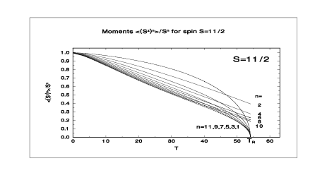
Figure 4: Results of a Green’s function calculation for the normalized moments $\langle(S^{z})^{n}\rangle/S^{n}$ for a monolayer and spin $S=11/2$ for $n=1,2,\ldots,11$. $T_{R}$ is the reorientation temperature.

In Figure 5 the equilibrium reorientation angles $\Theta_{0}$, and in Figure 6 the corresponding effective anisotropy coefficients $K_{2}(T)/K_{2}(0)$ are shown as functions of the temperature for spin quantum numbers ranging from $S=1$ to $S=6$, as calculated from the Green’s function method. The temperature dependence of both these quantites does not vary markedly with $S$. In the insets of the figures are the corresponding results for $\Theta_{0}$ and $K_{2}(T)/K_{2}(0)$ as obtained from a MFT for all interactions. As already seen for the magnetizations, a more pronounced spin dependence of $K_{2}(T)/K_{2}(0)$ is observed here also for MFT. Evidently, the spin quantum number $S$ has a larger influence on single-spin excitations (MFT) than on collective magnetic excitations (spin waves).

If scaled coupling constants are used, only a weak dependence of the spin quantum number $S$ on the magnetic quantities such as the magnetization, the reorientation angle, and the effective anisotropy is observed within the Green’s function method. Thus, one may perform calculations with a low spin, for which a considerably smaller system of equations has to be solved self-consistently. Results for higher spins can then be obtained by scaling. This is less justified within the MFT approximation.

We stress a result already obtained in reference FJK00 for spin $S=1$, namely that the effective anisotropies $K_{2}(T)$ as calculated within the RPA and within MFT have different temperature behaviours, particularly at low temperatures. In this temperature regime, the MFT exhibits an exponential behaviour, and RPA an almost linear behaviour of $K_{2}(T)$. Consequently, the use of MFT would lead to a considerably smaller value for $K_{2}(0)$ than that obtained with RPA, when the observed values of $K_{2}(T)$ (measured typically at $T/T_{C}\simeq 0.7$, e.g. exp ) are extrapolated to $T=0$. Note that only at $T=0$ are anisotropy coefficients available from ab-initio calculations, e.g. reference HB97 . These theoretical values can only be compared with experiment by extrapolating measurements at finite temperatures down to zero with the help of a theoretical model. Because of the drawbacks of MFT we propose performing this extrapolation with the results from the Green’s function method.

Figure 5: Equilibrium reorientation angle $\Theta_{0}$ as a function of the temperature for the systems of Figure 3 calculated with the Green’s function theory. The inset shows the corresponding results when applying MFT to all interactions.

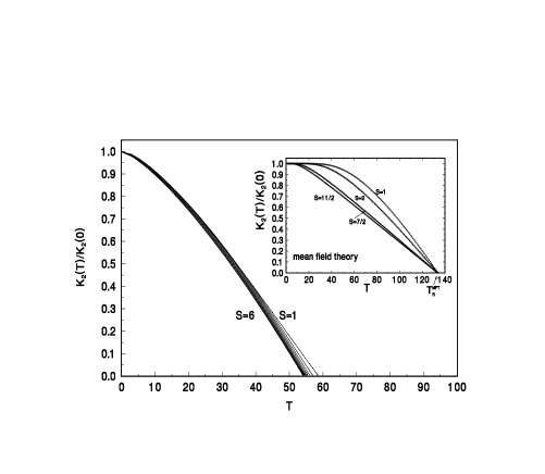
Figure 6: Effective anisotropy $K_{2}(T)/K_{2}(0)$ calculated with the Green’s function method as a function of the temperature for the systems of Figure 3. The inset shows the corresponding MFT results.

3.3 Ferromagnetic films with N layers

In this subsection we demonstrate that the formalism developed in Section 2 can be applied to the case of many layers. We study the magnetization, the reorientation angle, and the effective anisotropy as functions of the film thickness (characterized by the number of atomic layers, $N$). In all the examples shown in this subsection, the dipole coupling is included within the simplified mean field treatment as discussed above.

As examples we treat simple cubic films consisting of $N$ layers with spin $S=1$, using the same coupling parameters for all film layers (homogeneous film): $J=J_{ik}=100$, $K_{2,k}=K_{2}=1$, $g_{ik}=g=0.018$. These couplings are scaled as in Section 3.2 : $J\to J/S(S+1)$, $g\to g/S(S+1)$, $K_{2}\to K_{2}/S(S-1/2)$, and $B\to B/S$. All quantities are calculated for a small external magnetic field ${\bf B}=(0.1,0,0)$.

In Figure 7 we show the sublayer magnetizations $\langle S_{i}^{z}\rangle$, $i=1,\ldots,N$, as functions of the temperature for film thicknesses ranging between $N=1$ and $N=19$ layers. As expected, and also seen in MFT calculations JeB98 ; theo , for a homogeneous film, the magnetization of the surface layers is smaller than those of the interior layers because of the smaller coordination number for the surface. Also, the magnetizations of the $i$th and the $(N-i+1)$th layer are the same (twofold symmetry). For the parameters under consideration the reorientation temperature $T_{R}$ is close to the Curie temperature for perpendicular magnetization. Therefore, we see in Figure 7 that the value for the reorientation temperature $T_{R}$ (defined as the temperature where $\langle S^{z}_{i}\rangle=0$) exhibits a saturation behaviour as a function of the film thickness. Whereas there is a steep rise from $T_{R}(N=1)=58.55$ for the monolayer to $T_{R}(N=3)=103.08$ for the trilayer, there is only a small difference between $T_{R}(N=17)=135.11$ and $T_{R}(N=19)=135.67$.

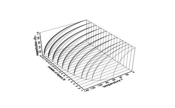
Figure 7: Sublayer magnetizations $\langle S^{z}_{i}\rangle$ as functions of the temperature for thin ferromagnetic films with $N$ layers and spin $S=1$. The reorientation temperatures $T_{R}^{N}$ for the different films can be read off from the curve in the $N-T$ plane, where $\langle S^{z}_{i}\rangle=0$. The same parameters are used for all layers: $B^{x}=0.1$, $J=100$, $K_{2}=1$, and $g=0.018$. They are scaled as described in the text.

Because in experiment only the average orientation of the thin film magnetization is measured one has to calculate this quantity from the model. In Figure 8 we show the average equilibrium reorientation angles $\Theta_{0}(N,T)$ of thin films with different thicknesses $N$ as functions of the temperature, where

$$\Theta_{0}(N,T)=\arctan\;\frac{\frac{1}{N}\sum_{i=1}^{N}\langle S_{i}^{x}\rangle}{\frac{1}{N}\sum_{i=1}^{N}\langle S_{i}^{z}\rangle}\;.$$ (48)

An alternative to calculating the average orientation angle is first to calculate the angles for each layer, $\Theta_{0,i}=\arctan(\langle S_{i}^{x}\rangle/\langle S_{i}^{z}\rangle)$, and then to average over the angles. The difference between both procedures turns out to be tiny.

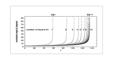
Figure 8: The average equilibrium reorientation angle $\Theta_{0}$ as a function of the temperature and film thickness. $N$ is the number of layers in each film and $T^{N}_{R}$ are the reorientation temperatures ($\Theta_{0}=90^{\circ}$).

In Figure 9 the average effective anisotropies $K_{2}(N,T)$ $/K_{2}(N,0)$ of thin films with different thicknesses $N$, calculated from equation (47), are shown as functions of the temperature. With increasing film thickness the action of the effective anisotropy extends to higher temperatures. In the inset we also show for $N=1$ and $N=19$ that the dependence of the anisotropies on the temperature is somewhat different for different layer thicknesses if one scales the temperature to the respective reorientation temperatures: $T/T_{R}(N)$. The curvature of the curve for the thick film ($N=19$) is more pronounced as that for the monolayer.

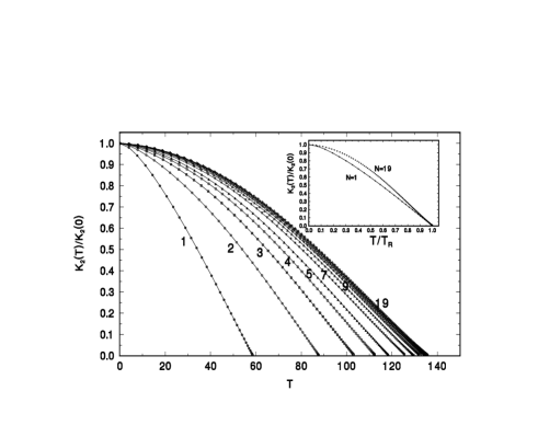
Figure 9: Average effective anisotropy $K_{2}(T)/K_{2}(0)$ as a function of the temperature and film thickness $N$. The inset demonstrates the different functional dependence of $K_{2}(T)/K_{2}(0)$ on the temperature for layers with $N=1$ and $N=19$ if the temperature $T$ is scaled with respect to the reorientation temperature $T_{R}$.

4 Discussion and conclusions

In the present paper we have extended the model of reference FJK00 in various respects and we have developed a succinct formulation of the final equations. This was made possible by utilizing the eigenvectors as well as the eigenvalues of the matrix governing the equations of motion for the set of Green’s functions, which has to be introduced when the calculation of several non-vanishing components of the magnetization is required. This new procedure, which for the monolayer and spin $S=1$ is fully equivalent to our earlier treatment FJK00 , provides a practicable way of extending the Green’s function spin wave theory to the reorientation of the magnetization of ferromagnetic films consisting of many layers and for general spin $S$.

We have applied the new method to the monolayer case with spins $S\geq 1$. We have found that the spin dependence of the magnetizations and the anisotropies as functions of the temperature is considerably less pronounced in RPA than in MFT if a proper scaling of the parameters of the model is applied . The corresponding curves saturate much more quickly in RPA than in MFT with increasing spin quantum number $S$. The temperature for complete reorientation $T_{R}$, on the other hand, does not change with $S$ in MFT, whereas there remains a slight spin dependence in RPA.

For the monolayer with spin $S=1$, we have investigated in detail the influence of the dipole coupling on the reorientation problem. Because, for realistic dipole coupling strengths, we found no big differences in treating the dipole coupling with its RPA or (non-dispersive) MFT approximations , cf. Appendix A, we chose to include the dipole coupling by means of the latter, which is relatively simple to handle and requires only a renormalization of the external magnetic field.

We emphasize that only by using our new method have we been able to treat the magnetic reorientation within a Green’s function approach for films with several layers. We have studied the field-induced magnetic reorientation and the effective anisotropy as functions of the film thickness and temperature for spin $S=1$ films. Investigations of films with $S\geq 1$ present no problem; they are only more time consuming.

In the present paper, we have only studied homogeneous films, but the method can also treat inhomogeneous films or multilayers by using layer-dependent coupling constants and magnetic moments. The magnetic reorientation could then be calculated for thin film or multilayer systems investigated experimentally. This will be pursued in forthcoming studies.

A few words concerning the applications of the present model are in order. A prerequisite is that the investigated systems can be modelled in a reasonable way by a local spin model of Heisenberg type. Moreover, it is required that higher order anisotropies are not important, a condition which is often not fulfilled.

Most results of the present paper are obtained for a small transverse field which initializes the reorientation. It is certainly of interest to calculate also phase diagrams in which the magnetic field is varied, and to compare with results obtained in reference Mil97 within a schematic model and in reference Us2000 on the basis of mean field theory.

The possibility of treating spins $S>1$ would also allow the treatment of the fourth-order uniaxial anisotropy $K_{4}$ as well as the quartic in-plane anisotropy. This, however, requires a proper decoupling procedure for the corresponding terms in the Green’s function theory which we do not have available at the moment. A phase diagram in the $K_{2}-K_{4}$ plane would then show the region of stable magnetization directions and would help in exploring the locations of temperature or film thickness driven magnetic reorientations. Also, one could determine whether the magnetic reorientation happens continuously or discontinuously.

Appendix A: The treatment of the dipole coupling

In this Appendix we show how the long-range magnetic dipole coupling can be considered within the RPA treatment of the magnetic reorientation. Furthermore, we show that a simplified treatment for interaction strengths small compared to the exchange interaction leads to a satisfactory description of the magnetic properties. For simplicity we consider only the case of a single layer ($N=1$).

As it should be, the magnetic dipole interaction leads to an additional dispersion in the magnon dispersion relation $\omega({\bf k})$. Applying the generalized Tyablikov (RPA) decoupling, equation (7), to the dipole interaction in the Green’s function equations of motion (5), $\langle\langle[S_{i}^{\alpha},{\cal H}^{\rm dipole}]_{-};$ $(S_{j}^{z})^{m}(S_{j}^{-})^{n}\rangle\rangle$, one obtains the following additional terms on the left side of equations (10)

$$\left(\begin{array}[]{ccc}-T_{\bf k}^{+}&-T_{\bf k}^{-}&-T_{\bf k}^{z}\\ (T_{\bf k}^{-})^{*}&T_{\bf k}^{+}&(T_{\bf k}^{z})^{*}\\ T_{\bf k}^{z\pm}&-(T_{\bf k}^{z\pm})^{*}&0\end{array}\right)\left(\begin{array}[]{c}G_{\eta}^{+,mn}\\ G_{\eta}^{-,mn}\\ G_{\eta}^{z,mn}\end{array}\right)\;.$$ (49)

Here a 2D Fourier transformation has been applied, and

$$T_{\bf k}^{+} = g\;\langle S^{z}\rangle\Big{(}T_{20}^{0}+T_{02}^{0}+\frac{1}{2}T_{20}^{\bf k}+\frac{1}{2}T_{02}^{\bf k}\Big{)}$$

$$T_{\bf k}^{-} = \frac{3}{2}\;g\;\langle S^{z}\rangle(T_{20}^{\bf k}-T_{02}^{\bf k}+2i\;T_{11}^{\bf k})$$ (50)

$$T_{\bf k}^{z} = g\;\langle S^{+}\rangle\Big{(}T_{20}^{\bf k}+T_{02}^{\bf k}+\frac{1}{2}T_{20}^{0}+\frac{1}{2}T_{02}^{0}\Big{)}$$

$$T_{\bf k}^{z\pm} = \frac{g}{4}\bigg{(}\langle S^{-}\rangle(T_{20}^{\bf k}+T_{02}^{\bf k}-T_{20}^{0}-T_{02}^{0})$$

$$-3\langle S^{+}\rangle(T_{20}^{\bf k}-T_{02}^{\bf k}-2i\;T_{11}^{\bf k})\bigg{)}\;,$$

where

$$T_{\mu\nu}^{\bf k}=\sum_{lm}\frac{(x_{l})^{\mu}(y_{m})^{\nu}}{(x_{l}^{2}+y_{m}^{2})^{5/2}}\;\exp(ik_{x}x_{l})\;\exp(ik_{y}y_{m})$$ (51)

are oscillating lattice sums, which can be evaluated with Ewald summation techniques as outlined for instance in reference jens97 .

As mentioned in the main body of the paper, the RPA treatment of the magnetic dipole coupling complicates the calculation of the magnetization considerably because of the presence of complex terms and dispersive (${\bf k}-$dependent) terms. Thus, as an approximation we neglect now the dispersive parts in the equations of motion (49) coming from the dipole coupling, and retain the non-dispersive terms only. This corresponds to a mean field treatment of the dipole coupling. Then equations (50) reduce to

$$T_{\bf k}^{+} = g\;\langle S^{z}\rangle(T_{20}^{0}+T_{02}^{0})$$

$$T_{\bf k}^{-} = 0$$ (52)

$$T_{\bf k}^{z} = \frac{g}{2}\;\langle S^{+}\rangle(T_{20}^{0}+T_{02}^{0})$$

$$T_{\bf k}^{z\pm} = -\frac{g}{4}\;\langle S^{-}\rangle(T_{20}^{0}+T_{02}^{0})\;.$$

This simplification allows the dipole coupling to be taken into account by a renormalization of the external magnetic field, and leads to equations (13) of Section 2.

By comparing to RPA, we shall show now that this approximation leads to satisfactory results for small dipole coupling strengths as found for instance in ferromagnetic $3d$- transition metal thin films. Because the general RPA treatment of the dipole coupling turns out to be fairly complicated, we consider only two limiting cases which are manageable, a perpendicular and an in-plane magnetization. An external magnetic field is not considered but can be easily added.

For spin $S=1$, one needs the Green’s functions $G_{ij}^{\pm,mn}$ $=\langle\langle S_{i}^{\pm};(S_{j}^{z})^{m}(S_{j}^{-})^{n}\rangle\rangle$ for $n=1$ and for $m=0$ and $m=1$. In case of the perpendicular magnetization, use of the RPA decoupling for the exchange interaction and the dipole coupling, and the Anderson-Callen decoupling for the single-ion anisotropy ($\Phi=\langle S^{z}\rangle\langle S^{z}S^{z}\rangle$ for $S=1$) leads to the following equations of motion (the $z$-axis is directed perpendicular to the plane)

$$\left(\begin{array}[]{cc}\omega-a&b\\ -b^{*}&\omega+a\end{array}\right)\left(\begin{array}[]{c}G^{+,m1}({\bf k},\omega)\\ G^{-,m1}({\bf k},\omega)\end{array}\right)=\left(\begin{array}[]{c}A^{+,m1}\\ A^{-,m1}\end{array}\right)\;,$$ (53)

with

$$a = \langle S^{z}\rangle\bigg{(}J\,(q-\gamma_{\bf k})-g\Big{(}T_{20}^{0}+T_{02}^{0}+\frac{1}{2}T_{20}^{\bf k}+\frac{1}{2}T_{02}^{\bf k}\Big{)}$$

$$-K_{2}\;\langle S^{z}S^{z}\rangle\bigg{)}$$

$$b = \frac{3}{2}\;g\;\langle S^{z}\rangle\Big{(}T_{20}^{\bf k}-T_{02}^{\bf k}+2i\,T_{11}^{\bf k}\Big{)}\;.$$ (54)

Solving these equations for the Green’s functions and applying the spectral theorem we obtain the following correlation functions

$$\langle(S^{z})^{m}S^{-}S^{+}\rangle = -\frac{1}{2}\,A_{-1}^{+,m1}$$

$$+\frac{1}{2\epsilon}\;\Big{(}a\,A_{-1}^{+,m1}-b\,A_{-1}^{-,m1}\Big{)}\coth\Big{(}\frac{\beta\epsilon}{2}\Big{)}\;,$$

$$\langle(S^{z})^{m}S^{-}S^{-}\rangle = \frac{1}{2}\,A_{-1}^{-,m1}$$ (55)

$$-\frac{1}{2\epsilon}\;\Big{(}a\,A_{-1}^{-,m1}-b^{*}\,A_{-1}^{+,m1}\Big{)}\coth\Big{(}\frac{\beta\epsilon}{2}\Big{)}\;,$$

where the dispersion relation is

$$\epsilon=\sqrt{a^{2}-|b|^{2}}\;\;.$$ (56)

Using now for $S=1$ the identities $S^{-}S^{+}=2-S^{z}-(S^{z})^{2}$ and $(S^{z})^{3}=S^{z}$, the inhomogeneities are given by

$$A_{-1}^{+,01}=2\langle S^{z}\rangle\;, A_{-1}^{+,11}=3\langle(S^{z})^{2}\rangle-\langle S^{z}\rangle-2\;,$$

$$A_{-1}^{-,01}=0\;,\hskip 28.45274pt A_{-1}^{-,11}=\langle S^{-}S^{-}\rangle\;.$$ (57)

For $m=0$ we obtain

$$\langle(S^{z})^{2}\rangle =2-\langle S^{z}\rangle(1+2\phi_{1})\;,\hskip 14.22636pt\langle S^{-}S^{-}\rangle=2\langle S^{z}\rangle\phi_{2}^{*}\;,$$

and for $m=1$

$$\langle S^{z}\rangle-\langle(S^{z})^{2}\rangle =(3\langle(S^{z})^{2}\rangle-\langle S^{z}\rangle-2)\phi_{1}-\langle S^{-}S^{-}\rangle\phi_{2}\;,$$

where sums (integrals) over the first Brillouin zone have to be performed for the quantities

$$\phi_{1} = \frac{1}{N}\sum_{\bf k}\Big{(}\frac{a}{2\epsilon}\,\coth\big{(}\frac{\beta\epsilon}{2}\big{)}-\frac{1}{2}\Big{)}\;,$$

$$\phi_{2} = \frac{1}{N}\sum_{\bf k}\frac{b}{2\epsilon}\,\coth\big{(}\frac{\beta\epsilon}{2}\big{)}\;.$$ (60)

From these equations we find the expectation values

$$\langle S^{z}\rangle = \frac{1+2\phi_{1}}{1+3\phi_{1}+3\phi_{1}^{2}+|\phi_{2}|^{2}}\;,$$ (61)

$$\langle(S^{z})^{2}\rangle = 2-\langle S^{z}\rangle(1+2\phi_{1})\;.$$ (62)

These equations are solved self-consistently for $\langle S^{z}\rangle$ and $\langle(S^{z})^{2}\rangle$.

In Figure 10 we show these expectation values with full RPA for the dipole coupling ($g=0.018$ estimated for Ni) for a monolayer using the parameters $J=100$, $K_{2}=1$, and for $g=0$ (no dipole coupling). For the perpendicular magnetization, the $\langle S^{-}S^{-}\rangle$ correlation is very small, and, within the line thickness of the curves, there is no difference between the full RPA and a RPA where one puts $\langle S^{-}S^{-}\rangle=0$ ($b=0$). Also shown are the corresponding results for the dipole coupling considered within the (non-dispersive) mean field treatment. In this case, not only $b=0$ but also the k-dependent terms in equation (54) connected with the dipole coupling are neglected, i.e.

$$a = \langle S^{z}\rangle\Big{(}J\,(q-\gamma_{\bf k})-g\,(T_{20}^{0}+T_{02}^{0})-K_{2}\,\langle S^{z}S^{z}\rangle\Big{)}\;,$$

$$b = 0\,.$$ (63)

As can be seen from Figure 10, the difference between a RPA and a MFT treatment of the dipole coupling is small.

Figure 10: Expectation value $\langle S^{z}\rangle$ for a monolayer with perpendicular magnetization and for spin $S=1$ as a function of the temperature. The dipole coupling ($g=0.018$ for Ni) is treated with full RPA, equation (54), and its mean field approximation, equation (63). For comparison we show also the result with vanishing dipole coupling ($g=0$). We have used $J=100$, $K_{2}=1$, and a vanishing external field ${\bf B}=0$.

Figure 11: In-plane magnetization $\langle S^{x}\rangle$ for a monolayer with spin $S=1$ as function of the temperature. The dipole coupling ($g=0.018$) is treated with full RPA, equation (64), with RPA putting $\langle S^{-}S^{-}\rangle=0$, i.e. $b=0$ in equation (LABEL:B9), and with MFT, equation (65). The $\langle S^{-}S^{-}\rangle_{RPA}$ correlation is also shown.

The situation is somewhat different for an in-plane magnetization. In this case the single-ion anisotropy is not active ($\Phi=0$), and the dipole term is, in accordance with the Mermin-Wagner theorem, the only term which induces a finite magnetization. In an RPA treatment of the dipole coupling the magnetization in the plane is not isotropic and one has to introduce an in-plane angle with respect to a main axis of the square lattice. By putting this angle equal to zero one obtains for the quantities $a$ and $b$, cf. equation (53),

$$a = \langle S^{z}\rangle\Big{(}J\,(q-\gamma_{\bf k})+\frac{g}{2}\,\big{(}T_{20}^{0}+T_{02}^{0}-T_{02}^{\bf k}+2\,T_{20}^{\bf k}\big{)}\Big{)}\;,$$

$$b = \frac{3}{2}\;g\;\langle S^{z}\rangle\;T_{02}^{\bf k}\;.$$ (64)

Using the mean field approximation for the dipole coupling by neglecting the corresponding k-dependent terms one obtains for the in-plane magnetization

$$a = \langle S^{z}\rangle\Big{(}J\,(q-\gamma_{\bf k})+\frac{g}{2}\,\big{(}T_{20}^{0}+T_{02}^{0}\big{)}\Big{)}\;,$$

$$b = 0\;.$$ (65)

Within the formalism above, the quantization $z$-axis is now directed in-plane, which corresponds to the $x$-direction of our original reorientation problem. The corresponding results are shown in Figure 11. Here the difference between the full RPA and MFT is somewhat larger, because the expectation value $\langle S^{-}S^{-}\rangle$ is not as small as in the case for the perpendicular magnetization. In particular the Curie temperature is appreciably lower than in MFT. This, however, is the most extreme case, and is an upper limit for the error one makes if the dipole coupling is treated by MFT for the reorientation problem. As also shown in Figure 11 the MFT result is close to the RPA result only when the $\langle S^{-}S^{-}\rangle$ correlation is neglected.

In summary, the error is small for the perpendicular orientation and will increase with increasing polar angle, but is expected to stay below the error for the in-plane case when replacing the full RPA treatment of the dipole coupling by the simplified, non-dispersive MFT. With this discussion in mind we use for the reorientation problem of the present paper the mean field approximation for the dipole coupling. We do so also because its full RPA treatment is quite complicated and time-consuming. If the ratio between the dipole coupling strength and the exchange coupling becomes larger, as expected e.g. for rare earth ferromagnets, the error will increase and the simplified treatment is less justified. In this case one is faced with the more complicated full RPA treatment of the dipole coupling.

Finally, we mention that the magnetic dipole coupling can be taken into account also via its mean field approximation when calculating the magnetic reorientation with the Schwinger-Boson theory Timm00 . However, the proper inclusion of the long-range character of this interaction, which leads to additional momentum-dependent terms in the magnon dispersion relation, is practically impossible within this method.

Appendix B: Treating ${\bf S\geq 1}$

In this Appendix we show how the regularity conditions, which have been calculated in FJK00 for $S=1$, can be deduced for general spin quantum numbers $S$. The regularity condition (33) for $m=0,n=1$ yields

$$\frac{H^{\pm}}{\tilde{H}^{z}}=\frac{B^{\pm}}{Z}\;,$$ (66)

and can therefore be written for general $m,n$ in the form

$$-2\,Z\,A_{-1}^{z,mn}=A_{-1}^{+,mn}\,B^{-}+A_{-1}^{-,mn}\,B^{+}\;.$$ (67)

The $z$-component of equation (38), from which the correlations have to be calculated, reads then explicitly

$$2\,\frac{B^{+}B^{-}}{Z^{2}}\,\Big{\langle}(S^{z})^{m}(S^{-})^{n}S^{z}\Big{\rangle}-\frac{B^{-}}{Z}\,\Big{\langle}(S^{z})^{m}(S^{-})^{n}S^{+}\Big{\rangle}$$

$$\hskip 56.9055pt-\frac{B^{+}}{Z}\,\Big{\langle}(S^{z})^{m}(S^{-})^{n}S^{-}\Big{\rangle}$$

$$= \frac{1}{2}\,A_{-1}^{+,mn}\,\frac{E_{\bf k}}{\tilde{H^{z}}}\,\frac{B^{-}}{Z}\,\Big{[}\frac{E_{\bf k}}{\tilde{H^{z}}}-\coth\big{(}\frac{\beta E_{\bf k}}{2}\big{)}\Big{]}$$

$$\hskip 56.9055pt+\frac{1}{2}\,A_{-1}^{-,mn}\,\frac{E_{\bf k}}{\tilde{H^{z}}}\,\frac{B^{+}}{Z}\,\Big{[}\frac{E_{\bf k}}{\tilde{H^{z}}}+\coth\big{(}\frac{\beta E_{\bf k}}{2}\big{)}\Big{]}\,.$$

We express all correlation functions occuring in this equation in a standard form where all powers of $S^{z}$ are written to the left of the powers of $S^{-}$:

$$C(m,n)=\langle(S^{z})^{m}(S^{-})^{n}\rangle\,.$$ (69)

Then, with the relations $[S^{z},(S^{-})^{n}]_{-}=-n\,(S^{-})^{n}$ and $S^{-}S^{+}=S(S+1)-S^{z}-(S^{z})^{2}$, we find that

$$\langle(S^{z})^{m}(S^{-})^{n}S^{z}\rangle = n\,C(m,n)+C(m+1,n)\ ,$$

$$\langle(S^{z})^{m}(S^{-})^{n}S^{+}\rangle = \big{(}S(S+1)-n\,(n-1)\big{)}\,C(m,n-1)$$

$$-(2n-1)\,C(m+1,n-1)-C(m+2,n-1)\ ,$$

$$\langle(S^{z})^{m}(S^{-})^{n}S^{-}\rangle = C(m,n+1)\;.$$ (70)

The commutators can also be expressed in terms of the $C(m,n)$ using the binomial series

$$A_{-1}^{z,mn} = -nC(m,n)\ ,$$

$$A_{-1}^{+,mn} = \Big{\langle}\Big{[}\big{(}(S^{z}-1)^{m}-(S^{z})^{m}\big{)}S^{-}S^{+}+2\,S^{z}\,(S^{z}-1)^{m}$$

$$+(n-1)\,(n+2S^{z})(S^{z})^{m}\Big{]}(S^{-})^{n-1}\Big{\rangle}$$

$$= S(S+1)\sum_{i=1}^{m}\left(\begin{array}[]{c}m\\ i\end{array}\right)(-1)^{i}\,C(m-i,n-1)$$

$$+\sum_{i=2}^{m+1}\left(\begin{array}[]{c}m+1\\ i\end{array}\right)(-1)^{i+1}\,C(m+2-i,n-1)$$

$$+(2n+m)\,C(m+1,n-1)+n(n-1)C(m,n-1)\;,$$

$$A_{-1}^{-,mn} = \Big{\langle}\big{[}(S^{z}+1)^{m}-(S^{z})^{m}\big{]}(S^{-})^{n+1}\Big{\rangle}$$ (79)

$$= \sum_{i=1}^{m}\left(\begin{array}[]{c}m\\ i\end{array}\right)C(m-i,n+1)\;.$$

Now by putting equation (79) into equation (67) the regularity conditions for all $m$ and $n$ can be written in terms of correlations defined in the standard form:

$$2\,Z\,n\,C(m,n)=$$

$$B^{-}\Big{[}S(S+1)\,\sum_{i=1}^{m}\left(\begin{array}[]{c}m\\ i\end{array}\right)(-1)^{i}\,C(m-i,n-1)$$ (82)

$$+\sum_{i=2}^{m+1}\left(\begin{array}[]{c}m+1\\ i\end{array}\right)(-1)^{i+1}\,C(m+2-i,n-1)$$ (85)

$$+(2n+m)\,C(m+1,n-1)+n\,(n-1)\,C(m,n-1)\Big{]}$$

$$+B^{+}\,\sum_{i=1}^{m}\left(\begin{array}[]{c}m\\ i\end{array}\right)\,C(m-i,n+1)\;.$$ (88)

For a given spin $S$, this set of linear equations for the correlations has to be solved for all $m+n\leq 2S+1$. The solutions have to be put via equations (70) together with (79) into equations (Appendix B: Treating ${\bf S\geq 1}$), thus leading to a set of $2S$ equations for the moments $\langle(S^{z})^{p}\rangle$ ($p=1,\ldots,2S$), which have to be solved self-consistently. The highest moment $\langle(S^{z})^{2S+1}\rangle$ has been eliminated in favour of the lower ones through the relation $\prod_{M_{S}}(S^{z}-M_{S})=0$.

References

- (1) A. Ecker, P. Fröbrich, P.J. Jensen, P.J. Kuntz, J. Phys.: Condens. Matter 11, 1557 (1999).
- (2) P. Fröbrich, P.J. Jensen, P.J. Kuntz, Eur. Phys. J. B 13, 477 (2000).
- (3) A. Moschel, K.D. Usadel, Phys. Rev. B 49, 12868 (1994); P.J. Jensen, K.H. Bennemann, in ‘Magnetism and Electronic Correlations in Local-Moment Systems: Rare-Earth Elements and Compounds’, ed. M. Donath, P.A. Dowben and W. Nolting, (World Scientific, Singapore, 1998), p. 113-141.
- (4) P.J. Jensen, K.H. Bennemann, Solid State Comm. 100, 585 (1996); ibid. 105, 577 (1998); A. Hucht, K.D. Usadel, Phys. Rev. B 55, 12309 (1997).
- (5) P.J. Jensen, K.H. Bennemann, P. Poulopoulos, M. Farle, F. Wilhelm, K.Baberschke, Phys. Rev. B 60, R14884 (1999).
- (6) R. Schiller, W. Nolting, Solid State Commun. 110, 121 (1999).
- (7) P. Bruno, Phys. Rev. B 43, 6015 (1991).
- (8) L.P. Shi, W.G. Wang, J. Phys.: Condens. Matter 4, 7997 (1992).
- (9) R.P. Erickson, D.L. Mills, Phys. Rev. B 44, 11825 (1991).
- (10) C. Timm, P.J. Jensen, Phys. Rev. B 62, 5634 (2000).
- (11) S.V. Tyablikov, Ukr. Mat. Zh.11, 287 (1959).
- (12) F.B. Anderson, H.B. Callen, Phys. Rev. 136, A1068 (1964).
- (13) M.E. Lines, Phys. Rev. 156, 534 (1967).
- (14) S.V. Tyablikov, Methods in the quantum theory of magnetism (Plenum Press, New York, 1967); K. Elk and W. Gasser, Die Methode der Greenschen Funktionen in der Festkörperphysik (Akademie-Verlag, Berlin, 1978); W. Nolting, Quantentheorie des Magnetismus, vol.2 (B.G. Teubner, Stuttgart, 1986).
- (15) L.D. Landau, E.M. Lifschitz, vol. VIII, (Akademie-Verlag, Berlin, 1974).
- (16) S.V. Vonsovskii, ‘Magnetism’, vol. 2, chapt. 23 (J. Wiley Sons, 1974).
- (17) P.J. Jensen, Ann. Physik 6, 317 (1997).
- (18) G. Lugert, W. Robl, L. Pfau, M. Brockmann, G. Bayreuther, J. Magn. Magn. Mater. 121, 498 (1993); O. Schulte, F. Klose, W. Felsch, Phys. Rev. B 52 6480 (1995); G. Garreau, E. Beaurepaire, K. Ounadjela, M. Farle, Phys. Rev. B 53, 1083 (1996); M. Farle, B. Mirwald-Schulz, A. N. Anisimov, W. Platow, K. Baberschke, Phys. Rev. B 55, 3708 (1997), and references therein.
- (19) O. Hjortstam, K. Baberschke, J.M. Wills, B. Johansson, O. Erickson, Phys. Rev. 55, 15026 (1997); C. Uiberacker, J. Zabloudil, P. Weinberger, L. Szunyogh, C. Sommers, Phys. Rev. Lett. 82, 1289 (1999), and references therein.
- (20) Y.T. Millev, H.P. Oepen, J. Kirschner, Phys. Rev. B 57, 5837 and 5848 (1998).
- (21) A. Hucht, K.D. Usadel, Phil. Mag. B 80, 275 (2000).