Swelling kinetics of the onion phase

Abstract

A theory is presented for the behavior of an array of multi-lamellar vesicles (the onion phase) upon addition of solvent. A unique feature of this system is the possibility to sustain pressure gradients by tension in the lamellae. Tension enables the onions to remain stable beyond the unbinding point of a flat lamellar stack. The model accounts for various concentration profiles and interfaces developing in the onion as it swells. In particular, densely packed ‘onion cores’ are shown to appear, as observed in experiments. The formation of interfaces and onion cores may represent an unusual example of stabilization of curved interfaces in confined geometry.

1 Introduction

The self-assembly of amphiphilic molecules (surfactants) in solution has been the subject of intensive research in the past decades Benshaul ; GompperSchick . Such molecules may self-assemble into a wide variety of aggregate morphologies such as micelles, bilayers, bilayer stacks (the lamellar, or L_α phase) and various other liquid-crystalline structures. The richness of these phenomena is both useful for numerous chemical and biochemical applications and challenging for basic research.

Yet another morphology of amphiphilic self-assembly has recently drawn considerable attention. When a lamellar (L_α) phase is subjected to shear, it undergoes a dynamic transition into an array of close-packed multilayer vesicles, referred to as the onion phase Roux1 ; Roux2 ; Roux3 ; Roux4 ; Roux5 . The typical size of an ‘onion’ is of order 1–10 $\mu$m, whereas the inter-membrane spacing is of order 10 nm, and the thickness of the membrane itself is of order of a few nm. Thus, each onion comprises a spherical stack of more than several hundred spaciously packed membranes. Although this structure is not an equilibrium one, it may remain stable for days. In addition, one can control the size of the onions by changing the shear rate Roux1 , and encapsulate small particles inside them encapsulation . These appealing features have potential applications, e.g., in the pharmaceutical industry.

Various properties of the onion phase are not well understood theoretically. In particular, the detailed mechanism of the L_α-to-onion dynamic transition has not yet been established ZilmanGranek . Simple scaling arguments have been successful in accounting for the dependence of the onion size on shear rate and inter-membrane spacing Roux2 ; Lekker , as well as the viscoelastic behavior of the onion phase Panizza .

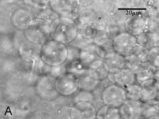
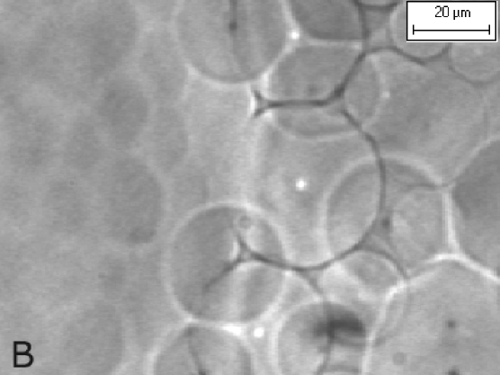
Figure 1: Formation of ‘onion cores’ upon dilution. (A) SDS–octanol–brine system Buchanan2 . (B) AOT–brine system Buchanan1 . (Pictures courtesy of M. Buchanan.)

In the current work we focus on another property of the onion phase — its behavior under dilution. This aspect has been investigated in recent experiments Buchanan1 ; Buchanan2 . When a regular L_α phase is diluted, the added solvent is accommodated in the inter-membrane spacings. The membrane stack thereby swells, until a ‘melting’ transition into a disordered L₃ (‘sponge’) phase occurs GompperSchick ; Safran . The onion phase is observed to dissolve into L₃ as well. Yet, because of the confined spherical geometry, the stack cannot swell without a supply of additional surfactant. (Amphiphilic membranes, to a good approximation, are practically inextensible inextensible .) As a result, the dissolution progresses very slowly (over days) through onion coalescence and disintegration, giving rise at intermediate times to various defects and instabilities. In particular, the formation of dense onion cores has been observed in two different systems Buchanan1 ; Buchanan2 , as is demonstrated in Fig. 1.

Our model of onion swelling relies on an assumption concerning separation of time scales. The time scale of swelling of the entire onion is assumed to be much longer than the one required for internal equilibration within the onion. Experimentally, the former is of order of a few hours. The latter is related to the time scale characterizing the formation of passages (‘necks’) between adjacent membranes passages . We thus assume that passages form on time scales much shorter than hours. Though reasonable, the validity of this assumption is still to be established experimentally. There is a third time scale, corresponding to onion coalescence and disintegration into L₃. Experimentally, it is found to be of order of days and will be ignored here. Thus, although the onion phase is a system far from equilibrium, the above assumption allows us to present an essentially equilibrium model of onion swelling.

A fundamental question arising from the study of onion dissolution concerns the possibility to stabilize a curved interface between two coexisting domains in confined geometry. In common situations such a possibility does not exist. (For example, a liquid droplet inside a coexisting vapor phase is unstable, and will either shrink and vanish or expand to a macroscopic phase Kittel ; this is the origin of nucleation barriers in 1st-order phase transitions.) Stable interfaces in confined geometry are found in specific systems, such as magnetic garnet films, block-copolymer melts, phospholipid monolayers and microemulsions, exhibiting modulated phases Andelman95 . Competing interactions in such systems lead to a negative surface tension (i.e., negative stiffness term in a coarse-grained Ginzburg-Landau free energy), which is stabilized by higher-order terms. This gives rise to a finite characteristic length scale of interface modulation Andelman95 . As seen in Fig. 1, onions under dilution seem to exhibit a stable interface between a confined, dense core and a dilute shell. We shall try to demonstrate that this behavior might represent a new way to stabilize a curved interface, arising from the unique ability of onions to sustain pressure gradients at equilibrium.

In section 2 we extend a simple theory for the unbinding transition in a flat L_α phase Milner92 to the case of membranes with tension. Based on this extension, we formulate in section 3 a model of a single onion as an inhomogeneous, spherical membrane stack. We then present the resulting concentration and tension profiles in the onion. Finally, in section 4, we summarize the results and point at future directions.

2 Lamellar Phase with Tension

Fluid membranes in a lamellar stack experience steric repulsion arising from their reduced undulation entropy (the Helfrich interaction) Helfrich1 . In the case of tensionless membranes the interaction energy per unit area is

$$f_{\rm und}(D)=\frac{bT^{2}}{\kappa D^{2}},$$ (1)

where $T$ is the temperature (in energy units, i.e., $k_{\rm B}\equiv 1$), $\kappa$ the bending rigidity of the membranes, and $D$ the inter-membrane spacing. (The numerical prefactor $b$ is still under controversy Sornette ; Helfrich’s calculation Helfrich1 gives $b=3\pi^{2}/128\simeq 0.2$, whereas computer simulations Lipowsky89 yield a lower value of $b\simeq 0.06$.) The long range of the Helfrich interaction, Eq. (1), results from the ‘floppiness’, i.e., strong thermal undulations, of tensionless membranes. The interplay between the Helfrich repulsion and other, direct interactions determines when a lamellar stack of membranes becomes unstable and unbinds. The rich critical behavior exhibited by this system was thoroughly investigated using functional renormalization group techniques Nelson_Leibler ; LipowskyLeibler .

Subsequently, a much simpler theory for the unbinding of a lamellar membrane stack was proposed Milner92 . It employs a similar argument to Flory’s for polymers — since the stack is a ‘soft’, entropy-dominated system, one has to accurately account for entropy [i.e., the Helfrich repulsion, Eq. (1)], while the other interactions can be incorporated in an approximate, 2nd-virial term. The resulting (grand-canonical) free energy per unit volume of the lamellar stack is

$$f(\phi)=\frac{1}{2}\phi^{3}-\chi\phi^{2}-\mu\phi,$$ (2)

where $\phi\equiv\delta/D$ is the surfactant volume fraction ($\delta$ being the membrane thickness), $\chi$ is a 2nd-virial coefficient, and $\mu$ the surfactant chemical potential. All energy densities have been scaled by $2bT^{2}/(\kappa\delta^{3})$. For $\chi>0$ the free energy (2) describes a 1st-order unbinding transition as $\mu$ is lowered. The chemical potentials and volume fractions corresponding to the binodal and spinodal of this transition are

$$\mu_{\rm bin} = -\chi^{2}/2,\ \ \ \ \phi_{\rm bin}=\chi$$

$$\mu_{\rm sp} = -2\chi^{2}/3,\ \ \ \phi_{\rm sp}=2\chi/3.$$ (3)

The free energy (2) also has a critical point at $\mu=\chi=0$, which is of much theoretical interest Nelson_Leibler , but of no relevance to the current discussion; hereafter, a positive value of $\chi$ is assumed.

Consider now a stack of membranes having tension $\sigma$. Surface tension strongly suppresses membrane undulations and, hence, the fluctuation-induced interaction between tense membranes has a much shorter range. The calculation of this interaction is more complicated than for tensionless membranes Sornette . Renormalization-group calculations RG_tension and computer simulations Netz95 yield an exponential decay with distance. A simpler, self-consistent calculation of this interaction Seifert gives

$$f_{\rm und}(D)=\frac{bT^{2}}{\kappa D^{2}}\left[\frac{D/l_{T}}{\sinh(D/l_{T})}\right]^{2},$$ (4)

where $l_{T}$ is the length arising from the combination of tension and thermal energy, $l_{T}\equiv(2T/\pi\sigma)^{1/2}$. The dimensionless parameter $x\equiv D/l_{T}=\delta/(l_{T}\phi)$, depending on both $\sigma$ and $\phi$, determines whether the tension has a significant effect on the interaction. For $x\ll 1$ $f_{\rm und}$ coincides with the tensionless expression, Eq. (1), whereas for $x\gg 1$ the tension strongly suppresses membrane undulations and the interaction decays exponentially with distance, in accord with the renormalization-group result RG_tension . (The numerical prefactor in $l_{T}$ was chosen so as to recover the renormalization-group result for high tension.) For brevity we use hereafter the following notation:

$$G(x) \equiv -\frac{1}{2\sinh^{2}x},\ \ \ g(x)\equiv\frac{{\rm d}G}{{\rm d}x}=\frac{\cosh x}{\sinh^{3}x},$$

$$g^{\prime}(x) \equiv \frac{{\rm d}g}{{\rm d}x}=\frac{4\sinh^{2}x-3}{\sinh^{4}x}.$$

The ‘Flory-like’ free energy per unit volume in the tense case is

$$f(\phi,\sigma)=-x^{2}G(x)\phi^{3}-\chi\phi^{2}-\mu\phi,$$ (5)

where the energy densities have been scaled, again, by $2bT^{2}/(\kappa\delta^{3})$. (Note that $x$ should not be taken as an independent degree of freedom but as $\phi$-dependent. The two independent degrees of freedom are $\phi$ and $\sigma$. Nevertheless, $x$ is extensively used below, in order to make the formulation more concise.)

Due to the additional degree of freedom — membrane tension — bound stacks can be stabilized even beyond the unbinding point of the tensionless case, i.e., for $\mu<\mu_{\rm sp}$. Hence, instead of a transition point there is a transition line, $\sigma^{*}(\mu)$, such that the stack is bound for $\sigma>\sigma^{*}$, and unbound for $\sigma<\sigma^{*}$. The equations for the binodal and spinodal lines are:

binodal: $$2\frac{G(x)+xg(x)}{[x^{2}g(x)]^{2}}=\frac{\mu}{\mu_{\rm bin}},\ \ \ \ \phi=\frac{\chi}{x^{3}g(x)}$$ (6)

spinodal: $$6\frac{G(x)-xg(x)-x^{2}g^{\prime}(x)}{[x^{3}g^{\prime}(x)]^{2}}=\frac{\mu}{\mu_{\rm sp}},$$

$$\phi=-\frac{2\chi}{x^{4}g^{\prime}(x)}.$$

The two lines are drawn in Fig. 2A. Figure 2B shows the line $x^{*}(\mu)$ corresponding to the binodal. When $\mu$ is slightly lower than $\mu_{\rm bin}$, the value of $x^{*}$ required to stabilize the stack increases sharply. On the other hand, values of $x^{*}$ much larger than 1 are required only for chemical potentials much lower than $\mu_{\rm bin}$. Hence, realistic values for $x^{*}$ should be of order 0.1–3.

3 Onion Swelling

3.1 The Model

In view of the assumption regarding separation of time scales, presented in section 1, we consider the onion as a spherical stack of constrained size. (Recall that the initial size of an onion is, by itself, determined not by thermodynamic equilibrium but by the shear rate that led to its formation Roux1 .) As dilution progresses, the constrained radius, $R$, increases slowly, such that at any instant the interior of the onion can be assumed in thermodynamic equilibrium. This implies, in particular, that the entire onion has a single, uniform chemical potential, $\mu$. Since the temperature, $T$, and the total number of surfactant molecules in the onion, $N$, are taken as fixed, $\mu$ must continuously decrease upon swelling. Thus, the equilibrium ensemble relevant to the actual dilution process (at time scales shorter than hours) is that of fixed $(T,R,N)$, where $R$ is regarded as a slowly increasing external parameter, leading to a slow decrease in $\mu$ and $p_{0}$, the osmotic pressure. For mathematical convenience, the model is formulated in the equivalent ensemble of fixed $(T,p_{0},\mu)$, where $\mu$ is is a slowly decreasing parameter.

As mentioned in section 1, each onion comprises a stack of many spaciously packed membranes. It is therefore justified to employ a coarse-grained, continuum model. Unlike a flat lamellar phase, the inter-membrane spacing in the onion is not expected to be uniform. Hence, we allow for non-uniform profiles, writing a Ginzburg-Landau free energy of the form

$$F[\phi(\vec{r}),\sigma(\vec{r})]=\int{\rm d}\vec{r}\left[\frac{1}{2}\Omega|\nabla\phi|^{2}+f(\phi,\sigma)\right]+\frac{4\pi}{3}p_{0}R^{3}.$$ (7)

The free energy density, $f(\phi,\sigma)$, has been defined in equation (5), and the integration is over the volume of the onion. An energetic penalty for concentration gradients has been included in equation (7), where $\Omega$ is a stiffness coefficient. The Lagrange multiplier $p_{0}$ should ensure that the onion radius has the constrained value $R$.

The state of the onion is defined by the concentration profile $\phi(r)$ (or, equivalently, by the set of inter-membrane spacings). The equilibrium concentration profile is thereby found from a variation principle. A major theoretical complication is the fact that the tension in the membranes enters at two distinct levels—as a macroscopic parameter, e.g., balancing the pressure difference across a membrane, and as a microscopic parameter having a dramatic effect on membrane interaction. In order to overcome this obstacle we use a self-consistent scheme. We assume that the membranes have attained certain values of tension, leading to a (still unknown) profile $x(r)$. Subsequently, we find the resulting concentration and pressure profiles and then require self-consistency, i.e., that the presumed tension in the membranes balance the pressure gradients. Note that this self-consistency does not require that the tension profile be smooth. Hence, no penalty for spatial changes in tension has been included in equation (7); near-by membranes may have very different tensions. In practice, the formation of passages should act to equalize the tension between layers and, hence, a certain penalty for tension differences is expected. We assume that such a tension-gradient term would not have a drastic effect on the results. Hence, we omit it to avoid addition of another parameter to the model.

3.2 Profile Equations

By taking the variation of $F$ with respect to $\phi(r<R)$ we obtain the first profile equation,

$$\Omega\nabla^{2}\phi+x^{2}[G(x)-xg(x)]\phi^{2}+2\chi\phi+\mu=0,$$ (8)

where, for our spherical-symmetric case, $\nabla^{2}={\rm d}^{2}/{\rm d}r^{2}+(2/r){\rm d}/{\rm d}r$. (Recall that the variation is taken while keeping $\sigma$, not $x$, fixed.)

Equation (8), obtained from a variation of a Ginzburg-Landau functional, is of the generic form widely used to study interfaces Langer . It is equivalent to imposing a uniform chemical potential throughout the system. Such a profile equation is usually supplemented by boundary conditions for the order parameter and its gradient far away from the interface, that ensure the uniformity of pressure. Such a system of equations is over-determined (a 2nd-order equation with four boundary conditions). It has a solution for a flat geometry, but does not have one for a confined (e.g., spherical) geometry. Thus, such a Ginzburg-Landau formalism cannot in general produce stable, confined interfaces. However, the onion phase has a very special property. Since the system is composed of concentric closed sheets, the pressure need not be uniform throughout the system; pressure gradients can be sustained by the tension in the membranes. In particular, if the system is divided into coexisting domains, the pressure does not have to be equal in the different domains. This property bypasses the usual uniform-pressure boundary conditions. They are to be replaced by an equation, derived below, balancing pressure gradients and tension.

Using Green’s identity and equation (8), we can rewrite the free energy at equilibrium as

$$F = -\int{\rm d}\vec{r}\frac{1}{2}\phi\{x^{2}[G(x)+xg(x)]\phi^{2}+\mu\}$$ (9)

$$+4\pi R^{2}\frac{1}{2}\Omega\phi(R)\frac{{\rm d}\phi(R)}{{\rm d}r}+\frac{4\pi}{3}R^{3}p_{0},$$

and identify the integrand as the local pressure,

$$p=\frac{1}{2}\phi\{x^{2}[G(x)+xg(x)]\phi^{2}+\mu\}.$$ (10)

Local balance between the pressure gradient and membrane tension is accounted for by a Laplace equation,

$$\hat{\sigma}_{i}=\frac{1}{2}r_{i}(p_{i-1}-p_{i})\simeq-\frac{1}{2}rD(r)\frac{{\rm d}p}{{\rm d}r},$$ (11)

where $\hat{\sigma}_{i}$ is the rescaled tension (having dimension of length) of membrane $i$, $r_{i}$ its radius, and $p_{i}$ the pressure just outside it. In the second equality we have assumed that the pressure profile is a smooth function on the length scale of $D$, the inter-membrane spacing. Equation (11) ensures that the pressure gradients resulting from the concentration profile are consistent with the presumed tension profile. For the sake of mathematical convenience, we shall treat the tension profile as a smooth function as well, i.e., represent spatial variations of $\sigma$ by a first derivative, ${\rm d}\sigma/{\rm d}r$. Since the model allows for sharp changes in $\sigma$, this approximation is merely technical and not physically corroborated. Consequently, the sharp changes will show up as singularities in an otherwise smooth tension profile, and will have to be treated separately to ensure that the smoothness of $\phi$ and $p$ is maintained. When equation (10) is substituted in equation (11), the smoothness assumption leads to the following, second profile equation:

$$[2G(x)+4xg(x)+x^{2}g^{\prime}(x)]\frac{1}{x}\frac{{\rm d}x}{{\rm d}r}$$

$$+\{3[G(x)+xg(x)]+\frac{\mu}{x^{2}\phi^{2}}\}\frac{1}{\phi}\frac{{\rm d}\phi}{{\rm d}r}+\frac{4\varepsilon}{r}=0,$$ (12)

where $\varepsilon\equiv\kappa/(\pi bT)$.

The profile equations (8) and (12), along with appropriate boundary conditions, determine the profiles $\phi(r)$ and $x(r)$.

3.3 Boundary Conditions

The onion is in contact with the surrounding environment through its outer layer. This layer requires a separate treatment, so as to yield the boundary conditions for the profile equations (8) and (12), i.e., $\phi(R)$, $x(R)$ and ${\rm d}\phi(R)/{\rm d}r$. We employ a self-consistent scheme similar to the one of section 3.2, i.e., using a variation principle for $\phi(R)$ and requiring that $\sigma(R)$ balance the pressure difference across the outer membrane.

Discretization of the integral in equation (7) and taking the variation of $F$ with respect to $\phi(R)$ give the boundary condition for the concentration gradient,

$$\frac{{\rm d}\phi(R)}{{\rm d}r}=-\left.\frac{\delta}{\Omega}\{x^{2}[G(x)-xg(x)]\phi^{2}+2\chi\phi+\mu\}\right|_{r=R}.$$ (13)

Variation of $F$ [Eq. (9)] with respect to $R$ yields the mechanical equilibrium (Laplace) equation for the outer membrane,

$$\frac{1}{2}\Omega\phi(R)\frac{{\rm d}\phi(R)}{{\rm d}r}=\frac{1}{2}R\{p[\phi(R),\sigma(R)]-p_{0}\},$$ (14)

where $p[\phi(R),\sigma(R)]$ is the pressure just inside the outer sheet, whose dependence on $\phi(R)$ and $\sigma(R)$ is given by equation (10). The multiplier $p_{0}$, coupled to the total volume [see equation (7)], is the external osmotic pressure exerted on the onion, i.e., the pressure just outside the outer sheet. Hence, the left-hand side of equation (14) is identified as the tension of the outer layer, $\hat{\sigma}(R)$. This observation, together with equation (13) and the definition of $x$, $\hat{\sigma}=\varepsilon\delta x^{2}\phi^{2}$, lead to two equations for $x(R)$ and $\phi(R)$,

$$x^{2}[G(x)-xg(x)]\phi^{2}+2(\chi+\varepsilon x^{2})\phi+\mu=0$$ (15)

$$x^{2}[G(x)+xg(x)]\phi^{2}-\frac{4\varepsilon\delta}{R}x^{2}\phi+\mu-\frac{2p_{0}}{\phi}=0.$$ (16)

One can proceed using boundary conditions (15) and (16). Yet, the formulation can be further simplified by employing an additional assumption. Prior to dilution, the onion is in contact with the outer membranes of neighboring onions in the close-packed phase. This situation persists as long as the unbinding point of the regular L_α phase has not been reached. During this initial stage of dilution the inter-membrane spacing inside the onion is equal to the spacing between the outer membranes of neighboring onions (i.e., $\phi$ is uniform throughout the sample). Consequently, the pressure is equal on both sides of the outer membrane and its tension vanishes, $x(R)=0$. The profile equations (8) and (12) then have the trivial uniform solution $x(r)\equiv 0,\phi(r)\equiv\phi(R)$. When the unbinding point is reached, $\mu<\mu_{\rm bin}$, the onion becomes separated from the surrounding membranes. The undulation pressure is still exerted on the outer membrane from inside but vanishes outside, and tension must appear. Since the external pressure should become very low compared to the internal one, we may neglect $p_{0}$ and assume that the internal pressure is balanced primarily by tension. This assumption leads to the following simplified boundary conditions:

$$\phi(R)=\left.\frac{\chi(1+\rho x^{2})}{x^{3}g(x)}\right|_{r=R}$$ (17)

$$\left.\frac{2[G(x)+xg(x)](1+\rho x^{2})^{2}}{[x^{2}g(x)]^{2}}-\frac{8\varepsilon\delta}{\chi R}\frac{1+\rho x^{2}}{xg(x)}\right|_{r=R}$$

$$=\frac{\mu}{\mu_{\rm bin}},$$ (18)

where $\rho\equiv(\varepsilon/\chi)(1+2\delta/R)$.

Comparison between the boundary conditions (17)–(18) and equation (6) shows that for $\mu\rightarrow\mu_{\rm bin}^{-}$ the boundary values, $x(R)$ and $\phi(R)$, coincide with the binodal ones, i.e., $x(R)\rightarrow 0$, $\phi(R)\rightarrow\phi_{\rm bin}$, and ${\rm d}\phi(R)/{\rm d}r\rightarrow 0$. Thus, the outer layer continuously acquires different features as the membranes surrounding the onion unbind. The continuous departure of $x(R)$ from zero is also demonstrated in Fig. 3. The increase of $x(R)$ when $\mu$ becomes slightly lower than $\mu_{\rm bin}$ is found from equation (18) to scale like

$$x(R)\sim\left|\mu-\mu_{\rm bin}\right|^{1/2},\ \ \ \ \mu\rightarrow\mu_{\rm bin}^{-}.$$ (19)

Hence, the tension in the outer layer, $\sigma(R)\sim x^{2}(R)$, increases linearly with $|\mu-\mu_{\rm bin}|$. In addition, as $\mu$ is further decreased, it is verified that $x(R)$ of equation (18) always remains smaller than the binodal value of equation (6), required to stabilize bound membranes. The outer membranes of different onions, therefore, remain unbound from one another throughout the dilution.

3.4 Profiles and Interfaces

In order to calculate concentration and tension profiles in the onion, one should solve the profile equations (8) and (12) subject to the boundary conditions (13), (17) and (18). This is a system of coupled nonlinear equations, which is solved numerically. Note, however, that the entire formulation given above applies only in the case of low surfactant concentration ($\phi\ll 1$). In order to correctly account for concentrated domains in the onion ($\phi\simeq 1$) we actually solved a modified, more complicated set of equations, as presented in the Appendix. Before considering the numerical results, it is useful to examine some general features of the solutions.

Figure 4 shows the $x$ dependence of the local pressure for a given $\phi$ [cf. Eq. (10)]. There are two stationary points of the pressure as a function of $x$: $x=0$ and $x=x_{1}\simeq 1.17$. They correspond to two singularities of equation (12) for the tension profile. Recall that the model allows for sharp changes in $x(r)$, as long as the pressure profile remains smooth. The singularities in the tension profile signal such jumps as a consequence of the smoothing assumption in equation (12); they must be treated separately, as follows. If the profile reaches the singularity $x(r)=x_{1}$, it cannot jump to any other value of $x$ without violating the smoothness of $p$. Since equation (12) is 1st-order, this implies that the rest of the profile must stay at $x_{1}$. A different behavior is expected if the singular point $x(r)=0$ is reached. In this case the profile cannot remain, in general, at $x=0$ (zero tension), since this would imply also uniform pressure and, hence, a uniform concentration profile. The available option for the next membrane is to jump to a value of $x=x_{2}\simeq 1.91$ while maintaining a continuous pressure profile. The meaning of the latter observation is that a sharp interface in the tension profile, between a low-tension domain ($x\sim 0$) and a high-tension one ($x\sim 1$), is permitted.

We now turn to the results of the numerical analysis. The analysis is restricted to stages of dilution where $\mu$ has not reached very low values, so that $x(R)$ could be assumed smaller than $x_{1}$ (see, e.g., the values of $x(R)$ in Fig. 3). The solutions to the profile equations are divided in this case into three families:

• profiles which descend from $x(R)$ to $x=0$, then jump sharply to $x=x_{2}$ and descend to remain at $x=x_{1}$ (Fig. 5)

• profiles which, like family (i), have a sharp jump from $x=0$ to $x=x_{2}$, but then proceed to higher values of $x$ (Fig. 6)

• smooth profiles which ascend from $x(R)$ to $x=x_{1}$ and remain there (Fig. 7).

Family (iii) may be called ‘uniform’, as it does not exhibit a sharp jump in tension. Indeed, since the pressure monotonously increases when going into the onion and $x$ is uniform throughout the inner part of the onion, the concentration must increase as well and not remain uniform. This increase, however, is only logarithmic in $r$ [as can be found from equation (12) with constant $x$]. The ‘belt’ family (i) is mostly uniform as well — it has only a narrow region of relatively high tension. Most interesting is the ‘core’ family (ii). In this case the jump in $x$ divides the onion into an outer, low-tension region, and an inner, tense one. As we go inward, the tension continues to increase until diverging at a finite radius, where the membrane stack reaches the maximum concentration of close packing ($\phi=1$). (Note that the close-packing limit $\phi\rightarrow 1$ does not imply a divergent free energy, since it is accompanied by $\sigma\rightarrow\infty$ (see Fig. 6). The high tension exponentially suppresses the appropriate term in the free energy [cf. Eq. (A4)].)

The parameter space for numerical study is vast. After rescaling all distances with $R$, we are left with five parameters: $\chi$, $\varepsilon$, $\delta$, $\Omega$, and $\mu$. Nonetheless, the qualitative features, such as the three families of solutions described above, are found to be robust over a wide range of parameter values. Figure 8 shows examples of ‘profile diagrams’ for three cuts through the parameter space. Dilution beyond $\mu_{\rm bin}$ usually results first in belt profiles. Cores may subsequently appear and, finally, the profile shifts to the uniform family for low enough $\mu$. The structure of the diagram, however, may be more complicated than this simple sequence (Fig. 8B). Note the wide range of dilution over which onion cores may be stable. Since $\mu$ is not expected in practice to become much lower than a few times $\mu_{\rm bin}$, cores may remain stable over the entire process of dissolution (as indeed observed in experiments Buchanan1 ). Not surprisingly, we find that core formation is promoted (i.e., occurs at higher $\mu$) by lower membrane rigidity or higher temperature (smaller $\varepsilon\sim\kappa/T$), and stronger attraction between membranes (larger $\chi$).

The values assigned to $\Omega$ in Fig. 8 are rather large (a particularly large value was taken in Fig 8B in order to demonstrate a richer diagram). Diagrams for smaller $\Omega$ still exhibit the belt-to-core transition, yet spatial variations occur on shorter distances from the boundary, resulting in bigger ‘cores’. Another source of quantitative uncertainty is the factor $b$ entering the definition of $\varepsilon$ [$\varepsilon\equiv(\kappa/T)/(\pi b)$]. With $b$ in the range between 0.06 (simulation Lipowsky89 ) and 0.2 (theory Helfrich1 ), one needs $\kappa/T<\sim 0.1$–0.5 in order to get $\varepsilon<\sim 0.5$, as required for core formation for reasonable values of $\mu$ (Fig. 8). These values are lower than the ones expected in the relevant experimental systems ($\kappa\simeq$ a few $T$). It should be stressed, however, that we seek in this work merely qualitative mechanisms, rather than an accurate predictive capability.

The narrow shell of high tension appearing in both the ‘belt’ and ‘core’ profile families does not have, within the current approximation, a significant effect on the concentration profile (see Fig. 5). Hence, unless an experiment is devised which will be sensitive to membrane tension, rather than density, this feature might not be directly observable in experiments. Nevertheless, the highly tense membranes may affect the kinetics of dissolution (e.g., hinder or assist water penetration and passage formation). This might explain the experimental observation of concentric ‘cracks’ or ‘rings’ in diluted onions Buchanan2 .

4 Summary

We have presented a theory for the swelling of the onion phase upon addition of solvent. A membrane stack in a spherical onion configuration can remain stable far beyond the point where a flat lamellar phase disintegrates. This stability is achieved due to a tension profile acquired by the stack. As a result, the eventual dissolution of individual onions is bound to rely on membrane breakage and coalescence, thus taking very long time.

At the unbinding point of the regular L_α phase, when individual onions become separated, a concentric shell of membranes with high tension (‘belt’) should first appear in the onion. If the membranes are not too rigid, subsequent formation of a dense core might occur, as was observed in experiments. The cores may remain stable under extensive dilution (cf. Fig. 8). In other cases, they may eventually disappear, giving rise to more uniform profiles.

The interface formed between the inner, tense part of the onion, beyond the ‘belt’, and its outer part is thermodynamically stable (on time scales shorter than hours) — the chemical potentials in the two domains are equal, and the pressure gradient is exactly balanced by an appropriate tension profile. This is a special example where an interface can be stabilized in a confined geometry without resorting to competing interactions. Stability becomes possible due to the tension in the membranes, which allows the system to avoid the usual equal-pressure condition of coexistence. In the absence of a length scale arising from competing interactions, the size of the inner domain must scale with the onion radius. The proportionality factor, however, may be small (see Fig. 6).

The conclusions drawn from the model rely on numerical solution of the profile equations and boundary conditions for specific values of parameters. Nevertheless, the general behavior presented in section 3.4 (e.g., the shift between the three families of profiles) is found to be robust under change of parameters and even certain changes of the boundary conditions. Hence, we believe that the qualitative mechanisms indicated by this model are fairly general. The system of coupled nonlinear profile equations derived in section 3.2 may, in principle, produce a much wider variety of solutions. It should be interesting, therefore, to explore further (possibly less physical) areas of the parameter space.

The theory presented here should be regarded as a preliminary step towards understanding the dissolution of the onion phase. In particular, it is focused on the first stages of dilution, where individual onions swell while maintaining their integrity. Further stages of dissolution involve onion breakage and coalescence, where intriguing instabilities are observed Buchanan2 . These phenomena probably require an altogether different theoretical approach.

Appendix: Expressions for High Concentration

The various expressions derived in the previous sections apply only in the limit of low surfactant volume fraction, i.e., when the inter-membrane spacing is much larger than the membrane thickness, $\phi=\delta/D\ll 1$. Onion cores, however, are regions of close-packed membranes, $\phi\simeq 1$. Hence, a reliable calculation of profiles and profile diagrams, such as those presented in Figs. 5–8, requires modified equations, which are valid for high volume fractions as well. The following Appendix presents these modified expressions.

The Helfrich interaction between tensionless membranes Helfrich1 , Eq. (1), is readily generalized to the case of finite membrane thickness. One uses the same arguments, yet the available space for undulations is now $D-\delta$ instead of $D$. The resulting interaction energy per unit area is

$$f_{\rm und}(D)=\frac{bT^{2}}{\kappa(D-\delta)^{2}}.$$ (A1)

This leads to the following ‘Flory-like’ free energy density for a tensionless stack,

$$f(\phi)=\frac{\phi^{3}}{2(1-\phi)^{2}}-\chi\phi^{2}-\mu\phi,$$ (A2)

which replaces equation (2). The modified expressions for the binodal and spinodal arising from this free energy are [compare to equation (3)]

$$\mu_{\rm bin} = -(\chi/2)\phi_{\rm bin}(1+\phi_{\rm bin}),\ \ \phi_{\rm bin}(1-\phi_{\rm bin})^{-3}=\chi$$

$$\mu_{\rm sp} = -\chi\phi_{\rm sp}(1+4\phi_{\rm sp}/3-\phi_{\rm sp}^{2}/3),$$ (A3)

$$\phi_{\rm sp}(1-\phi_{\rm sp})^{-4}=2\chi/3.$$

Seifert’s calculation of the fluctuation-induced interaction in the presence of tension Seifert is readily extended as well. The only modification required in equation (4) is the replacement of $D$ with $D-\delta$. The resulting ‘Flory-like’ free energy for a tense stack [generalizing Eq. (5)] is

$$f(\phi,\sigma)=-x^{2}G(x)\frac{\phi^{3}}{(1-\phi)^{2}}-\chi\phi^{2}-\mu\phi,$$ (A4)

with a modified definition of $x$, $x\equiv(D-\delta)/l_{T}=(\delta/l_{T})(1-\phi)/\phi$.

Writing a Ginzburg-Landau free energy similar to equation (7) and taking the variation with respect to $\phi(r<R)$, we obtain the modified version of the first profile equation [which replaces equation (8)],

$$\Omega\nabla^{2}\phi+x^{2}[G(x)-xg(x)/(1-\phi)][\phi/(1-\phi)]^{2}+2\chi\phi+\mu=0.$$ (A5)

Rewriting the free energy after minimization [cf. Eq. (9)], we identify the local pressure as

$$p=\frac{1}{2}\phi\{x^{2}[G(x)+xg(x)/(1-\phi)][\phi/(1-\phi)]^{2}+\mu\},$$ (A6)

which replaces equation (10). Substituting the modified expression for the local pressure, Eq. (A6), in the self-consistency condition, Eq. (11), we get the modified profile equation [compare to equation (12)],

$$\frac{2(1-\phi)G(x)+(4-\phi)xg(x)+x^{2}g^{\prime}(x)}{x(1-\phi)}\frac{{\rm d}x}{{\rm d}r}$$

$$+\left\{\frac{[2+(1-\phi)^{3}](1-\phi)G(x)+[2+(1-\phi)^{2}]xg(x)}{(1-\phi)^{4}}\right.$$

$$+\left.\frac{(1-\phi)^{2}\mu}{x^{2}\phi^{2}}\right\}\frac{1}{\phi}\frac{{\rm d}\phi}{{\rm d}r}+\frac{4\varepsilon}{r}=0.$$ (A7)

Finally, repeating the calculations described in section 3.3, we find the following expressions for the boundary conditions:

$$\frac{{\rm d}\phi(R)}{{\rm d}r}=-\frac{\delta}{\Omega}\left\{x^{2}\left[G(x)-\frac{xg(x)}{1-\phi}\right]\left(\frac{\phi}{1-\phi}\right)^{2}+2\chi\phi+\mu\right\}$$ (A8)

which replaces equation (13), and

$$\frac{\phi}{1-\phi}=\frac{\chi[(1-\phi)^{2}+\rho x^{2}]}{x^{3}g(x)}$$ (A9)

$$\frac{2[(1-\phi)G(x)+xg(x)][(1-\phi)^{2}+\rho x^{2}]^{2}}{[x^{2}g(x)]^{2}}$$

$$-\frac{8\varepsilon\delta}{\chi R}\frac{(1-\phi)^{2}+\rho x^{2}}{xg(x)}=\frac{\mu}{\mu_{\rm bin}}(1-\phi),$$ (A10)

instead of equations (17) and (18).

The modified expressions derived in this Appendix were used to produce Figs. 5–8.

     

Figure 2: Phase diagram of a lamellar phase with tension [Eq. (6)]. (A) Binodal and spinodal tension–chemical potential lines. (B) Values of $x(\mu)$ corresponding to the binodal.

Figure 3: Boundary value of $x$ as a function of chemical potential [Eq. (18) with $\chi=0.1$, $\varepsilon=0.1$ and $\delta/R=10^{-3}$].

Figure 4: Dependence of pressure on $x$ for given $\phi$ [cf. Eq. (10)].

Figure 5: ‘Belt’ profile exhibiting a narrow region of high tension. Solid line — $\phi(r)$, dashed — $x(r)$. Parameters: $\chi=0.1$, $\varepsilon=0.1$, $\delta/R=10^{-3}$, $\Omega/R^{2}=0.01$, $\mu/|\mu_{\rm bin}|=-1.1$.

  

Figure 6: ‘Core’ profile. Left — volume fraction (solid) and tension (dashed) profiles; note the logarithmic scale of position. Right — the volume fraction profile redrawn as a density plot. Parameters as in Fig. 5 except $\mu/|\mu_{\rm bin}|=-1.4$

Figure 7: ‘Uniform’ profile exhibiting a continuous tension profile. Parameters as in Fig. 5 except $\mu/|\mu_{\rm bin}|=-6$.

Figure 8: ‘Phase diagrams’ of profile types encountered during onion swelling. (a) Dependence on $\varepsilon\sim\kappa/T$. Values of parameters are $\chi=0.1$, $\delta/R=10^{-3}$, and $\Omega/R^{2}=0.01$. (b) Same as (a) except $\Omega/R^{2}=0.1$. (c) Dependence on $\chi$. Values of parameters are $\varepsilon=0.21$, $\delta/R=10^{-3}$, and $\Omega/R^{2}=0.01$.

References

- (1) Micelles, Membranes, Microemulsions, and Monolayers, edited by W. M. Gelbart, A. Ben-Shaul and D. Roux (Springer-Verlag, New York, 1994).
- (2) G. Gompper and M. Schick, Self-Assembling Amphiphilic Systems, in Phase Transitions & Critical Phenomena, edited by C. Domb and J. L. Lebowitz (Academic Press, London, 1994).
- (3) O. Diat and D. Roux, J. Phys. II France 3, 9 (1993).
- (4) O. Diat, D. Roux and F. Nallet, J. Phys. II France 3, 1427 (1993).
- (5) D. Roux, F. Nallet and O. Diat, Europhys. Lett. 24, 53 (1993).
- (6) O. Diat, D. Roux and F. Nallet, Phys. Rev. E 51, 3296 (1995).
- (7) For a recent review, see D. Roux, in Soft and Fragile Matter, Nonequilibrium Dynamics, Metastability and Flow, edited by M. E. Cates and M. R. Evans (IOP Publishing, Bristol, 2000).
- (8) J. Arrault, C. Grand, W. C. K. Poon and M. E. Cates, Europhys. Lett. 38, 625 (1997).
- (9) A mechanism involving undulation instability under shear has been recently suggested. A. G. Zilman and R. Granek, Eur. Phys. J. B 11, 593 (1999).
- (10) E. van der Linden, W. T. Hogervorst and H. N. W. Lekkerkerker, Langmuir 12, 3127 (1996).
- (11) P. Panizza, D. Roux, V. Vuillaume, C.-Y. D. Lu and M. E. Cates, Langmuir 12, 248 (1996).
- (12) M. Buchanan, J. Arrault and M. E. Cates, Langmuir 14, 7371 (1998).
- (13) M. Buchanan, S. U. Egelhaaf and M. E. Cates, Colloid Surf. A, submitted. M. Buchanan, Ph.D. thesis, Univsersity of Edinburgh, 1999.
- (14) S. A. Safran, Statistical Thermodynamics of Surfaces, Interfaces, and Membranes (Addison-Wesley, New York, 1994), Chapter 8.
- (15) Ref. Safran , Chapter 6.
- (16) W. Harbich, R.-M. Servuss and W. Helfrich, Z. Naturforsch. A 33, 1013 (1978). X. Michalet, D. Bensimon and B. Fourcade, Phys. Rev. Lett. 72, 168 (1994). T. Charitat and B. Fourcade, J. Phys. II France 7, 15 (1997).
- (17) See, e.g., C. Kittel and H. Kroemer, Thermal Physics, (Freeman, New York, 1980), Chapter 10.
- (18) M. Seul and D. Andelman, Science 267, 476 (1995).
- (19) S. T. Milner and D. Roux, J. Phys. I. France 2, 1741 (1992).
- (20) W. Helfrich, Z. Naturforsch. 33a, 305 (1977). W. Helfrich and R.-M. Servuss, Nuovo Cimento 3D, 137 (1984).
- (21) D. Sornette and N. Ostrowsky, in Ref. Benshaul .
- (22) R. Lipowsky and B. Zielinska, Phys. Rev. Lett. 62, 1572 (1989).
- (23) S. Leibler, in Statistical Mechanics of Membranes and Surfaces, edited by D. Nelson, T. Piran and S. Weinberg (World Scientific, Singapore, 1989).
- (24) R. Lipowsky and S. Leibler, Phys. Rev. Lett. 56, 2541 (1986). S. Leibler and R. Lipowsky, Phys. Rev. B 35, 7004 (1987).
- (25) R. Lipowsky, in Structure and Dynamics of Membranes, edited by R. Lipowsky and E. Sackman, Handbook of Biological Physics (Elsevier, Amsterdam, 1995).
- (26) R. Netz and R. Lipowsky, Europhys. Lett. 29, 345 (1995).
- (27) U. Seifert, Phys. Rev. Lett. 74, 5060 (1995).
- (28) See, e.g., J. S. Langer in Solids Far From Equilibrium, edited by C. Godrèche (Cambridge University Press, Cambridge, 1991).