Thermo-refractive noise in gravitational wave antennae

Abstract

Thermodynamical fluctuations of temperature in mirrors of gravitational wave antennae may be transformed into additional noise not only through thermal expansion coefficient [1] but also through temperature dependence of refraction index. The intensity of this noise is comparable with other known noises and must be taken into account in future steps of the antennas.

I Introduction

We have shown in our previous article [1] that thermodynamical fluctuations of temperature in mirrors (test masses) of LIGO-type gravitational wave antenna [2, 3] are transformed due to the thermal expansion coefficient $\alpha=(1/l)(dl/dT)$ into additional (thermoelastic) noise which may be a serious "barrier" limiting sensitivity. This noise is caused in fact by random fluctuations of the coordinate averaged over the mirror’s surface. The spectral density of this random coordinate displacement may be presented for infinite test mass in the following form :

$$S^{\rm TE}_{x,\,\alpha}(\omega) = \frac{8}{\sqrt{2\pi}}\,\frac{\kappa T^{2}\alpha^{2}(1+\sigma)^{2}\,\lambda^{*}}{(\rho C)^{2}\,r_{0}^{3}\,\omega^{2}}.$$ (1)

Here $\kappa$ is the Boltzmann constant, $T$ is temperature, $\sigma$ is Poison ratio, $\lambda^{*}$ is thermal conductivity, $\rho$ is density and $C$ is specific heat capacity, $r_{0}$ is the radius of the spot of laser beam over which the averaging of the fluctuations is performed. This noise is of nonlinear origin as the nonzero value of $\alpha$ is due to the anharmonisity of the lattice.

The goal of this article is to present the results of the analysis of another additional (and also of nonlinear origin) effect which may be comparable with other known noise mechanisms limiting the sensitivity. Qualitatively this effect is may be understood in the following way. The laser beam “extracts” the information not only about the change of the length of the antenna produced by gravitational wave but also about the fluctuations of position of mirrors’ surfaces averaged over the beam spot. These fluctuations lead to phase noise in the reflected optical field. However the phase noise may be produced by another effect. High reflectivity of the mirrors is provided by multilayer coatings which consist of alternating sequences of quarter-wavelength dielectric layers having refraction indices $n_{1}$ and $n_{2}$. The most frequently used pairs of layers are $TiO_{2}-SiO_{2}$ and $Ta_{2}O_{5}-SiO_{2}$. While reflecting the optical wave "penetrates" in the coating on certain depth. This depth is of the order of the optical thickness of one pair of layers $l<1\mu$. If the values of $n_{1}$ and $n_{2}$ depend on temperature $T$ (thermo-refractive factor $\beta=dn/dT$ is nonzero) then thermodynamical fluctuations of temperature lead to fluctuations of optical thickness of these layers and hence to the phase noise in the reflected wave. Though the thickness $l$ of the working layer is small, the coefficient $\beta$ is usually significantly larger than $\alpha$ (both have the same dimensions). For fused silica ($SiO_{2}$) $\alpha=5\times 10^{-7}\ K^{-1}$ and $\beta=1.45\times 10^{-5}\ K^{-1}$ (i.e. 30 times larger than $\alpha$). This phase noise may be evidently easily recalculated in terms of equivalent fluctuations of the surface and consequently compared with the spectral sensitivity of the antenna.

We have analyzed also the photo-thermal refractive shot noise: due to random absorption of optical photons, the random fluctuations of temperature in the surface layer of the mirror take place, producing fluctuations of refractive indices of the coating and therefore phase fluctuations of reflected light wave (this effect is similar to photo-thermal shot noise, analyzed in [1]). However, this effect is numerically much smaller than thermo-refractive noise — that is why we do not present here the detailed analysis of it.

II Thermo-refractive noise

The theory of reflection of light from multilayer dielectrical coating is well known (see for example [5]). Using traditional approach we may recalculate the phase shift $\delta\phi$ into equivalent displacement $\delta x$ of mirror (see Appendix A):

$$\delta x=\frac{\lambda}{4\pi}\delta\phi=-\bar{u}\lambda\beta_{\rm eff},$$ (2)

$$\beta_{\rm eff}=\frac{n^{2}_{2}\beta_{1}+n^{2}_{1}\beta_{2}}{4(n_{1}^{2}-n^{2}_{2})}.$$ (3)

Here $\bar{u}$ is the fluctuation of averaged temperature, $\beta_{1}=dn_{1}/dT$, $\beta_{2}=dn_{2}/dT$ . It is important to note, that effective coating thickness is much smaller than the characteristic length of diffusive heat transfer: $l\ll a/\sqrt{\omega}$ ($a$ is temperature conductivity, $\omega$ is the frequency of observation which is of order $\sim 100Hz$ for laser gravitational wave antenna). Therefore we may consider in our calculations that fluctuations of temperature are correlated in the layers.

To calculate thermodynamical fluctuations of temperature $u(\vec{r},t)$ in the surface layers we use Langevin approach and introduce fluctuational thermal sources $F(\vec{r},t)$ added to the right part of the equation of thermal conductivity:

$$\frac{\partial u}{\partial t}-a^{2}\Delta u=F(\vec{r},t),\qquad a^{2}=\frac{\lambda^{*}}{\rho C}.$$ (4)

This approach was described and verified in [1] (see all the details over there). As in [1] we replace the mirror by half-space: $-\infty<x<\infty,\ -\infty<y<\infty,\ 0\leq z<\infty$ with the boundary condition of thermo-isolation on surface $z=0$. We may now calculate the spectrum of temperature fluctuations:

$$u(\vec{r},t) = \int^{\infty}_{-\infty}\frac{d\vec{k}\,d\omega}{(2\pi)^{4}}\ u(\omega,\vec{k})e^{i\omega t+i\vec{k}\vec{r}},$$ (5)

$$u(\omega,\vec{k}) = \frac{F(\vec{k},\omega)}{a^{2}(\vec{k})^{2}+i\omega},$$ (6)

$$\langle F(\vec{k},\omega)F^{*}(\vec{k}_{1},\omega_{1})\rangle = \frac{2\kappa T^{2}\lambda^{*}}{(\rho C)^{2}}\,(2\pi)^{4}|\vec{k}|^{2}\,\delta(\omega-\omega_{1})\times$$ (7)

$$\times \delta(k_{x}-k_{x1})\,\delta(k_{y}-k_{y1})\times$$ (8)

$$\times \big{[}\,\delta(k_{z}-k_{z1})+\delta(k_{z}+k_{z1})\,\big{]}.$$ (9)

The thermodynamical fluctuations of temperature $\bar{u}$ averaged over the volume $V=\pi r_{0}^{2}l$ may be presented in the following form:

$$\bar{u} = \frac{1}{\pi r_{0}^{2}l}\int^{\infty}_{-\infty}dxdy\int^{\infty}_{0}dz\ u(\vec{r},t)\ e^{-(x^{2}+y^{2})/r_{0}^{2}}\,e^{-z/l}=$$ (10)

$$= \int^{\infty}_{-\infty}\frac{d\vec{k}\,d\omega}{(2\pi)^{4}}\ \frac{F(\vec{k},\omega)e^{i\omega t}}{a^{2}|\vec{k}|^{2}+i\omega}\ e^{-(k_{x}^{2}+k_{y}^{2})r_{0}^{2}/4}\frac{1}{1-ik_{z}l},$$ (11)

From this expression and from (7) we find immediately the spectral density $S_{u}(\omega)$ of fluctuations of the averaged temperature:

$$S_{u}(\omega) = 2\times\frac{2\kappa T^{2}\,\lambda^{*}}{(\rho C)^{2}}\,\int_{0}^{\infty}\frac{2\pi\,k_{\bot}dk_{\bot}}{(2\pi)^{2}}\int^{\infty}_{-\infty}\frac{dk_{z}}{2\pi}\times$$ (12)

$$\times \frac{k_{z}^{2}+k_{\bot}^{2}}{a^{4}(k_{z}^{2}+k_{\bot}^{2})^{2}+\omega^{2}}\ e^{-k_{\bot}^{2}r_{0}^{2}/2}\frac{(1+1)}{1+k^{2}_{z}l^{2}}=$$ (13)

$$\simeq \frac{\sqrt{2}\,\kappa T^{2}}{\pi\,r_{0}^{2}\sqrt{\omega\lambda^{*}\rho C}}$$ (14)

Here $k_{\bot}^{2}=k_{x}^{2}+k_{y}^{2}$. The first term $2$ appears because as in [1] we use “one-sided” spectral density, defined only for positive frequencies, which is connected with the correlation function $\langle u(t)u(t+\tau)\rangle$ by the formula $S_{u}(\omega)=2\int_{-\infty}^{\infty}d\tau\,\langle u(t)u(t+\tau)\rangle\,\cos(\omega\tau).$ The term $(1+1)$ appears due to two $\delta$-functions in square brackets in (7). For the frequency of observation $\omega\simeq 2\pi\times 100\ \mbox{s}^{-1}$ characteristic length $a/\sqrt{\omega}\simeq 50\ \mu$ (we used for the estimates constants for fused silica), so that $l\ll a/\sqrt{\omega}\ll r_{0}$. Taking into account that $k_{\bot}\simeq 1/r_{0}\ll\sqrt{\omega}/a$ we may consider the first denominator as constant while integrating over $k_{\bot}$. In the same way $k_{z}\simeq 1/l\gg\sqrt{\omega}/a$ and while integrating over $k_{z}$ we may consider the second denominator as unity. It is interesting that in this model the spectral density $S_{u}(\omega)$ does not depend on $l$.

This spectral density may be recalculated to the spectral density of equivalent fluctuations of surface displacement to compare it with other known sources of noise:

$$S_{x,\ \beta}^{TD}(\omega) = \frac{\sqrt{2}\,\beta_{eff}^{2}\lambda^{2}\kappa T^{2}}{\pi r_{0}^{2}\sqrt{\omega\rho C\lambda^{*}}},$$ (15)

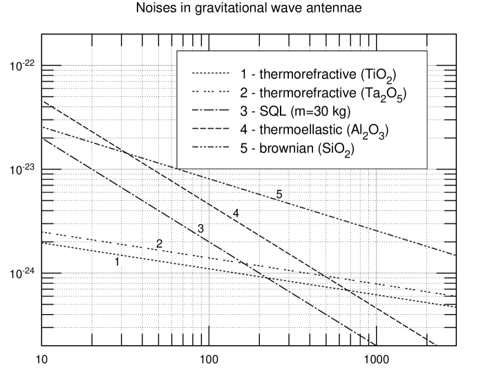
FIG. 1.: Comparison of SQL-limited sensitivity with different sources of noise in gravitational wave antennae: thermo-refractive, Brownian (dominating in fused silica mirrors) and thermo-elastic (dominating in sapphire mirrors).

III Numerical estimates

For the numerical estimates we assumed that the multilayer coating consists from alternating pairs of layers: $TiO_{2}$ ($n_{1}=2.2$) and $SiO_{2}$ ($n_{2}=1.45$), or $Ta_{2}O_{5}$ ($n_{1}=2.2$) and $SiO_{2}$ ($n_{2}=1.45$). The values of $\beta$ for $TiO_{2}$ and for $Ta_{2}O_{5}$ were found in [9].

We want now to compare the thermo-refractive fluctuations with thermoelastic noise (1) and noise associated with the mirrors’ material losses described in the model of structural damping[6] (we denote it as Brownian motion of the surface). In this model the angle of losses $\phi$ does not depend on frequency and for its spectral density the following formula is valid for infinite test mass [7, 1, 4]:

$$S^{\rm B}_{x}(\omega) \simeq \frac{4\kappa T}{\omega}\,\frac{(1-\sigma^{2})}{\sqrt{2\pi}Er_{o}}\,\phi,$$ (16)

where $E$ is Young modulus, and $\sigma$ is Poison ratio.

The spectrsal sensitivity of gravitational wave antenna to the perturbation of metric $h(\omega)$ may be recalculated from noise spectral density of displacement $x$ using the following formula:

$$h(\omega)=\frac{\sqrt{2(S_{x,\,r_{01}}(\omega)+S_{x,\,r_{02}}(\omega))}}{L},$$ (17)

where we used the fact that antenna has two arms (with length $L$) with two mirrors the fluctuations on which are averaged over the radii $r_{01}$ and $r_{02}$.

The LIGO-II antenna will approach the level of SQL, so we also compare the noise limited sensitivity to this limit in spectral form [8]:

$$h_{\rm SQL}(\omega)=\sqrt{\frac{8\hbar}{m\omega^{2}L^{2}}}.$$ (18)

For the calculations we used the set of parameters given in Appendix B (the same as in [1]) plus [9]

$$r_{01} = 3.6/\sqrt{2}\ \mbox{cm},\quad r_{02}=4.6/\sqrt{2}\ \mbox{cm},$$

$$n_{1} = 2.2,\qquad\beta_{2}=4\cdot 10^{-5}\ \mbox{K}^{-1}\quad(TiO_{2}),$$

$$n_{1} = 2.2,\qquad\beta_{2}=6\cdot 10^{-5}\ \mbox{K}^{-1}\quad(Ta_{2}O_{5}),$$

$$n_{2} = 1.45,\qquad\beta_{1}=1.5\cdot 10^{-5}\ \mbox{K}^{-1}\quad(SiO_{2}),$$

We used figures from [9] for ion plating method only, for other methods of deposition the value of $\beta$ may be two times larger. In figure 1 we plot all previously known noises [1] together with the new one. We see that thermorefractive noise limitation is close to SQL for the frequences near $200$ Hz.

Conclusion

Summing up, we may say that thermo-refractive effect is not small and it must be seriously considered in interferometric gravitational antennae (projects LIGO-II and especially LIGO-III, where overcomming of the SQL is planned). It is also important that this effect depends slower on the radii of the beam-spots than thermo-elastic noise and thus may become dominating for larger $r_{0}$ planned in LIGO-II and LIGO-III.

A

In this appendix we give the calculation of coefficient of reflection of light wave from multilayer coatings consisting of infinite sequences of pairs of quarter-wavelength dielectrical layers $n_{1}$ and $n_{2}$.

Let the refraction index of odd layers fluctuates on $\Delta n_{1}$ and the refraction index of even layers on $\Delta n_{2}$. One may reformulate this problem into the problem for distributed long line [5]. The equivalent impedance $Z$ of this system of layers may be deduced using the following statement: the addition of two layers does not change the value of $Z$.

Voltage $V_{2}$ and current $I_{2}$ at the end of second layer may be found from input voltage $V_{0}$ and current $I_{0}$ using transformation matrix $M$ ([5], formula (3.9.27)):

$$\left(\begin{array}[]{c}V_{2}\\ I_{2}\end{array}\right) = M\times\left(\begin{array}[]{c}V_{0}\\ I_{0}\end{array}\right),\quad M=\left(\begin{array}[]{cc}M_{11}&M_{12}\\ M_{21}&M_{22}\end{array}\right),$$

$$M_{11} = \cos\phi_{1}\cos\phi_{2}-\frac{n_{1}}{n_{2}}\sin\phi_{1}\sin\phi_{2},$$

$$M_{12} = -i\left(\frac{\sin\phi_{1}\cos\phi_{2}}{n_{1}}+\frac{\sin\phi_{2}\cos\phi_{1}}{n_{2}}\right),$$

$$M_{21} = -i\left(n_{2}\sin\phi_{2}\cos\phi_{1}+n_{1}\sin\phi_{1}\cos\phi_{2}\right),$$

$$M_{22} = \cos\phi_{1}\cos\phi_{2}-\frac{n_{2}}{n_{1}}\sin\phi_{1}\sin\phi_{2},$$

$$M \simeq \left(\begin{array}[]{cc}-\frac{n_{1}}{n_{2}}&i\left(\frac{\varphi_{2}}{n_{1}}+\frac{\varphi_{1}}{n_{2}}\right)\\ i\left(n_{2}\varphi_{1}+n_{1}\varphi_{2}\right)&-\frac{n_{2}}{n_{1}}\end{array}\right)$$

Here we take into account that for quarter-wavelength layers $\phi_{1}=\pi/2+\varphi_{1},\quad\phi_{2}=\pi/2+\varphi_{2}$ and therefore one may use approximation $\sin\phi_{1}\simeq 1,\quad\sin\phi_{2}\simeq 1,\quad\cos\phi_{1}\simeq-\varphi_{1},\quad\cos\phi_{2}\simeq-\varphi_{2}$.

Now we put that $I_{0}=YV_{0}$ and $I_{2}=YV_{2}$ ($Y=1/Z$ is generalized conductivity of the sequence of layers) and obtain two equations:

$$V_{2} = V_{0}\left(-\frac{n_{1}}{n_{2}}+iY\left(\frac{\varphi_{2}}{n_{1}}+\frac{\varphi_{1}}{n_{2}}\right)\right),$$ (A3)

$$YV_{2} = V_{0}\left(i\left(n_{2}\varphi_{1}+n_{1}\varphi_{2}\right)-Y\,\frac{n_{2}}{n_{1}}\right).$$ (A4)

Solving these equations we find conductivity $Y$ and reflection coefficient $K$:

$$Y \simeq -i\,\frac{n_{1}n_{2}}{n_{1}^{2}-n_{2}^{2}}\,\left(n_{2}\varphi_{1}+n_{1}\varphi_{2}\right),$$ (A5)

$$K = \frac{Y-1}{Y+1}\simeq-1-2i\,\frac{n_{1}n_{2}}{n_{1}^{2}-n_{2}^{2}}\,\left(n_{2}\varphi_{1}+n_{1}\varphi_{2}\right)$$ (A6)

From this point it is easy to obtain (2,3), assuming

$$\varphi_{1}=\frac{\pi}{2}\,\frac{\Delta n_{1}}{n_{1}},\qquad\varphi_{2}=\frac{\pi}{2}\,\frac{\Delta n_{2}}{n_{2}}$$

B Parameters

$$\omega = 2\pi\times 100\ \mbox{s}^{-1},\quad T=300\ \mbox{K},$$

$$m = =3\times 10^{4}\ \mbox{ g},\quad\lambda=1.06\ \mu,\quad L=4\times 10^{5}\ \mbox{cm};;$$

Fused silica:

$$\quad\alpha = 5.5\times 10^{-7}\ \mbox{K}^{-1},\ \ \lambda^{*}=1.4\times 10^{5}\ \frac{\mbox{erg}}{\mbox{cm s K}},$$

$$\rho = 2.2\ \frac{\mbox{g}}{\mbox{cm}^{3}},\ \ C=6.7\times 10^{6}\ \frac{\mbox{erg}}{\mbox{g K}},$$

$$E = 7.2\times 10^{11}\frac{\mbox{erg}}{\mbox{cm}^{3}},\ \ \sigma=0.17,\ \ \phi=5\times 10^{-8};$$

Sapphire:

$$\quad\alpha = 5.0\times 10^{-6}\ \mbox{K}^{-1},\ \ \lambda^{*}=4.0\times 10^{6}\ \frac{\mbox{erg}}{\mbox{cm s K}},$$

$$\rho = 4.0\ \frac{\mbox{g}}{\mbox{cm}^{3}},\ \ C=7.9\times 10^{6}\ \frac{\mbox{erg}}{\mbox{g K}},$$

$$E = 4\times 10^{12}\,\frac{\mbox{erg}}{\mbox{cm}^{3}},\ \ \sigma=0.29,\ \ \phi=3\times 10^{-9}.$$

REFERENCES

• [1] V. B. Braginsky, M. L. Gorodetsky, and S. P. Vyatchanin, Physics Letters A 264, 1 (1999); cond-mat/9912139;
• [2] A. Abramovici et al., Science 256(1992)325.
• [3] A. Abramovici et al., Phys.Letters.A 218, 157 (1996).
• [4] Yu. T. Liu and K. S. Thorne, submited to Phys. Rev. D.
• [5] S. Solimeno, B. Crosignani and P. Diporto, Guiding, Diffraction and Confinement of Optical Radiation, Academic Press, 1986.
• [6] P. R. Saulson, Rhys. Rev. D, 42, 2437 (1990);
G. I. Gonzalez and P. R. Saulson, J. Acoust. Soc. Am., 96, 207 (1994).
• [7] F. Bondu, P. Hello, Jean-Yves Vinet, Physics Letters A 246, 227 (1998).
• [8] V. B. Braginsky, M. L. Gorodetsky, F. Ya. Khalili and K. S. Thorne, Report at Third Amaldi Conference, Caltech, July, 1999.
• [9] Thin films for optical systems (for the International Journal of Optoelectronics), Ed: F Flory, Marcel Dekker Inc, ISBN 0 8247 96333 0, 1995.