Angular Structure of Lacunarity, and The Renormalisation Group

Abstract

We formulate the angular structure of Lacunarity in fractals, in terms of a symmetry reduction of the three point correlation function. This provides a rich probe of universality, and first measurements yield new evidence in support of the equivalence between self-avoiding walks and percolation perimeters in two dimensions.

We argue the Lacunarity reveals much of the Renormalisation Group in real space. This is supported by exact calculations for Random Walks and measured data for percolation clusters and SAW’s. Relationships follow between exponents governing inwards and outwards propagating perturbations, and we also find a very general test for the contribution of long range interactions.

]

In this letter we bring together two outstanding issues in the theory of fractals, which we believe will also have bearing on critical phenomena more generally. The first is ’Lacunarity’ [2, 3, 4], which as originally introduced could entail all the discriminations of fractal structure (beyond dimension) which are evidently visible yet hard to codify in a simple generic way. The second is the Renormalisation Group [1] which has been a predominant influence for three decades in the theory of critical scaling phenomena, fractals included, yet has never to our knowledge been regarded as a directly measurable object in its own right. Here we will present evidence and arguments that a particular version of Lacunarity measurement is effectively a measurement of the (Linearised) Renormalisation Group.

The ’Lacunarity Function’ was introduced [5] as a scaling reduction of the three point correlation function for a statistical fractal,

$${\cal L}(R,\theta)=\frac{C_{3}(\vec{r}_{1},\vec{r}_{2},\vec{r}_{3})}{C_{2}(\vec{r}_{1},\vec{r}_{2})C_{2}(\vec{r}_{1},\vec{r}_{3})}$$ (1)

where $C_{3}(\vec{r}_{1},\vec{r}_{2},\vec{r}_{3})$ is the conditional probability for points $\vec{r}_{2}$ and $\vec{r}_{3}$ to be occupied given that $\vec{r}_{1}$ is occupied, $C_{2}(\vec{r}_{1},\vec{r}_{2})$ the conditional probability for point $\vec{r}_{2}$ to be occupied given that $\vec{r}_{1}$ is occupied, and the Lacunarity Function ${\cal L}$ depends only on the angle $\theta$ between the two vectors $\vec{r}_{2}-\vec{r}_{1}$ and $\vec{r}_{3}-\vec{r}_{1}$ and their length ratio $R=r_{13}/r_{12}$.

The Lacunarity function defined above is (by construction) independent of absolute lengthscale and is a pure critical-point scaling object. It is crucial that we are discussing measurements averaged over an ensemble of fractal objects, or at least self-averaging over the interior of one object much larger than than both $r_{12}$ and $r_{13}$. The dependence of ${\cal L}$ on only a ratio of lengths follows from the assumption of continuous scale invariance, whilst the dependence on only a single internal angle follows in the more restrictive assumption that the ensemble of fractals in question has no favoured directions. The whole analysis presupposes the definition of some suitable measure for the fractal structure in question, but provided this is not multifractal [6, 7] any simple ambiguity in the measure is expected to cancel from the Lacunarity Function ${\cal L}$.

I The Angular Structure of Lacunarity

We introduce here the decomposition of the Lacunarity Function over angular harmonics, for example in two dimensions

$${\cal L}(R,\theta)={\cal L}_{0}(R)+2\sum_{m=1}^{\infty}{{\cal L}_{m}(R)\cos{m\theta}}.$$ (2)

Our physical interpretation of the individual components ${\cal L}_{m}(r^{\prime}/r)$ is that they measure the correlation between different lengthscales $r$ and $r^{\prime}$ of relative fluctuations, of a particular angular harmonic, in the local two point correlation about each mass point. They can be more precisely calculated as ratios

$${\cal L}_{m}(r^{\prime}/r)=M_{m}(r^{\prime},r)=\frac{<S_{m}(r^{\prime};\vec{r}_{1})S_{m}(r;\vec{r}_{1})^{*}>}{<S_{0}(r^{\prime};\vec{r}_{1})><S_{0}(r;\vec{r}_{1})>}$$ (3)

where $S_{m}(r;\vec{r}_{1})$ is the weighted count of occupied points within a shell of radius $r$ about mass point $\vec{r}_{1}$, each point weighted by the angular harmonic of its direction relative to $\vec{r}_{1}$ (i.e. ${\rm e}^{{\rm i}m\theta}$ in two dimensions), and the averages are with respect to all occupied mass points $\vec{r}_{1}$. [10]

The width of the shells used to compute the averages in (3) drops out of the result provided it is small enough, but with finite datasets some compromise must be made to obtain reasonable signal to noise ratio. We typically used shells of 7% width by radius. In the case of diagonal elements (only), that is $r=r^{\prime}$ equivalent to $R=1$, shot noise makes a systematically positive contribution to the reading for which we have corrected our data below.

Figure 1 shows contour plots of the shell mass correlations $M_{m}(r^{\prime},r)$ as a function of $ln(r)$ and $ln(r^{\prime})$ for a large site percolation cluster grown at criticality. The structure along the diagonal is direct evidence for the reduction $M_{m}(r^{\prime},r)={\cal L}_{m}(R=r^{\prime}/r)$ and on the basis of such plots we have averaged data parallel to the diagonal, within suitable looking windows, to obtain the curves for ${\cal L}_{m}(R)$ shown in figure 2.

Figure 3 shows a direct comparison between the corresponding measurements for the outer perimeter set of such a percolation cluster with those for a large self-avoiding walk. The broad agreement (with no adjustable parameters in any of the cureves shown) reinforces the claim that these two objects are in the same Universality Class, as very strongly suggested by Duplantier’s caclulation [8] of their identical $f(\alpha)$ spectra for the exterior harmonic measure.

II Connection to the Real Space Renormalisation Group

The physical idea behind the renormalisation group is that under critical conditions the structure of a system is propagated through a continuous cascade of length scales. This is usually viewed in terms of the propagation of certain (judiciously chosen) renormalised parameters which remain invariant at the fixed point. The linearisation of the renormalisation group about the fixed point then corresponds to the transmission of perturbations through the lengthscale cascade.

Our lacunarity function measures the correlation of structure fluctuations between different lengthscales and it is natural to suppose that this correlation arises due to propagation. If so, then our measurements of correlation directly probe the linearised renormalisation group. More strictly, we need the covariances rather than the correlations to probe propagation, to which end it is useful to distinguish from Lacunarity notation (and rescale) by writing

$${\cal LR}_{m}(R)=\frac{{\cal L}_{m}(R)-\delta_{m0}}{{\cal L}_{m}(1)-\delta_{m0}},$$ (4)

where we propose to take the liberty of refering to ${\cal LR}$ as the Local Renormalisation Group Function.

Our proposal is that if the local two point correlation function structure at radius $r$ about point $\vec{r}_{1}$ is perturbed $C_{2}(r)_{\vec{r}_{1}}\rightarrow C_{2}(r)(1+\epsilon_{m}(r;\vec{r}_{1})H_{m})$, where $H_{m}$ is a (normalised) angular harmonic, then the corresponding response at larger lengthscale $r^{\prime}$ should follow

$$\epsilon_{m}(r^{\prime};\vec{r}_{1})={\cal LR}_{m}(r^{\prime}/r)\epsilon_{m}(r;\vec{r}_{1}).$$ (5)

It is important to note that the Local Renormalisation Group Function defined above is a ’shattered’ response function, in that it gives the response due to changing the two point correlation at one locality. If we make a global relative perturbation $\epsilon_{m}(r)$ of the local two point correlation at lengthscale $r$ around every mass point, then the growth of corresponding response defines a “Global Renormalisation Group Function” ${\cal GR}$ through

$$\epsilon_{m}(r^{\prime})={\cal GR}_{m}(r^{\prime}/r)\epsilon_{m}(r).$$ (6)

From the number of (occupied) localities of radius $r$ contributing to perturbation in a larger vicinity of radius $r^{\prime}$, we expect the components of ${\cal GR}$ to scale as

$${\cal GR}_{m}(R)\simeq R^{D}{\cal LR}_{m}(R)$$ (7)

for a simple mass fractal of fractal dimension $D$. Note that only even $m$ are of physical consequence here, as the (global) two point correlation function is by construction an even function restricted to even perturbations.

An important consequence of equation (7) is that global perturbations are relevant at large lengthscales if the corresponding Local RG function falls off more slowly than $R^{-D}$ for large $R$.

The case of simple Random Walks in $d>2$ illustrates and tests these ideas with exact results. The general form of the Lacunarity function ${\cal L}(R,\theta)$ was first given in ref[5], but the angular harmonic decomposition of ${\cal LR}$ gives the much simpler form:

$${\cal LR}_{0}(R)=R^{2-d};\,\,{\cal LR}_{m}(R)=\frac{1+R^{2-d}}{2}R^{-m},\,\,m>0.$$ (8)

This gives ${\cal GR}_{0}(R)\simeq R^{4-d}$, ${\cal GR}_{2}(R)\simeq R^{0}$ and ${\cal GR}_{4}(R)\simeq R^{-2}$ for large $R$, which all have physical interpretation.

A negative $m=0$ perturbation at lengthscale $r$ means depressing the incidence of other points at radius $r$ from any given one, corresponding in polymer language to turning on some excluded volume. That the resulting perturbation at larger lengthscales $r^{\prime}$ grows as $(r^{\prime}/r)^{4-d}$ corresponds to the well known Fixman perturbation expansion of Coil Swelling[9]. The analogous positive perturbation leads to coil shrinkage (and ultimately collapse).

An $m=2$ perturbation corresponds to the local structure being stretched in some directions and shrunk in others, corresponding for a random walk to anisotropy in the individual walk steps. The scale independence of the resulting response follows from the equivalence of such random walks to affine deformations of isotropic ones, which we discuss as a much more general result below.

An example of an $m=4$ perturbation would be the intrinsic bias of random walks made on a square (more generally hypercubic) lattice, and the decay of the perturbation reflects the known irrelevance of this in the large lengthscale limit. Analogous interpretations apply to higher orders of lattice bias, for example $m=6$ and the triangular lattice in two dimensions.

An important issue is whether the propagation of perturbation is necessarily confined to running upwards in lengthscale. In systems governed by an equilibrium ensemble we can equally expect reverse (inwards) propagation governed by the form of ${\cal LR}$. Thus we are led naturally to predict that for every global perturbation propating outwards from $r$ to $r^{\prime}$ as $(r^{\prime}/r)^{-\sigma}$ there is propagation inwards of the same symmetry of perturbation from $r^{\prime}$ to $r$ as $(r^{\prime}/r)^{-\tau}$ where $\tau=\sigma+D$.

The corresponding inwards perturbations of a random walk can be identified. The zeroth harmonic corresponds to simple confinement (and checks out), whilst higher harmonics can then be interpreted in terms of the influence of a confining shape. The $m=2$ case, ellipticity, is particularly important because this corresponds to polymer elasticity.

Some of these interpretations can also be checked for less trivial fractals. For the Self Avoiding Walk (as for the random walk), the non-trivial part of the $m=0$ lacunarity is associated with the walk going from lengthscale $r$ out to lengthscale $r^{\prime}$ and coming back again. This is then governed by the probability of an SAW to close a loop, which is known to vary as $N^{-1}\propto{r^{\prime}}^{-D}$ where $N$ is the number of steps in the walk (to reach radius $r^{\prime}$). This leads to ${\cal GR}_{0}(R)\simeq R^{0}$ for large $R$, corresponding (correctly) to a change in the excluded volume causing the SAW to dilate uniformly on larger lengthscales. The inset in figure 3 shows our measured data for $L_{0}(R)-1\propto{\cal LR}_{0}(R)$ out to large $R$ and is consistent with $R^{-D}=R^{-4/3}$, albeit the data is noisy. The $m=2$ case for the SAW can be interpreted in terms of the scaling of elasticity for swollen polymers and leads to also to ${\cal LR}_{2}(R)\propto R^{-D}$ at large $R$; this checks quite well against the main data in figure 3.

We believe a very general result governs the $m=2$ lacunarity due to its RG connection, which explains why in all the fractals considered in this letter (numerically for the percolation cluster of figure 1, and analytically for random and self-avoiding walks),

$${\cal GR}_{2}(R)\simeq R^{0}.$$ (9)

This corresponds to the outwards global m=2 perturbation being marginally relevant, and it arises because a $m=2$ perturbation can always be accommodated by a global strain of the metric of space. This should of course fail when long range interactions are important, sensitive to the metric of distance, and therefore equation (9) serves as a general test of whether long range interactions play a role in the underlying physics.

III Concluding Remarks

We have presented arguments that the Lacunarity Function ${\cal L}$, or at least its asymptotes, can be viewed as response functions determined by the Renormalisation Group. It is harder to firmly establish just how much of the Renormalisation Group is thereby revealed. We can certainly restrict any such claim to the Linearised Renormalisation Group, because the Lacunarity Function can only probe fluctuation correlations about the critical point behaviour: in RG terms this means that it can only probe the vicinity of the corresponding fixed point. We have restricted our attention to simple mass fractals, directly characterised in terms of one (positive definite) scalar field, the mass density. We speculate that ${\cal L}$ incorporates all the linearised RG relating to how this field might be coupled locally and bilinearly to itself, whereas it cannot know anything about what happens when other fields are introduced.

A rich range of issues remain to be explored. We already mentioned that the odd angular harmonics in the Lacunarity Function lack a simple Response Theory interpretation because the two point correlation function must be even. One way to deal with this is to recognise more explicitly the way the Lacunarity Function depends only on the shape of the triangle of points it correlates, which leads to a parameterisation of ${\cal L}$ involving only even harmonics; all the odd harmonics are thereby related to the even ones. However it is more interesting to consider structures from irreversible growth where correlating present with future growth is the natural correlation to investigate and odd harmonics are no longer forbidden in such time resolved correlations. We anticipate that problems like the response of Diffusion Limited Aggregation to anisotropy should be analysed in this way.

In principle our work opens the door to measuring the Renormalisation Group, via Lacunarity, directly from real experimental data (as opposed to just computer simulations). We recognise, however, that this may not be easy. Our simulations span some three decades of lengthscale (i.e. cluster radii of order 1000 units), and even then the match up to expected scaling laws is not always good. The best way forward would appear to be not to target the asymptotic exponents, but rather to compare absolute lacunarity values between experiment, simulation and theory at moderate $R$. On the theory side, our exact Random Walk results are extendable to Markov Chains, but no other exact results are known (other than exponents).

Finally, whilst all the fractals discussed in this letter have close relation to equilibrium critical phenomena, our present definition of Lacunarity certainly does not extend trivially to critical phenomena in general. We believe the correct analogue of our three point correlation for a mass fractal is a four point correlation of the corresponding critical distributions, the extra point being at infinity. The natural generalisation of our lacunarity function to spin models would thus be in terms of a four point correlation function at the critical point, and we look forward to exploring this in future work.

IV Acknowledgements

This work was supportred by EPSRC, grant GR/L55346, and by the EU under TMR contracts ERBFMBI-CT97-2746 and FMRX-CT98-0183.

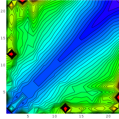
FIG. 1.: Contour plot of the cross correlation of local two point function between different lengthscales, as per equation (3) with $m=0$, for a percolation cluster of $1.5\,10^{6}$ sites grown on a traingular lattice at the percolation threshold. The axes are labelled proportional to the logarithm of the two lengthscales correlated. Contour lines parallel to the diagonal correspond to this reducing to a scale invariant ’Lacunarity Function’ depending only on the lenghtscale ratio. Scale invariance breaks down around the edges of the plot where one lengthscale approaches either the lattice spacing or the sample size.

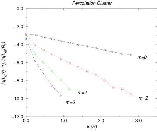
FIG. 2.: The different angular harmonics of the Lacunarity Function for the two dimensional percolation cluster of figure 1. The $m=0$ data correspond to the central part of the contour plot averaged parallel to the diagonal, and the other harmonics are defined analogously in equation (3)

.

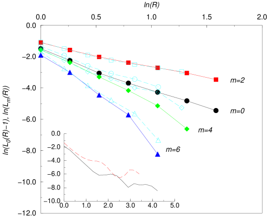
FIG. 3.: Angular harmonics of the Lacunarity Function compared between the Outer Perimeter of a Percolation Cluster (as per figure 1) and a Self-Avoiding Walk (in two dimensions) of comparable size. The general agreement of these measurements, which contain no adjustable parameters, supports both types of object being in the same unversality class. The inset shows the data for the zeroth harmonic extended to larger lengthscale ratios.

REFERENCES

- [1] See L.P.Kadaoff, Statistical Mechanics, Scaling and Renormalization, World Scientific (1999) and references therein.
- [2] B.B. Mandelbrot, The Fractal Geometry of Nature, Freeman San Francisco (1982).
- [3] Y.Gefen, B.B. Mandelbrot and A. Ahrony, Physical Review Lett. 45, 855 (1980).
- [4] Y.Gefen, A. Ahrony and B.B. Mandelbrot, Journal of Physics A 17, 1277 (1984).
- [5] R.Blumenfeld and R.C.Ball, Physical Review E 47, 2298 (1993).
- [6] B.B. Mandelbrot, Comptes Rendus (Paris) 278A, 289-92 & 355-8 (1974).
- [7] T.C. Halsey, P. Meaking and I. Procaccia, Physical Review Lett. 56, 854-7 (1986).
- [8] B. Duplantier, Physical Review Lett. 82, 3940-3 (1999).
- [9] M. Fixman, J. CHem. Phys. 23, 1656 (1955).
- [10] For a fractal represented by mass points, the direct cost of this operation is Order unless coarse graining economies are used.