A quantum Monte Carlo study of the one-dimensional ionic Hubbard model
Abstract
Quantum Monte Carlo methods are used to study a quantum phase transition in a D Hubbard model with a staggered ionic potential (). Using recently formulated methods, the electronic polarization and localization are determined directly from the correlated ground state wavefunction and compared to results of previous work using exact diagonalization and Hartree-Fock. We find that the model undergoes a thermodynamic transition from a band insulator (BI) to a broken-symmetry bond ordered (BO) phase as the ratio of is increased. Since it is known that at the usual Hubbard model is a Mott insulator (MI) with no long-range order, we have searched for a second transition to this state by (i) increasing U at fixed and (ii) decreasing at fixed U. We find no transition from the BO to MI state, and we propose that the MI state in is unstable to bond ordering under the addition of any finite ionic potential . In real 1D systems the symmetric MI phase is never stable and the transition is from a symmetric BI phase to a dimerized BO phase, with a metallic point at the transition.
I Introduction
Strongly-correlated systems of interacting electrons lead to many of the most interesting phenomena observed in solid state physics[1]. As a function of the interaction strength, there can be quantum phase transitions [1] characterized by an order parameter with the possible development of long-range order and a transition to a broken symmetry state. Interactions can also lead to “Mott insulators” (MI) and to metal-insulator transitions [2]. An important question is whether or not in the thermodynamic limit a Mott insulator must be associated with a phase transition that is accompanied by a broken symmetry and a corresponding order parameter. In his original work, Mott [3] argued that the insulating character did not depend upon an order parameter. On the other hand, Slater [4] emphasized the relation of the insulating behavior to the long range order, and in many cases it is known that the MI state must be accompanied by a broken symmetry[5].
To address such issues theoretically we must have methods that can clearly distinguish metals from insulators, i.e., the ability to transport charge[6, 7, 8] vs. localization of the electrons[8]. Insulators at absolute zero can not transport arbitrary amounts of charge macroscopic distances across their bulk; however, the center of electronic charge can shift in response to external fields, which is described in terms of changes in polarization[6, 7]. The polarizability is characterized by the degree of electronic delocalization[8] which increases with the proximity to the metallic state. Recently, there have been new developments defining macroscopic polarization and localization in terms of the insulating ground state wavefunction[9, 10, 11, 12, 13, 14, 15]. These theories formulate the polarization and localization in terms of Berry’s phases [16] which can be calculated using “twisted boundary conditions” or in terms of the expectation value of an exponentiated operator. Such twisted boundary conditions have been applied in the past to study metals and approach metal-insulator transitions from the metallic side[17, 18, 19, 8]. With the recently developed methods for insulators, there are now complementary tools[15] to provide quantitative information on the divergence of the localization length as one approaches the metal-insulator transition from the insulating side.
Generalized Hubbard models [20, 21] are well-suited for studies of fundamental issues regarding metals and insulators because they are simple models that exhibit a wide range of behaviors depending upon the parameters in the models. The simplest of all, the original Hubbard model with an on-site interaction and nearest neighbor hopping in , was solved exactly by Lieb and Wu [22]. Their paper, entitled “Absence of Mott Transition …”, conveys the point that there is no change of spatial symmetry and no phase transition at any positive U. At half-filling the model is metallic at , whereas at any positive interaction U a gap exists to charge excitations but no gap exists to spin excitations. This is commonly referred to as the MI state, but in this case there is no “Mott transition”. At any other filling, the model is always metallic. There is never a state that would be called an ordinary band insulating (BI) state. However, in systems of higher dimensionality (), a MI state is always accompanied by a broken symmetry[5].
Many new possibilities emerge for generalized Hubbard models in . The ionic D Hubbard model with two inequivalent sites, proposed by Nagaosa[23] and later by Egami[24] as a model ferroelectric, is ideal for studying how quantized particle transport is modified by electron correlation in a many body system. On general grounds we expect a transition to occur from an ionic band insulator to a strongly correlated Mott insulator as is increased. Evidence for such a transition was found in exact-diagonalization calculations[13, 10], where the electronic polarization was found to jump abruptly between two discrete values fixed by the existence of two centers of inversion at the two sites. Such behavior has been termed a “topological transition” [14] that occurs in finite systems and therefore is distinct from a true quantum phase transition. These solutions predict that the model has a metallic point separating two insulating phases and that a ferroelectric polarization results only if the atomic sites are displaced from the centers of inversion.
However, recently Fabrizio, et al.,[25] have proposed that this model will instead exhibit two quantum phase transitions: one from a BI state to a long range bond ordered (BO) state, predicted to be in the Ising universality class, and a second from the BO to the MI state, predicted to be a Kosterlitz-Thouless transition. Such transitions to BO states have recently been found in D Hubbard models with extended interactions (U-V) by Nakamura.[26] The BO state is a broken symmetry state in which the system becomes ferroelectric due strictly to electron-electron interactions even if all the atoms are at centers of inversion.
During the course of the present work, two preprints have reported calculations of charge and spin gaps in the model[27, 28]. Even though each work uses the density matrix renormalization group (DRMG) that allows studies of very large 1D systems, each group reports great difficulty in extrapolating to large size the small spin gaps and the two papers come to opposite conclusions regarding the existence of the BO state.
The purpose of this paper is to study the ionic Hubbard model using a method that (i) will treat electron correlation exactly and (ii) scale to large systems needed to treat systems near second-order phase transitions. For these reasons we use quantum Monte Carlo [29](QMC) which in principle is exact since there is no “fermion sign problem” in this particular D model (so long as there is non-zero overlap between our trial function and the true ground state). To our knowledge this is the first QMC study of polarization and localization in any system, and the first study of the ionic Hubbard model with systems large enough to determine quantitatively the nature of the transitions and whether or not there exists the spontaneously bond-ordered phase proposed by Fabrizio, et al.[25]. Furthermore, if there are indeed quantum phase transitions in the ionic model – whereas it is known that there are none in the usual non-ionic Hubbard model – then it follows that one must address the issue: Is a critical degree of ionicity required, or is the usual Hubbard model unstable to infinitesimal ionic perturbations? It is known [30, 31, 32, 33, 34] that the usual Hubbard model is unstable to dimerization at all . Thus a second question is: does this instability play a fundamental role in stabilizing the bond-ordered state?
The organization of the paper is as follows. In Sec.II, we introduce the model studied in this paper. In certain cases, depending upon the parameters of the Hamiltonian, this model is exactly soluble. We discuss the relevance of these solutions to the more general case studied in this paper. In Sec. III formulas for evaluating the electronic polarization and localization are presented. In Sec IV, we introduce the Quantum Monte Carlo (QMC) methods employed to evaluate expectation values and we describe their respective limitations. These are Variational and Green’s Function Monte Carlo algorithms and the “forward walking” method for computing expectation values of operators that do not commute with the Hamiltonian. Our results are presented in Sec. V and comparisons are made with previous studies using exact diagonalization and Hartree-Fock. In Section VI, we discuss the differences between our results and previous studies and the consequences of our new findings.
II The Model
The generalized ionic Hubbard Hamiltonian [23] is defined by
| (1) |
where is the Hamiltonian of the usual Hubbard model
| (3) | |||||
Here creates (destroys) an electron of spin on site while is the density operator of electrons of spin on site . This system is an idealized model of a chain of atoms that can have at most electrons of opposite spin per atom. The magnitude of the matrix element () controls the strength of covalency in the centrosymmetric lattice and determines the width of the energy band in the non-interacting limit. Interactions are included only for electrons that occupy the same site, and the strength of electronic correlation is determined by the ratio of .
The ionic term,
| (4) |
consists of an on-site energy() that alternates between neighboring sites, which is intended to model the electrostatic potential of cations and anions in an ionic material. By adjusting the ratio of , we can vary the degree of covalency and ionicity to levels similar to those of real insulating systems.
Although we will not study dimerization, per se, it is crucial to include a dimer term that breaks the inversion symmetry and is defined with the Su-Schrieffer-Heeger form[35]
| (5) |
Here denotes a dimerization term in the Hamiltonian () that incorporates the effect of alternately displacing the atoms from their equilibrium positions () and is the linear electron phonon coupling constant. The operator is the “bond order” operator
| (6) | |||||
| (7) |
which is a staggered hopping operator, the expectation value of which is the average difference in kinetic energy associated with the two bonds in a unit cell. Here is the number of sites, , the number of cells, and the strength of the bond. (Fabrizio, et al., refer to this as a “dimerization” operator; however, we will use the term “bond order” [26], since it denotes a property of the electronic state and may occur even if the lattice is not dimerized.)
Exact analytic solutions for Eq. 1 exist in several limiting cases. In the non-interacting case (), the electrons fill the lowest energy band (E(k))
| (8) |
up to the Fermi k-vector . In the case there is no gap at the Fermi surface and the system is metallic, but for any finite or a gap is opened at the Fermi surface and the system is a band insulator. If and we perturb the system by adjusting the lattice is known to suffer the famous Peierls instability [36, 37] and energetically favors dimerization.
Exact solutions in the presence of correlation () are restricted to cases in which (i) there is no intrasite coupling (); (ii) there is a large displacement such that and the lattice is completely deformed into an array of independent dimers; or (iii) the case of the usual Hubbard model where there is no ionic potential or lattice deformation () for which there are exact analytic solutions for all [22]. In the last case, the exact solution predicts that at half-filling the system becomes a Mott insulator for any non-zero . There is no change of symmetry from the case of (which is a metal) and at “very large” the system reduces to the Heisenberg spin model, which also has no long range order or spin gap in one dimension. For large the exchange coupling of the mapped spin model is . The MI and BI regimes are commonly distinguished from one another in literature on the basis of spin-charge separation [38]. In both cases there is a gap to charge excitations but in the MI state the spin gap is zero while in the BI state both spin and charge gaps are non-zero.
The limiting cases (i) and (ii) are also instructive for our purposes. In the former () there is a transition at from a singlet state with two electrons on the site with on site energy , which is like a band insulator, to a state with one electron per site which has a spin on each site and is like a Mott insulator. Thus one might expect a transition from the BI state to some other phase as is increased even if . The second case (ii) with and always leads to a singlet ground state for the isolated dimers, which relates to the known result that one has a singlet state with a gap for both spin and charge excitations for any degree of dimerization. Thus one can ask: does a transition occur from the BI to MI regime as for ? Is there a spontaneous[25] bond-ordered phase? We shall test these ideas with our QMC simulations applied to the general case where there are no exact analytic solutions.
III Electronic Polarization and Localization
The issues associated with calculating the electric polarization in an extended system have a long, torturous history[39, 40]. Only recently have formulas been devised that express the polarization and localization of electrons directly in terms of the ground state wavefunction[9, 10, 40]. One type of formulation measures the change in polarization as a Berry’s phase obtained by integrating over twisted boundary conditions and an adiabatic parameter that characterizes the evolution of the system as it moves from one state to another[9, 10]. This approach has also been extended to localization in an independent particle formulation[41] and recently in a many-body formalism[15]. An alternative approach has been developed by Resta and Sorella[11, 12] and others[14, 15], who expressed the electronic polarization and localization in terms of the expectation value of a complex operator
| (9) |
where the average is taken with respect to a truly correlated many body wavefunction utilizing periodic boundary conditions (PBC) sampled using one of the quantum Monte Carlo techniques discussed in section IV. In terms of the polarization of the many body ground state can be expressed as
| (10) |
and a measure of the electronic delocalization is given by
| (11) |
These expressions are exact only in the limit of an infinitely large system, and in practice one measures each for increasingly larger supercells until convergence is met. Recently Souza et al [15] have shown that Eqs 10 and 11 are in fact valid in a correlated many-body system and related this formulation to that using twisted boundary conditions. They also demonstrated that the formulas relate directly to measurable fluctuations of the polarization, thus validating the two formulas as direct measures of electronic polarization and delocalization.
To our knowledge the present work is the first study of polarization and localization on large systems with fully-correlated many-body wavefunctions sampled using QMC. Previous work has been limited to exact diagonalization studies on small systems or mean field methods such as DFT and HF. For our work we use quantum Monte Carlo methods techniques with Eqs 10 and 11 because these are directly in the form of expectation values of quantities using wavefunctions that have the usual periodic boundary conditions. This is a great advantage in QMC since we can use the same methods developed for other problems [29]. The approach using twisted boundary conditions would require a change in the algorithms, in particular the adoption of a “fixed-phase”[42, 43] rather than a fixed node method. Such an approach would have important advantages, the most significant that it would allow calculations of polarization and localization to be done on smaller supercells[15]. There are other reasons that we prefer to use the standard boundary conditions: we shall see that very large cells are readily handled in QMC and furthermore the ability to work with large systems is very important in conclusions on the nature of the phase transitions in this study.
IV Quantum Monte Carlo
Quantum Monte Carlo (QMC) methods [44, 29] make it possible to evaluate expectation values of operators in many-body systems by stochastically sampling a probability distribution. In this paper we focus on two methods, Variational Monte Carlo (VMC) and Greens Function Monte Carlo (GFMC), that can be used to determine properties at temperature equal zero. The space of integration () is the set of all the electronic coordinates , which is sampled by “walkers” which denote a set of configurations . A random walk is generated by starting from an initial configuration , from which new configurations are generated by successively stepping to new random configurations, e.g., using a generalized Metropolis method [45]. This is done by accepting or rejecting new configurations at each step based upon a chosen acceptance function (). After a period of time the walk will stabilize such that the set of configurations visited will be distributed according to . VMC measures expectation values by uniformly averaging over the configurations visited by the Metropolis algorithm where as in GFMC the average is weighted according to .
A Variational Monte Carlo
VMC measures expectation values of a variational trial wavefunction ( ), where denotes a set of parameters that can be optimized. Averages for an arbitrary operator are obtained by sampling
| (12) | |||||
| (13) |
the local form of , defined as , over a set of points () distributed according to the modulus of the wavefunction. The are obtained by choosing as the acceptance function in a generalized Metropolis algorithm. VMC is easy to implement but is limited in accuracy by the form of the adopted wavefunction. In our work has the Gutzwiller form[46]
| (14) |
which is a product of Slater determinants for each spin (thus guaranteeing that the wavefunction is anti-symmetric) and a two body Jastrow correlation function that reduces the amplitude of configurations with doubly occupied sites for , thus lowering the interaction energy. The single body portion of Eq. 1 is parameterized by and , which means the orbitals used to construct the Slater determinants are obtained by diagonalizing the non-interacting () portion of the Hamiltonian () and adjusting () to optimal values that minimize the energy in Eq. 13 wrt. .
B Green’s Function Monte Carlo (GFMC) for Discrete Systems
GFMC starts with the optimized VMC wavefunction upon which a projection is applied to obtain an improved ground state. To illustrate the principles upon which this method depends, one can expand in terms of the eigenstates of . Then the imaginary time propagator acting upon has the form
| (15) |
Note that the exact ground state, , can only be obtained so long as it has non-zero overlap with .
The following is a summary of the method developed by Haaf et al [47] some of which is used in the next section. For lattices this projection scheme takes advantage of the fact the spectrum of is bound such that one can use a Green’s function projection with no finite-time-step error [48]
| (16) |
The propagator acting upon the trial wavefunction now becomes
| (17) |
By inserting the identity operator in the real space configuration basis ()
| (18) |
between successive applications of the projection operator and multiplying both sides by
| (21) | |||||
we obtain an expression for the wavefunction after steps in imaginary time. If the time step is sufficiently small and can be interpreted as a probability. Using this probabilistic interpretation, the sum in Eq. 21 above is evaluated using Metropolis. Multiplying and dividing by , Eq. 21 above can be importance sampled [44] as
| (23) | |||||
where
| (24) |
Since the are not normalized to one, they can not be interpreted directly as a probability. This is remedied by expressing as
| (25) |
where is identified as the probability of moving from to and given by
| (26) |
while the weight normalizes p such that and is
| (27) |
The nodal structure of the ground state divides configuration space into regions in which is positive or negative, so that changes sign upon crossing the nodal surface in configuration space. Crossing the nodal surface by a walker causes difficulties in Monte Carlo sampling since the weight of a walker must be positive definite if it is to be interpreted in a probabilistic manner. In general, one must make some approximation to remedy this problem, by fixing the sign of in the Monte Carlo sampling; this is referred to as the ”fixed node approximation”, which has been described for lattice problems by ten Haff, et al.[49]
In the generalized Hubbard model considered here, QMC is exact because: (i) the only nodes of the ground state wavefunction are the points where two electrons of the same spin cross, (ii) the nodes are the same as in the trial function which automatically obeys this condition, and (iii) the Monte Carlo sampling is restricted to a nodal region in which the sign of is fixed. The last condition is realized in the present work because each move involves only one electron moving one site at a time; we never reach the nodal surface since neighboring in which a site is doubly occupied by two electrons of the same spin are not allowed. Thus our algorithm samples one nodal region (either positive or negative) which is sufficient, since they are identical due to the antisymmetry of the wavefunction.
Implementation of the above method is as follows. A VMC calculation is performed which supplies a number of walkers initially distributed according to . Each of these are then randomly walked along a path in configuration space using as the Metropolis acceptance function of moving from to . Each step is weighted by such that the walker’s accumulated weight is
| (28) |
Expectation values for an arbitrary operator after projections of the green’s function are measured by averaging the weighted local form of of each walker
| (29) |
Averages in GFMC equal the ground state expectation value only for those operators which commute with because the inner product Eq. 29 is a “Mixed Estimator” between and . Operators that commute with share the same eigenstates and the operator in Eq. 29 can be considered to act to right on , thus returning the ground state and cancelling the normalization of the denominator. Conversely operators that do not commute with have different eigenstates and thus do not cancel the normalization of the denominator in Eq. 29. Consequently GFMC does not produce exact results for these operators; such expectation values will be addressed later.
C Test of GFMC on Ordinary Hubbard Model
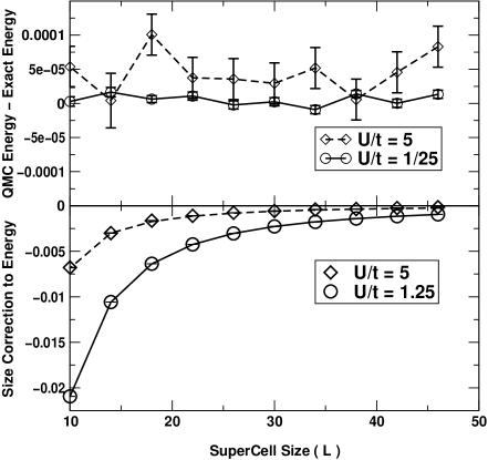
The accuracy with which the energy can be measured in GFMC and the magnitude of finite size effects can be addressed by comparing with exact results for the usual Hubbard Model at filling, which have been evaluated by Hashimoto [50] for finite systems of sites using periodic boundary conditions. In Fig 1 the differences in energy between lattices of size and the thermodynamic limit is plotted for two cases . The finite size effects at typical are of order for a supercell of sites. Thus we do not anticipate any difficulty in calculating the energy except in cases where there is a much longer correlation length than in the usual Hubbard Model, e.g., near a phase transition where correlation lengths diverge.
D Stability of the Ordinary Hubbard Model ()
For comparison to our work later it is useful also to study the dimerized Hubbard model with . Work on related issues in the past two decades has verified early theoretical predictions [30] that electron correlation enhances the Peierls instability of the non-interacting Hubbard model as . Using the Hellman-Feynman theorem the bond order can be identified as the first derivative of the energy wrt the lattice distortion or . The bond order susceptibility or the second derivative of the energy wrt. has a logarithmic divergence as [37], which is referred to as the Peierls instability. The energy near varies as [51]
| (30) |
where the amplitude and are dependent upon the strength of electron correlation. For is proportional to and , and for variational methods suggest the same results. In the strongly correlated regime the lattice can be mapped onto a Heisenberg lattice where is proportional to and . Although the instability is enhanced at large U, the effect is more difficult to observe since the electronic energy is much smaller.
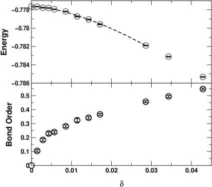
In our studies we consider small ionic deviations () from the usual Hubbard model for . The QMC energy and bond order are plotted vs in Fig 2 for an site lattice. The GFMC energy was fit to Eq 30 using a non-linear least squares routine. The parameters of the fit are , , and and give a reduced chi square of . This data agrees quite will with that of Black and Emery [52] who observed in the Heisenberg model. The energy of the symmetric lattice is within error bars of the exact thermodynamic limit of . The divergence of the lattice’s susceptibility of the lattice to bond ordering can be observed in Fig 2; as the level of distortion approaches zero the bond order approaches the origin with infinite slope.
E Expectation Values and Forward Walking
As noted before, GFMC does not produce exact expectation values for operators that do not commute with . There are several ways to improve upon the GFMC mixed estimator for such expectation values. One is an approximation that is valid so long as the VMC and GFMC averages are close to one another. Expressing as and taking the inner product, the ground state expectation value can be expressed as[44]
| (31) |
However, this approximation breaks down whenever the VMC trial wavefunction is not a good approximation to .
The exact ground state expectation value of any operator () can be found if the mixed expression Eq. 29 is replaced by one involving the exact wavefunction in both the bra and ket
| (32) |
This can be accomplished by “forward walking” [44], which can be simply expressed in terms of the GFMC method previously discussed. The same methods and terminology used in GFMC are also applicable here. Inserting the identity operator between each projection and using importance sampling Eq. 32 can be rewritten as
| (34) | |||||
The are sampled as before in terms of a probability function () and weight (). A series of walkers, initially distributed according to the VMC trial function, are stepped along paths () in configuration space by Metropolis sampling. After projections the accumulated weight of each is the product of all steps weights, as defined in Eq. 28. The walkers weights are distributed according to the mixed probability distribution . The local form of ( is measured for each walker but not averaged as it is in GFMC. The walkers are moved an additional steps in imaginary time over which they accumulate post measurement weights (). Averages are computed using each walkers accumulated weight before and after measuring
| (35) |
Although this method is in principle exact, assuming the nodal structure of is known, it also has its disadvantages. In particular, the width of the post-measurement weight distribution grows with the number of steps , thereby increasing the fluctuation of the forward walking estimates. To achieve a desired level of accuracy additional measurements are needed but the error in QMC decreases inversely with the square root of their number. Consequently, to obtain the same error as that in GFMC, forward walking may require many times more estimates in Eq. 35. This is the limiting factor in applying forward walking.
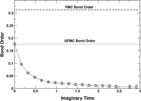
To illustrate the practicality and usefulness of this method, we show in Fig 3 the bond order as a function of forward walking for the centrosymmetric lattice at , and sites. We have chosen a poor trial wavefunction biased towards bond ordering by defining the determinant part of the wavefunction Eq. 14 using a Hamiltonian with . At this particular the system is a band insulator (as shown below), consequently the bond order must be zero; however, the average bond order in VMC and GFMC is non-zero as a result of using this trial wavefunction. The VMC expectation value of the bond order is substantially different from and reflects the poor quality of the trail state; whereas the GFMC average is closer to the exact result but remains far from satisfactory. The results in Fig 3 illustrate the strengths and weaknesses of forward walking. The key point is that there is a competition between the improvement of the estimate and the growth of the statistical errors with projection time. As shown in the figure, the method vastly improves the results even for very poor wavefunctions without the proper symmetry. In general, we use much better trial wavefunctions, and so the convergence to the exact result in our work below is more rapid than that depicted in Fig 3.
V Results for Ionic Hubbard Model
The unit cell for the ionic Hubbard model is composed of sites and the Hamiltonian is given in Eq. 1. In order to understand the meaning of the polarization and bond order in this system, it is helpful to consider first the non-interacting case with , where one can visualize the electronic properties in terms of Wannier functions. At zero dimerization () the Wannier functions are centered on the sites whose onsite energy is shifted by and . The electrons of opposite spin in each unit cell both occupy the lowest energy Wannier function centered on the lower energy site. In the dimerized lattice (), the centers are displaced from the sites. The magnitude of dictates the amount by which they are off center from the lowest energy site while sign of determines whether the center is to the left or right of this site. Strictly speaking the existence of Wannier functions in correlated systems () has yet to be proven but we will continue to use the concept of the center of the localized states for illustrative purposes. As U increases the electrons find it energetically undesirable to occupy the same site, and in the dimerized state the center of the distribution shifts further away from the low energy site. The limit of this displacement (i.e., polarization) is since one would never favor having more than one electron on the higher energy site. Similarly, the limit of the bond order is corresponding to isolated dimers.
As there are only three possibilities. If there is a spontaneous breaking of the inversion symmetry the polarization can assume any fractional value between 0 and 1/2. If there is no breaking of symmetry, there are still two possibilities since there are two centers of symmetry: the polarization can be 0 or 1/2. If the reference point defined to be zero is the usual band insulator where both electrons occupy the Wannier function centered on the lower energy site, it has been proposed[13, 53, 54] that P = 1/2 corresponds to a Mott insulator with no long range order.
We first report results of our study of the ionic Hubbard model with parameters fixed at the values used in previous work[13, 53, 54], so that direct comparisons can be made. The energy scale is set by defining , and . The previous conclusions with which we will compare are based upon exact diagonalization of the many-body Hamiltonian in small supercells[13, 54] and Hartree-Fock calculations[53]. The study[13] using exact diagonalization of site lattices with twisted boundary conditions found a jump of in the electronic polarization for , i.e. an electron in each unit cell being transported lattice constant, at a critical value of (). This was interpreted as a transition between BI and MI phases, which was supported by Hartree Fock (HF) calculations that showed similar behavior at . Extrapolations using larger cells of sites[54] find , presumably a more converged value. The key points are: (i) the transition point is found to be a metallic point with divergent delocalization; (ii) effective charges diverge and change sign at the transition; and (iii) there is no sign of the bond-ordered state predicted by Fabrizio, et al.[25]. This new state would have long range order and break the inversion symmetry of the lattice, thus allowing the polarization to take any fractional value.
The present work is based upon the QMC algorithms described earlier and the formulas for polarization and localization in section III. The first step in applying the QMC methods is to find a trial wavefunction that has as much overlap with the true ground state as possible. This is achieved by optimizing the parameters to minimize the energy. To determine the optimal value of we have used a newly devised technique that significantly reduces the amount of computational effort required [55]. Using the optimal Gutzwiller parameter the energy of for different and is sampled using VMC. We adjust and to lower the VMC energy and measure it at several points in the neighborhood of its minimum. A curve fit is then performed using these points to determine the optimal and .
A Comparison with Exact Diagonalization and Hartree-Fock
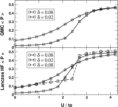
Previous studies distorted the lattice by varying degrees and these results provide a basis of comparison with QMC. We have measured the polarization of the ionic lattice for large () and small () lattice distortions and plotted these with the corresponding results of previous studies in Fig 4. Size effects are accounted for by extrapolating to the thermodynamic limit in ; this will be outlined more clearly in the following section. The Lanczos results agree well with those of QMC for considering the fact they were obtained using site supercells with twisted boundary conditions. This is in agreement with previous studies using exact diagonalization [32, 51] on the usual Hubbard model which found that small cells of this size were sufficient to reach thermodynamic convergence in the regime, whereas convergence with cell size is worse for smaller . (The jump in the polarization found in HF calculations for non-zero is unphysical and arises because the mean field approximation leads to an anti-ferromagnetic ground state. In this is strictly prohibited because quantum fluctuations are strong enough to destroy long range order in any continuous quantity.) As the magnitude of the distortion () approaches the difference between QMC and Lanczos becomes greater. Studies using exact diagonalization and HF observed that the polarization as a function of tended to below a critical and above it; consequently the dynamic charge was observed to change sign upon crossing this critical point. In the lower plot of Fig 4 this is exhibited as a crossing of the curves for . On the contrary we observe that the dynamic charge remains the same sign for the entire range of studied (except that the sign of is difficult to establish for large where it is near zero). This difference is attributed to the fact that for small and for near the electrons are very delocalized and correlation lengths exceed the cell size[15]. Integrating over twisted boundary conditions provides thermodynamically quenched expectation values so long as the Wannier functions of the eigenstates have vanishing overlap. Near the critical point the , obtained by exact diagonalization of and site rings, do overlap significantly; consequently, regardless of the number of k-space points averaged over by Resta and Sorella, the polarization will not converge to that of QMC.
The average polarization in Fig 4 was measured using forward walking. For the polarization at these values of , forward walking is not essential and the same results can be obtained using Eq 31. However, localization is more sensitive to inaccuracies in the wavefunction and accurate expectation values are provided only by using forward projection even at these relatively large values of . As the level of dimerization is reduced such that the extrapolation technique breaks down and only forward projection can provide accurate estimates for polarization and localization. Consequently we only report in this paper those QMC results obtained using forward projection.
The observation of a topological transition in the work of Resta and Sorella, and Guidopoulos, et al., is based upon their finding that as the polarization jumps discontinuously from 0 to 1/2 at a critical (or ). This means that the dynamic charge (), defined as , diverges and changes sign at as . In latter work [12] Resta and Sorella showed that is a metallic point where the electronic localization length () diverges, and Guidopoulos, et al., found energy gaps that extrapolated to zero. We will compare these results with our work below.
B Phase transition to Bond-ordered State
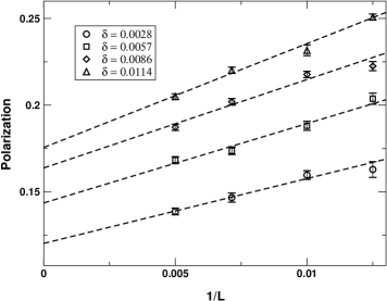
We have measured the forward walking estimators for , and and taken the limit of to study the nature of the quantum phase transition. The formulas used to obtain expectation values for polarization and localization are only accurate in the limit . This limit is taken by fitting measurements at finite to a linear least squares fit in and extrapolating to . We have found to accurately account for the finite size effects of and for . This scaling has only been found appropriate upon increasing the supercell size above a critical threshold which depends on the proximity of the metallic state. The accuracy of the finite size corrections to are illustrated in Fig 5 at for different magnitudes of . The data in Fig 5 was collected near the critical point of the phase transition, where size effects are large and must be treated accurately. If the system is sufficiently far from such a critical point, size effects are less pronounced and there is a more rapid convergence to the thermodynamic limit.
Using the infinite estimates for the polarization and localization on lattices dimerized by we have performed a linear least squares fit and extrapolated to the centrosymmetric limit (). This method makes the assumption that the response of the lattice to dimerization is linear. However, near the phase transition non-linearity will cause this to break down. In Fig 6 we have plotted the polarization and localization of the ionic model for different magnitudes of dimerization.
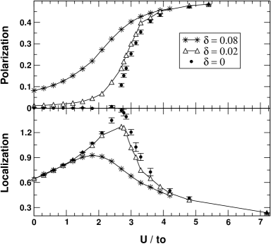
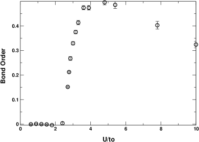
The phase transition we observe using QMC differs from the topological transition found using exact diagonalization and HF. As previously mentioned, in the BI and MI phases the polarization is restricted to or . Resta and Sorella identified the shift from to as the signature of a transition. However, we observe that takes a continuous range of values in the centrosymmetric limit which cannot occur in either the BI or the MI phase. This can only occur if the global inversion symmetry of the lattice is broken by a long range bond ordered state, predicted by Fabrizio et al [25] on the basis of field theory arguments in which he mapped the Hamiltonian onto two Ising spin models. The order parameter of this phase transition is the average bond order function , where is given in Eq 7. The spontaneous bond order of the centrosymmetric lattice is obtained by extrapolating to the of the same distorted lattices as before. We fixed the supercell size to sites and found the consequent size effects are within order of the error with which we can measure the bond order. These results are plotted in Fig 7.
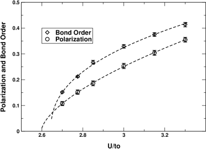
We have attempted to classify the quantum phase transition by fitting the polarization and bond order of the centrosymmetric lattice to a function of the form
| (36) |
where is the critical exponent and determines the universality class of the transition. A non-linear least squares routine was used to fit the data, with fitted parameters , , and listed in Table I. In Fig 8 the data for and and the corresponding fits are plotted. Both quantities behave similarly near the critical point and the of each is nearly identical. We find for and are near , the expected mean field exponent. On the other hand, Fabrizio, et al.[25], predicted that the transition is of the Ising universality class and thus should be . We do not know whether the difference is real or it is simply due to the possibility that the range of over which the scaling belongs to the universality class is too small for us to observe in the present work.
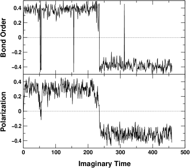
Alternatively, the existence of the bond ordered state can be observed by directly studying the symmetric lattice without any lattice distortion. Quantum Phase transitions (QPT) are characterized by a symmetry breaking that occurs in the thermodynamic limit. Below the lattice is a band insulator with no bond order but above the electrons will spontaneously choose to bond order with . There are two such states characterized by the same magnitude but opposite sign of the bond order. For any finite system the ground state remains a linear combination of both. However in the limit one of these is arbitrarily chosen as the ground state. Even though the QMC simulations of the symmetric lattice for measure zero bond order and polarization for long simulations, the imaginary time evolution of the simulations clearly depict the projected ground state moving from one of these bond ordered states to the other. This phase separation gives rise to large auto correlation times. The evolution of the bond order and polarization in imaginary time are illustrated in Fig 9 for and sites. As the ground state moves between BO states of opposite symmetry both the polarization and dimerization are observed to change sign. This provides an alternative method of detecting the existence of the BO state.
At large one might expect that the ionic Hubbard model is a Mott Insulator. Fabrizio, et al.[25], predict the existence of a Kosterlitz-Thouless transition for large at which the lattice becomes a Mott Insulator. Such a transition would be characterized by polarization of and no bond order. On the contrary we do not observe either for any considered which included values up to . The bond order does diminish but appears to asymptotically approach and the polarization appears to converge to only in the limit of . Yet working with such strongly correlated systems has the disadvantages that (i) fluctuations of the local estimators increase due to greater inaccuracies in the trial wavefunction and (ii) forward walking works so long as the trial wavefunction has some overlap with the exact ground state and as U increases overlap with the exact ground state diminishes.
C Phase transition as a function of ionicity
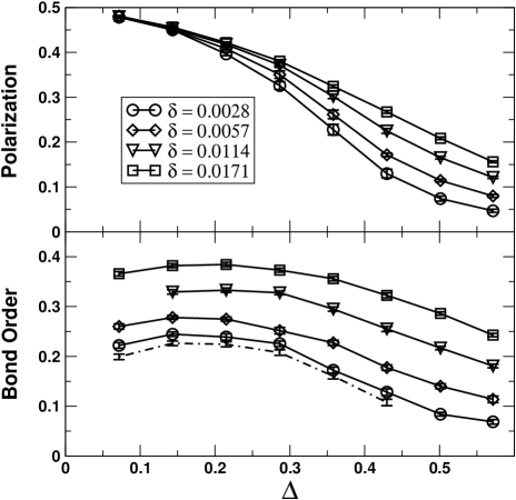
An alternative approach to study the phase transition(s) is to diminish the ionic potential while keeping fixed, so that the ratio increases. We have fixed the strength of electron correlation to and studied the bond order and polarization for . The behavior of the centrosymmetric lattice is inferred using two approaches (i) extrapolating results obtained on lattices with and (ii) looking for evidence of phase separation in the symmetric case. Fig 10 shows the results of the first approach for a fixed supercell length of sites. In the first we’ve neglected size effects and fixed the super cell length to sites. At large the single body contribution to the Hamiltonian is the dominant term and the lattice is a band insulator. Consequently the bond order and polarization are . However, as a transition occurs to a BO state where the bond order is non-zero and the polarization assumes values between and as before. (The transition is rounded at this fixed cell length.) The bond order in the limit is shown by the dotted line in Fig 10. These results were obtained by linearly extrapolating the bond order at finite . (No extrapolation was performed for the polarization since it is sensitive to size effects that were addressed in the previous section.)
Our results indicate the bond-order state exists at all values of studied. The finite value of the bond order for shown in Fig 10 contrasts sharply with the vanishing of the bond order as for the non-ionic Hubbard model () as shown in Fig 2. At , we always find and polarization equal 1/2 as they must be for a MI state with no long range order. However, our QMC simulations of the symmetric case ( and ) at the smallest value of the ionic potential studied reveal two BO states phase separating in imaginary time qualitatively the same as shown in Fig 9. Thus from our studies, there is no sign of a second transition to a MI state as proposed by Fabrizio, et al.[25], and the long range bond ordered state in Fig 10 appears to exist for any finite .
This implies that the MI state in exists only within the usual Hubbard model and in ionic Hubbard lattices only in the limit . At large the ionic Hubbard model has been mapped onto the Heisenberg spin model. The present finding suggests that such a mapping may be insufficient for Hubbard models with ionic potentials and that terms ignored or considered small possibly play a fundamental role.
VI Long Range Order as Inferred by Bond Order Correlation Function
Existence of a long range bond ordered state can be inferred by measuring the bond order correlation function (). We define as
| (37) |
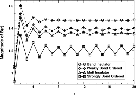
where is defined in Eq. 7 and is the strength of the bond of the lattice. If the BO state exists then this correlation function would be staggered as a consequence of the periodic arrangement of dominant and weak bonds. In Fig. 11 is plotted for separate cases: (i) , , (ii) , , (iii) , , and (iv) , , . The first case corresponds to the band insulating regime in which exponentially approaches a constant, confirming the lack of any long range ordered phase. Conversely in the last case, which corresponds to the system in Fig 9 that exhibited phase separation, its clearly visible that is staggered, signifying the presence of a long range bond ordered state. Finite size effects in each of these cases were determined to be miniscule and small systems were deemed sufficient to measure . The second case corresponds to diminishing so as to move the system towards the established Mott State of the usual Hubbard model. At this point in the phase diagram the wells of the bimodal distribution are weakly defined; thus making it extremely difficult to observe the phase separation of the bond order parameter directly. In contrast, the bond order correlation function is clearly staggered, though to a lesser degree than that of the later case. Case iii) is the Mott state of the usual Hubbard model. The staggered behavior of does not approach a finite limit at large , but rather tends to in a fashion that appears to be a power law ; contrary to the exponential convergence observed in the BI regime. Comparison of cases ii) and iii) shows that in each case the staggered behavior of is longer ranged than in the band insulating and strongly bond ordered cases; this exemplifies the difficulty of measuring the bond order or the phase separation of this generalized model as the ionic potential tends to zero.
The staggered nature of can be used to determine the mean bond order of the lattice. Defining two new variables
| (38) |
and
| (39) |
and substituting Eq 37 in place of we can relate these two quantities in terms of measurable quantities. At large the and bonds are uncorrelated and is the RMS bond order of the lattice whereas is the square of the average bond strength.
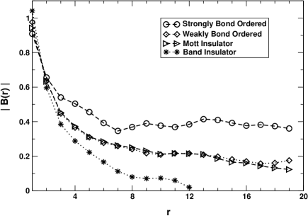
In the limit of large the average bond order can be expressed in terms of as:
| (40) |
This estimate is exact when where is the correlation length. Fig 12 shows plotted vs r for the same cases as in Fig 11. The strongly bond ordered system converges to an estimate of the bond order that is remarkably close to that obtained by extrapolating from distorted lattices (). The weakly bond ordered case appears to converge to a value near which is in reasonable agreement with the extrapolated value of . The band insulating estimate rapidly approaches as a function of , whereas the Mott insulating system appears to approach in a power law fashion.
VII Discussion
One of the primary results of the present work is the quantitative demonstration of the stability of the bond-ordered phase for interaction above a critical value for any non-zero . Most of our work was carried out through dimerizing the lattice by and examining the limit. There were two reasons for this: (i) this is an aid in the actual calculations which are stabilized by the applied bias, and (ii) the variation with dimerization is important in and of itself. Regarding the second point, it is well known that the ordinary non-ionic Hubbard model is unstable to dimerization, with a logarithmic Peierls instability at that becomes a stronger fractional power law instability at large [31, 32, 33, 34, 51, 52]. Our work shows that as a function of the ionic Hubbard model undergoes a phase transition from a stable non-dimerized BI phase to a correlated phase in which the instability is more severe than in the non-ionic Hubbard model. This is evident in comparison of Fig.2 with Figs. 5 and 7. In the former for the non-ionic case, the decrease of the bond order with is clearly observed and is consistent with previous theoretical predictions of the power law form. However, in all the calculations for the ionic model for above the critical value, the average bond order is found to extrapolate to a non-zero value. This is observed even for much smaller than previous studies. From this evidence alone there are two possibilities: 1) the BO phase with broken symmetry is stable at zero dimerization, or 2) there is non-analytic behavior as which is even stronger than that for the non-ionic Hubbard model.
This result is sufficient to draw conclusions about real 1D systems in which the sites are allowed to dimerize if this leads to lower energy. In either scenario above dimerization would always occur (except in the BI phase). In the former case the BO phase would occur spontaneously and by symmetry there would always be an accompanying lattice distortion. In the second scenario, dimerization would occur and lead to bond order. The symmetric Mott insulator would never occur and the only transition would be from a BI phase to a dimerized BO phase.
At this point we can compare with experiment on 1D materials. Experimental works by Torrance, et al.,[56] observed a second order transitions between neutral (BI) and ionic (BO) states in organic charge transfer solids. The transition occurs upon applying pressure over a wide range of temperatures and was attributed to the rise in Madelung energy of the crystal. No state synonymous to the Mott state was observed.
In addition, however, calculations on the centrosymmetric lattice show directly existence of the BO phase in our simulations. One observation is the “phase separation” or “flip-flop’ between left and right BO phases as a function of imaginary time in the QMC simulations. The other is the staggered behavior of the BO correlation functions for which the numerical data out to large distance supports power law behavior in the non-ionic case and long range order in the ionic case.
Other work on related systems also has identified BO phases. Recent work by Nakamura [26] in the extended Hubbard model has found a rich phase diagram in which there are transitions from a and regime. The extended Hubbard model differs from the ionic model studied here in that there is an additional next nearest neighbor coulomb potential and no ionic potential . Nakamura identifies the first transition as belonging to the gaussian universality class and the later as a Kosterlitz-Thouless transition. The phase observed by Nakamura exists at all down to the usual Hubbard model (); where both the gaussian and the KT transitions coexist. We can imagine the at which the transition takes place increasing concurrently as the ionic potential is increased from zero.
Let us now consider why the BO phase was not found in previous studies that used exact diagonalization Lanczos techniques to treat small finite systems[13, 53]. There are two reasons why these studies did not find the BO phase. In the BO phase the energy can parameterized by the bond order parameter (Eq 7) that develops a bimodal distribution with minima at . The true ground state is a linear combination of these degenerate BO states,
| (41) |
which of course has no net bond order. The situation is similar in many aspects to a ferromagnet; it is only in the thermodynamic limit that one or the other of the two states is the true ground state with long range order. For finite systems existence of the BO state can be inferred from correlation functions; however, to our knowledge this has not been done in other work.
A second reason that the BO states have not been observed may be that there is no bimodal distribution for the small cells studied by exact diagonalization. We have addressed this issue using QMC by measuring the average bond order on distorted lattices of sites and extrapolating to the centrosymmetric limit. At this point in the phase diagram (, ) lattices with less than sites do not exhibit the BO phase and only upon working with larger supercells does QMC detect the phase separation of the two BO states. Consequently, exact diagonalization methods are not currently feasible in such cases since they scale exponentially with .
Recent work using the density matrix renormalization group (DMRG) method has reported results for charge and spin gaps in these models. This approach should enable one to distinguish the phases since (i) in the BI phase, (ii) in the BO phase, and (iii) but in the MI phase. It was found to be very difficult and to require extremely large cells to determine spin gaps in the BO/MI phases, and the two reports came to opposite conclusions on the existence of the BO phase. In our QMC calculations we have also determined the charge and spin gaps. Our estimates of the charge gap are in qualitative agreement with other works; however, the spin gap is very small in all cases except in the BI regime and statistical noise does not permit accurate determination of such small gaps in QMC.
Both DMRG calculations find the spin gap to vanish, i.e., the MI phase to be the ground state for large . We have no direct explanation of this difference: it may be that our procedure is not sufficiently accurate to determine the BO-MI transition, which is the most difficult part of the present work. On the other hand, it may be that the DMRG calculations on finite cells with open boundary conditions may have difficulties: the surface effects break the symmetry of the problem which may lead to extremely problematic size effects and potential errors. In any case, we are very confident that our work establishes that the BO state is either the ground state or very close to the ground state in energy; this is clear from our tests on the ordinary Hubbard model shown in Fig. .
VIII Conclusions
We have studied the phase diagram of an idealized dielectric, the D ionic Hubbard model proposed by Nagosa[23] and Egami[24]. This model undergoes a phase transition as a function of the on-site interaction , which has been a source of controversy. The only previous quantitative studies[13, 53] concluded that at a critical there is an abrupt ”topological” transition from a band insulator to a Mott insulator with no broken symmetry or long range order in either phase. The signature of the transition was found to be an abrupt change of in the polarization at which the effective charge diverged signifying the delocalization of the electron states[13, 53]. Recently, however, there has been a prediction[25] that this model would exhibit two quantum phase transitions: the first signifying a change of state from a band insulator to a broken symmetry phase with long range alternating bond order, and the second a transition to the Mott insulator.
We have studied this model using quantum Monte Carlo methods which allow the simulation of much larger systems than studied by exact diagonalization[13, 53]. To our knowledge, this is the first application of QMC to determine the polarization and localization of an electronic system. We evaluate the expectation values of the bond-order, polarization and localization using the expressions Eqs 7, 10 and 11. It is found that upon crossing a critical value a change of phase occurs from a band insulating to bond-ordered state. The bond order develops continuously (See Fig 8) as a function of and since the inversion symmetry is broken, the polarization also varies continuously, unlike the results of the small cell exact-diagonalization calculations.[13] The critical behavior is uniquely determined by fitting the bond order and polarization to a scaling function near the critical regime. We find an exponent near 1/2, which differs from that for the Ising class proposed in Ref [25]; however, it may be that we are outside of the regime in which the scaling belongs to the appropriate universality class. In addition, we found that there is a metallic point at where the system is metallic. At this point the charge gap must vanish which we have found in pure ground state calculations by determining the fluctuations of the polarization. The calculations determine quantitatively the localization length[13, 14, 15], which diverges at the transition.
An important part of the present QMC work is that we use a forward projection scheme which allows exact estimates, in principle, of any operator, including ones such as the polarization (or center of mass position operator) that do not commute with the Hamiltonian. Furthermore the nodes of this D model are known exactly, so the QMC method is in principle exact. In order to confirm the existence of the bond ordered state, we carried out calculations on dimerized lattices () whose inversion symmetry is explicitly broken, and let become small. QMC allows us to work with large enough lattices so as to study systems with levels of dimerization much smaller than previously feasible[31, 32, 33, 34, 51]. We find good agreement with previous results obtained from the Heisenberg spin model that predict electronic correlation enhances the instability to bond ordering.[52, 51] In addition, we can see from the simulations of the symmetric lattice that the system is alternating between the two degenerate states of bond-order (see Fig 9).
We have searched for the proposed transition to a Mott insulating state, but we have not observed such a transition from the bond ordered regime even for very large or very small . Even the smallest value of considered in this study () is sufficient to cause the ionic Hubbard model to be unstable to bond ordering, although there is no broken symmetry in the usual Hubbard model (), neither in the exact solution[22] nor in our results. Thus our results show that the instability to dimerization is even stronger in the ionic model than that known previously for the ordinary non-ionic Hubbard model.[31, 32, 33, 34, 51, 52]. Furthermore, for the centrosymmetric lattice (), calculations of correlation functions and observations of “flip-flop” between left and right bond-ordered states in the QMC simulations provides further evidence for the stability of the bond-ordered state.
Among the interesting consequences of the stability of the BO state is the existence of fractional charges.[57, 25] For the case of a dimerized or bond-ordered state, the charge is an irrational fraction the value of which depends upon the value of [57, 25].
Finally, these results imply that if dimerization is allowed (which is always the case in real materials since the atoms can always dimerize if it lowers the energy) then the symmetric Mott state is never stable and the only phase transition is from the symmetric BI to the dimerized BO state. This is experimentally confirmed by Torrance et al.[56]; where upon increasing the electronic interaction a transition takes place.
IX Acknowledgements
We gratefully acknowledge Erik Koch for his help implementing lattice quantum Monte Carlo methods and David Campbell, Michele Fabrizio, Eduardo Fradkin, Erik Koch, Gerardo Ortiz, Rafaelle Resta, Anders Sandvik, Pinaki Sengupta, Ivo Souza and David Vanderbilt for invaluable discussions. This work would not have been feasible without the computational resources of the National Supercomputing Center at the University of Illinois and the Materials Research Laboratory. We are especially grateful to the NT supercluster, managed by Rob Pennington and Michael Showerman, which provided the majority of the computational resources for this study. This work was supported by the National Science Foundation Grant No. DMR .
| A | |||
|---|---|---|---|
| 0.44(1) | 2.60(5) | 0.60(10) | |
| 0.49(1) | 2.65(2) | 0.39(4) |
REFERENCES
- [1] M. Imada, A. Fujimori and Y. Tokura, Rev. Mod. Phys. 70, 1039 (1998) and references therein
- [2] N. F. Mott, Proc. R. Soc. London A 382, 1 (1982)
- [3] N. F. Mott, Proc. Phys. Soc. A 62, 416 (1949)
- [4] J. C. Slater, Phys. Rev. 82, 538 (1951)
- [5] D.H. Lee and R. Shankar, Phys. Rev. Lett. 65, 1490 (1990)
- [6] D. J. Griffiths, . Prentice-Hall Inc., New Jersey, 1989.
- [7] L.D. Landau, E.M. Lifshitz, Electrodynamics of Continuous Media, Pergamon Press, Oxford, England (1988)
- [8] W. Kohn, Phys. Rev. 133, A171 (1964)
- [9] R. D. King-Smith and D. Vanderbilt, Phys. Rev. B. 47, 1651 (1993)
- [10] G. Ortiz and R. M. Martin, Phys. Rev. B 49, 14202 (1994)
- [11] R. Resta, Phys. Rev. Lett. 80, 1800 (1998)
- [12] R. Resta, S. Sorella, Phys. Rev. Lett. 82, 370 (1999)
- [13] R. Resta, S. Sorella, Phys. Rev. Lett. 74, 4738 (1995)
- [14] A. A. Aligia, G. Ortiz , Phys. Rev. Lett. 82, 2560 (1999)
- [15] I. Souza, T. Wilkens and R.M. Martin, to be published in Phys. Rev. B. (2000)
- [16] M. V. Berry, Proc. R. Soc. London, Ser. A 392, 45 (1984)
- [17] C. Gros, Z. Phys. B 86, 359 (1992)
- [18] D. J. Scalapino, S. R. White and S. Zhang, Phys. Rev. B 47, 7995 (1993)
- [19] N. Beyers and C. N. Yang, Phys. Rev. Lett. 7, 46 (1961)
- [20] Hubbard J, 1963, A 276, 238
- [21] J.M.P. Carmelo, F.Guinea and E.Louis, . Plenum Press, New York, 1995
- [22] E. H. Lieb and F. Y. Wu, Phys. Rev. Lett. 25, 1445 (1968)
- [23] N. Nagaosa and J. Takimoto, J. Phys. Soc. Jpn. 55, 2735 (1986)
- [24] T. Egami, S. Ishihara, and M. Tachiki, Science 261, 1307 (1993)
- [25] Michele Fabrizio, Alexander O. Gogolin, and Alexander A. Nersesyan, PRL 83, 2014 (1999)
- [26] Masaaki Nakamura, Phys. Rev. B 61, 16377 (2000)
- [27] Yasutami Takada, Manabu Kido, condmat/0001239
- [28] S. Qin, J. Lou, T. Xiang, Z. Su, G. Tian, condmat/0004162
- [29] W. M. C. Foulkes, L. Mitas, R. J. Needs and G. Rajagopal, to be published in RMP
- [30] I.I. Ukrainskiĭ, Sov. Phys. JETP 49, 381 (1979)
- [31] D. Baeriswyl and K. Maki, Phys. Rev. B 31, 6633 (1985)
- [32] G. W. Hayden and Z. G. Soos, Phys. Rev. B 38, 6075 (1988)
- [33] P. Horsch, Phys. Rev. B 24, 7351 (1981)
- [34] J. E. Hirsh, Phys. Rev. Lett. 51, 296 (1983)
- [35] W. P. Su, J. R. Schrieffer, and A. J. Heeger, Phys. Rev. Lett. 42, 1698 ( 1979)
- [36] Charles Kittel, Introduction to Solid State Physics John Wiley and Sons, New York (1986)
- [37] C. A. Coulson, Proc. R. Soc. London, Ser. A bf 169, 413 (1939)
- [38] Eduardo Fradkin, Field Theories of Condensed Matter Systems Addison-Wesley Publishing Company, New York (1991)
- [39] R. M. Martin and G. Ortiz, Solid State Comm. 102, 121 (1997).
- [40] R. Resta, RMP 66, 899 (1994)
- [41] N. Marzari and D. Vanderbilt, Phys. Rev. B, 56, 12847 (1997)
- [42] F. Bolton, Phys. Rev. B. 54, 4780 (1996)
- [43] G. Ortiz, D. M. Ceperley, and R. M. Martin, Phys. Rev. Lett. 71, 2777 (1993)
- [44] B. L. Hammond, W. A. Lester, P. J. Reynolds, Monte Carlo Methods in Ab Initio Quantum Chemistry World Scientific, New Jersey (1994)
- [45] N. Metropolis, A.W. Rosenbluth, M.N. Rosenbluth, A.M. Teller and E. Teller, Journal of Chem. Phys. 21, 1087 (1953)
- [46] Gutzwiller, M. C., 1963, Phys. Rev. Lett. 10, 159
- [47] Guozhong An and J. M. J. van Leeuwen, Phys. Rev. B, 44, 9410 (1991)
- [48] Koonin, Steven E. and Meredith, Dawn C., . Addison-Wesley Publishing Company, Canada, 1990
- [49] D.F.B. ten Haaf , Phys. Rev. B 51, 13039 (1995)
- [50] K. Hashimoto, Int. J. Quantum Chem. 28, 581 (1985)
- [51] Z. G. Soos, S. Kuwajima, and J. E. Mihalick, Phys. Rev. B 32 3124 (1985)
- [52] J. L. Black and V. J. Emery, Phys. Rev. B 23, 429 (1981)
- [53] G. Ortiz, P. Ordejn, R. M. Martin, G. Chiappe, Phys. Rev. B 54, 13515 (1996)
- [54] N. Gidopoulos, S. Sorella and E. Tosatti, condmat/9905418
- [55] Erik Koch, Olle Gunnarsson, and Richard M. Martin, PRB 59, 15632 (1999)
- [56] J. B. Torrance ., 1981, Phys. Rev. Lett. 47, 1747
- [57] M. J. Rice and E. J. Mele, 1982, Phys. Rev. Lett. 49, 1455