Stochastic Penna model for biological aging

Abstract

A stochastic genetic model for biological aging is introduced bridging the gap between the bit-string Penna model and the Pletcher-Neuhauser approach. The phenomenon of exponentially increasing mortality function at intermediate ages and its deceleration at advanced ages is reproduced for both the evolutionary steady-state population and the genetically homogeneous individuals.
Keywords: Biological Aging; Mortality; Penna Model.

1 Introduction

The problem of biological aging has attracted much attention in recent years. Based on the data of human demography and experiments of other living organisms, many important phenomena of longevity have been found [1, 2, 3]. For instance, the Gompertz law was observed for intermediate ages, that is, the mortality function increases exponentially with age, while at old ages the mortality was found to decelerate or level off, and even decline for some organisms like flies, worms, and yeast [2, 4, 5].

To reproduce and explain these phenomena, various models of senescence have been proposed, with genetic or nongenetic mechanisms [1, 2, 3, 6, 7]. Among them, the one widely used by physicists is the Penna model [7, 1], where one computer word is used to represent the inherited genome of one individual and each bit of the word corresponds to one age of the individual lifetime. A bit set to one represents a deleterious mutation and the suffering from an inherited disease from this age on, and the individual will die if the accumulation of these set bits exceeds a threshold.

Although the Penna model has been well applied to many problems related to biological aging [1, 8], there exists an important flaw in this model as pointed out by Pletcher and Neuhauser very recently [3]. That is, the model predicts that for a genetically identical population all individuals have their genetic death at the same age, but this is inconsistent with the experimental results [4, 2] which also exhibited the exponential Gompertz law and the deceleration of the old age mortality for the genetically homogeneous case. Thus, a more complicated model has been proposed [3].

In this paper we develop a simpler stochastic model bridging the gap between the standard (deterministic) Penna model and the Pletcher-Neuhauser approach. The simulations and analytic results of this model are shown to agree with some features of the biological aging, e.g., the exponential increase of the mortality function and the deceleration at advanced ages, and the flaw of the Penna model mentioned above can be avoided.

2 Model

As in the standard Penna model, here the genome of each individual is characterized by a string (computer word) of 32 bits, and each bit is expressed as a particular age in the life of the individual. A bit $i$ is set to $1$ if it represents a deleterious mutation, and from this age $i$ on this bit will continuously affect the survival probability of the individual. That is, at age $a$ ($\geq i$) the death probability contributed by the mutated bit $i$ is $f(a-i)$, with the corresponding survival probability $1-f(a-i)$. Otherwise, this bit is set to zero and has no effect on death. Thus our assumptions are very different from an earlier ”Fermi” function in another stochastic Penna model [9].

The individual’s survival probability $G$ up to age $a$ is the product of the contributions from all the bits before $a$:

$$G(1,2,...,a)=(1-b_{1}f(a-1))(1-b_{2}f(a-2))\cdots(1-b_{i}f(a-i))\cdots(1-b_{a}f(0)),$$ (1)

where $b_{i}=1$ or $0$ ($i=1,...,a$) represents the $i$th bit. With the form of $f(a-i)$, one can obtain the mortality function by simulation or analytical work. In this work we simply assume that

$$f(a-i)=(a-i+1)C,$$ (2)

with the constant $C=0.03$ and the limit $f\leq 1.0$, which means that the contribution of death probability from bit $i$ (if set to $1$) is assumed to increase linearly with the age. The other forms of $f(a-i)$, such as the exponential and the square root forms, have been tried, and we have also simulated the other probabilistic Penna model with Fermi function [9]. Although some phenomena for the genetically heterogeneous steady-state population can be reproduced, they cannot give a good result for the genetically homogeneous populations.

The alive individual will generate $B$ offsprings from the minimum reproduction age $R_{\rm min}$ to the maximum one $R_{\rm max}$, and the genome of each offspring is the same as the parent one, except for $M$ mutations randomly occurring at birth. At each time step $t$, a Verhulst factor $V=1-N(t)/N_{\rm max}$ denoting the survival probability of the individual due to the space and food restrictions is introduced, where $N(t)$ is the current population size and $N_{\rm max}$ is the carrying capacity of the environment, usually set to $10N(0)$. In the next section 3 the simulations based on these rules are presented, while for genetically identical individuals, which have the same genotype randomly sampled from the simulated steady-state population, the analytic results can be derived, as shown in section 4.

Moreover, in this paper the mortality function $\mu(a)$ at age $a$ is defined as

$$\mu(a)=-{\frac{d\ln N_{a}}{da}}\simeq-\ln S(a),$$

where $N_{a}$ denotes the number of alive individuals with age $a$, and $S(a)=N_{a+1}/N_{a}$ is the survival rate. To eliminate the effect of the Verhulst factor, the normalized mortality function is preferred [1], i.e.,

$$\mu(a)=-\ln[S(a)/S(0)].$$ (3)

3 Simulations

In our simulations, initially the population size $N(0)$ is $10^{7}$ and all bits of all the strings are set to zero, i.e., free of mutations. One time step $t$ corresponds to one aging interval of the individuals, or reading one bit of all strings. The reproduction range is set from $R_{\rm min}=6$ to $R_{\rm max}=20$ with the birth rate $B=1$, and the results are similar if using the maximum value of $R_{\rm max}=32$. $M=1$ mutation for each offspring genome is introduced at birth, and here only the bad mutations are taken into account, that is, the bit randomly selected for mutation is always set to $1$. (The good mutations have also been considered, e.g., 10% good mutations and 90% bad ones, and similar results are found.)

Fig. 1 shows the evolution of the whole population size $N(t)$ until $t=10^{4}$. Similar to the standard Penna model, the steady-state population is obtained at late timesteps, and as a result of evolution and selection, the frequency of deleterious bits (set as $1$) for the individual of the steady-state population is low at early ages (especially before the reproduction age) and very high at old ones. This behavior of the frequency (or the bad mutation rate) is shown in the inset of Fig. 1.

The mortality function is calculated using Eq. (3) and averaged over the steady-state population from timesteps 5000 to 10000, as shown in Fig. 2. The result is consistent with the experimental and empirical observations [1, 2], that is, at intermediate ages the mortality function increases exponentially, exhibiting the Gompertz law, and deceleration occurs for old ages. For comparison, the mortality simulated by the standard (deterministic) Penna model is also shown in Fig. 2, with the threshold of the accumulated bad mutations $T=3$ and the other parameters unchanged. The exponential Gompertz law can also be obtained for the standard Penna model [1], however, no deceleration is observed except for suitable modifications summarized in [1]; see also [9].

4 Genetically identical population

To study the genetically homogeneous population, one can randomly sample an individual (genotype) from the simulated steady-state population, and then ”clone” it to create the whole genetically identical population. According to the form of these bit-strings, the mortality function can be derived and calculated analytically.

As in some experiments of fruit flies [4], reproduction is prevented during the aging of genetically homogeneous individuals. Thus, for this population of single genotype, we have

$$N_{1} =N_{0}(1-b_{1}f(0))=N_{0}G(0),$$

$$N_{2} =N_{1}(1-b_{1}f(1))(1-b_{2}f(0))=N_{1}G(1,2),$$

$$\vdots$$

$$N_{a} =N_{a-1}(1-b_{1}f(a-1))(1-b_{2}f(a-2))\cdots(1-b_{a}f(0))=N_{a-1}G(1,2,...,a),$$

$$\vdots$$

where $N_{a}$, $a=1,2,...,32$, is the number of individuals with age $a$ in the population, and the function $G(1,2,...,a)$ is defined by Eq. (1). Then the survival rate is easily obtained:

$$S(a)=\frac{N_{a+1}}{N_{a}}=G(1,2,...,a+1).$$ (4)

For the mortality function, the normalized formula (3) is used to be consistent with the simulations in Sec. 3, and then we have

$$\mu(a)=-\ln[G(1,2,...,a+1)/G(1)].$$ (5)

Different genotypes have been selected randomly from the stable population of Sec. 3, and the corresponding mortality function of each type is calculated using Eq. (5). Some examples are shown in Fig. 3 for linear-log plots, where part of them obey the exponential Gompertz law at the intermediate ages, similar to that of the above simulation (Sec. 3) and experiments [2, 4]. Moreover, all of these curves exhibit the deceleration for old ages.

Moreover, the analytic calculation is also available if the reproduction is allowed as in other experiments of genetically identical population, but for the case of no mutation. The details are shown in the appendix, and the mortality function derived is the same as Eq. (5).

5 Discussion and conclusion

In this paper a stochastic genetic model of aging is developed based on the bit-string asexual Penna model, and the results of the exponentially increasing mortality at intermediate ages and its deceleration at old ages are obtained for both the genetically heterogeneous steady-state population and the homogeneous individuals. However, the decrease of mortality for the oldest ages, observed in some experiments [2], cannot be described by the mechanism of this model.

Although the properties for intermediate and old ages have been well simulated in this model, the behavior at early ages cannot be well reproduced, which is also an artifact of the Penna-type genetic models. From Fig. 3 for genetically identical populations, it can be found that some populations have unrealistic zero mortality at some early ages. Thus, the effects for the early ages studied in the experiments, such as the investigations of genetic variation for ln-mortality contributed by steady-state population or by new mutations [10], cannot be produced in this model. More efforts should be made to avoid this difficulty, e.g., by considering different kinds of genes before and after the reproduction age [11].

Appendix

Here an example of the analytic solution for this stochastic model is presented, for the case where the reproduction is allowed in the aging process of genetically identical population, but no mutation occurs when generating the genomes of offsprings. Thus, the individuals keep homogeneous, characterized by the same bit-string $b_{1}b_{2}...b_{L}$ with $L$ the length of genome ($L=32$ in above studies).

When the system evolves to the steady state, the population size at timestep $t$ of this state

$$N(t)=N_{0}(t)+N_{1}(t)+\cdots+N_{L}(t)$$ (6)

as well as the Verhulst factor $V$ can be considered as constant. Thus, the numbers of individuals with ages from $1$ to $L$ at this step $t$ are

$$N_{L}(t)=N_{L-1}(t-1)VG(1,2,...,L),$$

$$N_{L-1}(t)=N_{L-2}(t-1)VG(1,2,...,L-1),$$

$$\mbox{}\hskip 28.45274pt\vdots$$

$$N_{a}(t)=N_{a-1}(t-1)VG(1,2,...,a),$$

$$\mbox{}\hskip 28.45274pt\vdots$$

$$N_{1}(t)=N_{0}(t-1)VG(1),$$ (7)

where $G(1,2,...,a)$ is the living probability of individual at age $a$, as defined in Eq. (1), and the individuals of age zero (newly born) are generated by the ones with reproducible age (from age $R_{\rm min}$ to $R_{\rm max}$), that is,

$$N_{0}(t) = B[N_{R_{\rm min}}+N_{R_{\rm min}+1}+\cdots+N_{R_{\rm max}}]$$ (8)

$$= BV[N_{R_{\rm min}-1}(t-1)G(1,2,...,R_{\rm min})+N_{R_{\rm min}}(t-1)G(1,2,...,R_{\rm min}+1)$$

$$+ \cdots+N_{R_{\rm max}-1}(t-1)G(1,2,...,R_{\rm max})]$$

with the birth rate $B$.

Consequently, the number of individuals with certain age $a$ ($0<a\leq L$) can be expressed as

$$N_{a}(t)=N_{0}(t-a)V^{a}G(1)G(1,2)\cdots G(1,2,...,a).$$ (9)

Therefore, if $N_{0}(t)$ is unchanged for the steady state, all the $N_{a}(t)$, $a=1,...,L$, will also keep unchanged, i.e., independent of timestep $t$, and then the survival rate $S$ can be obtained from Eq. (7), that is,

$$S(a)=N_{a+1}/N_{a}=VG(1,2,...,a+1)$$

and

$$S(0)=N_{1}/N_{0}=VG(1).$$

The Verhulst factor can be eliminated when calculating the normalized rate:

$$S(a)/S(0)=G(1,2,...a+1)/G(1),$$

and from the definition of Eq. (3) one can obtain the normalized mortality function, which is the same as Eq. (5).

The constant property of the population size $N(t)$ and the number $N_{0}(t)$ for age $0$, as well as the above analytic result of the mortality function have been confirmed by the simulation. Moreover, the steady state condition can be derived from Eqs. (8) and (9), which is

$$BV^{R_{\rm min}}G(1)G(1,2)\cdots G(1,2,...,R_{\rm min})[1+VG(1,2,...,R_{\rm min}+1)$$

$$+V^{2}G(1,2,...,R_{\rm min}+1)G(1,2,...,R_{\rm min}+2)+\cdots$$

$$+V^{R_{\rm max}-R_{\rm min}}G(1,2,...,R_{\rm min}+1)\cdots G(1,2,...,R_{\rm max})]=1,$$ (10)

depending on the parameters $B$, $R_{\rm min}$, and $R_{\rm max}$.

Figure 1: The evolution of the whole population size $N(t)$ with time step $t$, for the initial population $N(0)=10^{7}$ and the parameters $R_{\rm min}=6$, $R_{\rm max}=20$, $B=1$, and $M=1$. Only the bad mutations are considered. Inset: the frequency of deleterious bits (set as $1$) as a function of age for the individuals of the steady-state population (averaged over timestep 5000 to 10000).

Figure 2: Linear-log plot of the mortality function for the evolutionary steady-state population, with the same parameters of Fig. 1 and averaged over timestep 5000 to 10000. The mortality of the standard (deterministic) Penna model is also shown (pluses) for comparison, with the same parameters as well as the death threshold $T=3$.

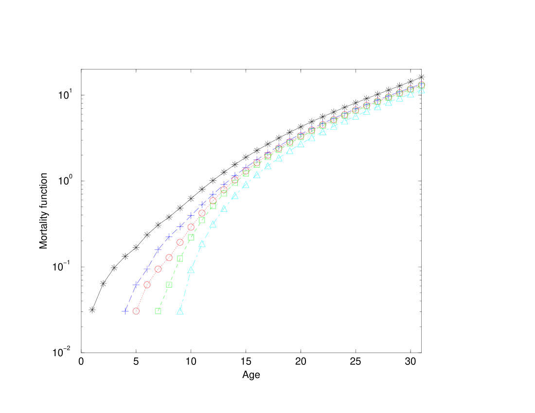
Figure 3: The mortality function for the genetically identical populations, with each genotype randomly sampled from the steady-state population of the simulation shown in Figs. 1 and 2. The results are calculated by Eq. (5), and shown in the linear-log plots.

References

- [1] S. Moss de Oliveira, P. M. C. de Oliveira, and D. Stauffer, Evolution, Money, War and Computers (Teubner, Stuttgart-Leipzig, 1999).
- [2] J. W. Vaupel, J. R. Carey, K. Christensen, T. E. Johnson, A. I. Yashin, N. V. Holm, I. A. Iachine, V. Kannisto, A. A. Khazaeli, P. Liedo, V. D. Longo, Y. Zeng, K. G. Manton, and J. W. Curtsinger, Science 280, 855 (1998).
- [3] S. D. Pletcher and C. Neuhauser, Int. J. Mod. Phys. C 11, 525 (2000).
- [4] J. W. Curtsinger, H. H. Fukui, D. R. Townsend, and J. W. Vaupel, Science 258, 461 (1992).
- [5] T. T. Perls, E. Bubrick, C.G. Wager, J. Vijg, L. Kruglyak, Lancet 351, 1560 (1998); P. M. C. de Oliveira, S. Moss de Oliveira, A. T. Bernardes and D. Stauffer, Lancet 352, 911 (1998).
- [6] J. W. Vaupel and J. R. Carey, Science 260, 1667 (1993).
- [7] T. J. P. Penna, J. Stat. Phys. 78, 1629 (1995).
- [8] T. J. P. Penna, S. Moss de Oliveira, and D. Stauffer, Phys. Rev. E 52, R3309 (1995); T. J. P. Penna and S. Moss de Oliveira, J. Physique I 5, 1697 (1995).
- [9] J. Thoms, P. Donahue, and N. Jan, J. Physique I 5, 935 (1995); J. Thoms, P. Donahue, D. L. Hunter, and N. Jan, ibid. 5, 1689 (1995); D. Stauffer, Int. J. Mod. Phys. C 10, 1363 (1999).
- [10] S. D. Pletcher, D. Houle, and J. W. Curtsinger, Genetics 148, 287 (1998); ibid. 153, 813 (1999).
- [11] E. Niewczas, A. Kurdziel, and S. Cebrat, Int. J. Mod. Phys. C 11, No. 4 (2000).