Hydrogen-Bonded Liquids: Effects of Correlations of Orientational Degrees of Freedom

Abstract

We improve a lattice model of water introduced by Sastry, Debenedetti, Sciortino, and Stanley to give insight on experimental thermodynamic anomalies in supercooled phase, taking into account the correlations between intra-molecular orientational degrees of freedom. The original Sastry et al. model including energetic, entropic and volumic effect of the orientation-dependent hydrogen bonds (HBs), captures qualitatively the experimental water behavior, but it ignores the geometrical correlation between HBs. Our mean-field calculation shows that adding these correlations gives a more water-like phase diagram than previously shown, with the appearance of a solid phase and first-order liquid-solid and gas-solid phase transitions. Further investigation is necessary to be able to use this model to characterize the thermodynamic properties of the supercooled region.

Introduction

Water has a temperature density maximum at 4 ^oC at ambient pressure, above the melting line. This is perhaps the most well-known anomaly of the many observed in liquid water. In the metastable, supercooled region of water, the anomalies are especially pronounced. The absolute magnitude of thermodynamic response functions such as isothermal compressibility Speedy76 , thermal expansion coefficient Hare86 , and isobaric heat capacity Angell82 are all known to increase dramatically as the temperature is lowered. The quest for an explanation has led to extensive experimental, numerical, and theoretical investigations of the properties of supercooled water AngellChapter ; BellissentBook ; Bellissent95 ; Mishima98 ; Smith99 ; Shiratani98 ; DebenedettiBook ; Ponyatovsky95 ; Roberts96a ; Roberts96b ; Reza98 However, in spite of many studies, a final answer has yet to be reached.

Three major theories have emerged from existing evidence. They are known as the stability-limit conjecture Speedy82 , the two critical-point modelPoole92 , and the singularity-free scenario Stanley80 ; Sastry96 ; Rebelo98 (Fig. 1). $i)$ The stability-limit conjecture assumes that the superheated liquid-to-gas spinodal and the supercooled liquid-to-solid spinodal in the pressure-temperature ($P,T$) phase diagram are connected at negative $P$. $ii)$ The two critical-point scenario does not assume such a retracing spinodal. Instead, it attributes the anomalies of water to a second critical-point in the supercooled region of the phase diagram. This critical-point comes at the end of a phase-transition line that separates two metastable liquid phases, a low-density liquid (LDL), and a high-density liquid (HDL). $iii)$ The singularity-free scenario does not attribute the anomalies in water to a transition in the supercooled region or a retracing spinodal, but to a line of temperatures of maximum density (TMD) in the stable liquid phase and in the super-heated liquid phase with positive $(\partial P/\partial T)_{TMD}$ (slope) in the $P,T$ plane at high $P$ and negative slope at lower $P$ (retracing TMD). The aforementioned response functions are not considered to diverge, but merely to have maxima. Note that even in the two critical points scenario the TMD is retracing. There are theoretical calculations that show that the apparent gap between these different scenarios can be reconciled without inconsistencies Poole94 ; Borick95 ; Roberts96b . Thus, the differences between the different scenarios may be much more subtle than expected. Authoritative experiments have not been forthcoming due to the difficulty of probing metastable water without encountering inevitable crystallization Mishima98 .

Figure 1: Three interpretations of the supercooled water phase diagram: a) stability limit conjecture, b) two critical-points model, c) singularity-free scenario. A dashed line denotes a spinodal, a bold line denotes a transition line, and a dotted line denotes a TMD line. The solid-liquid transition line is not shown; $C$ is the known critical point; $C^{\prime}$ is the hypothetical second critical point.

It is worth noting that these so-called anomalies are not unique to water. Although water exhibits anomalous properties relative to the liquid norm, namely argon-like liquids, its unusual characteristics are shared by other fluids such as $SiO_{2}$Grims84 and $GeO_{2}$Smith95 . What differentiates these anomalous liquids from normal liquids is that they form bonded networks that are dependent on the relative orientation of the molecules.

The effect of orientation-dependent, hydrogen-bonded networks on critical behavior has already been recognized. However, the effect of the intra-molecular correlation between the orientational degrees of freedom has not be explored thoroughly. For example, an open problem is how the intensity of orientational correlations can change the phase diagram. This is where our focus lies.

The Model

Our Hamiltonian can be expressed as:

$${\cal H}=-\epsilon\sum_{<i,j>}{n_{i}n_{j}}-\mu\sum_{i}n_{i}-\it{J}\sum_{<i,j>}{n_{i}n_{j}\delta_{\sigma_{ij}\sigma_{ji}}}-\it{J_{\sigma}}\sum_{i}n_{i}\sum_{(k,l)_{i}}{\delta_{\sigma_{ik}\sigma_{il}}}\ .$$ (1)

The first three terms constitute the original Hamiltonian Sastry96 ; Rebelo98 . The first two terms in the Hamiltonian are the standard lattice gas Hamiltonian where $n_{i}=0,1$ indicates whether site $i$ is occupied by a molecule, $\epsilon$ is the attractive energy between molecules, $\mu$ is the chemical potential and the symbol $\sum_{<i,j>}$ means that the sum is on all nearest neighbor (NN) lattice sites.

The third term in Eq.(1) describes the interaction of orientational degrees of freedom (arms) between neighboring molecules, and accounts for hydrogen bonding within the system. It is introduced in the following way: Each molecule has a maximum of $\gamma$ neighbors; Therefore, it has $\gamma$ arms that can potentially form HBs with the respective arms of its neighbors. Each of the arms can assume $q$ orientational states, so the total number of orientational states for a molecule is $q^{\gamma}$. The Potts variable $\sigma_{ij}=1,2,\ldots,q$ Potts specifies the orientational state of the arm of molecule $i$ that points toward nearest-neighbor molecule $j$. When two neighboring sites are occupied ($n_{i}=n_{j}=1$) and the orientational states of the two reciprocally pointing arms match ($\sigma_{ij}=\sigma_{ji}$), a HB forms ($\delta_{\sigma_{ij}\sigma{ji}}=1$ where $\delta_{ab}=1$ if $a=b$, otherwise it is $\delta_{ab}=0$). Otherwise is $n_{i}n_{j}\delta_{\sigma_{ij}\sigma_{ji}}=0$. This leads to an energy gain $J$ per HB. This third term is also summed over all NN sites.

The fourth term in Eq.(1) comes from our generalization, and takes into consideration the interaction of orientational degrees of freedom within each molecule. For an occupied site $n_{i}=1$, there is an energy gain ${\it J_{\sigma}}$ if the orientations of two arms, $k$ and $l$, are not independent of each other (for the sake of simplicity, they have to be in the same state in this model). If ${\it J_{\sigma}}=0$ we recover the original Sastry et al. Hamiltonian Sastry96 ; Rebelo98 . This term is summed over all sites, and over all intra-molecular permutations of arms within each molecule.

As in the Sastry et al. model, in our generalization the creation of a HB not only contributes to an energy factor, but also leads to an increase in volume:

$$V=V_{o}+dVN_{HB}$$ (2)

where $V_{o}$ denotes the volume of the system without HBs, $dV$ denotes the increase in volume per HB, and $N_{HB}$ denotes the total number of HBs in the system. The original model takes into account main ingredients: $i)$ The increase of volume upon HB formation (Eq.2); $ii)$ The decrease of entropy upon HB formation due to the decrease of orientational states available to hydrogen bonded molecules. To these two features we add a third ingredient that is: $iii)$ The correlation between the orientations of different arms of the same molecules.

The Mean-Field Calculation

From the above explanations, we can see that there are two order parameters in this system, a lattice gas order parameter $m\in[-1,1]$, and an orientational order parameter $s\in[0,1]$. The order parameter $m$ indicates the proportion of occupied sites and is related to the fraction of occupied sites (number of molecules normalized to the total number of sites $N$) $n=\sum_{i}n_{i}/N$ but it does not give the true density of the system $\rho=nN/V$ where $V$ is given by Eq.(2), affected by the number of HBs. The orientational order parameter $s$ is required to find the true density of the system.

The orientational order parameter $s$ is a measure of how much the preferred orientational state dominates the system. When $s=0$, all of the arms of occupied sites assume a random orientational state from among the $q$ possible states. No orientational state is favored and network-formation is not encouraged. When $s=1$, all of the arms assume the same orientational state. Thus, hydrogen-bonded network formation is heavily favored, provided sufficient number density. This order parameter is analogous to the magnetization of an Ising system, where there is no preferred orientational state initially, but where one state is spontaneously “chosen” due to random fluctuations (symmetry breaking).

In mean field (MF) approximation the fraction of occupied sites $n$ is supposed to be a linear function of the lattice gas order parameter $m$ as $n=(1+m)/2$ and, analogously, the fraction of Potts variables in a given state (supposing a symmetry breaking) is $y=[1+(q-1)s]/q$ as function of the Potts MF order parameter $s$.

To find the equilibrium points we consider the MF molar Gibbs free energy per site $g=u-Ts+Pv\equiv\mu$ where

$$u=-\frac{\gamma}{2}\left[\epsilon n+\left(Jn+\frac{\gamma-1}{2}\gamma J_{\sigma}\right)\left(y^{2}+\frac{(1-y)^{2}}{q-1}\right)\right]$$ (3)

is the molar energy per site,

$$s=-k_{B}\left[\ln n+\frac{1-n}{n}\ln(1-n)+\gamma\left(y\ln y+(1-y)\ln\frac{1-y}{q-1}\right)\right]$$ (4)

is the molar entropy per site ($k_{B}$ is the Boltzmann constant) calculated considering that any molecule can have $q^{\gamma}$ states,

$$v=\frac{v_{0}}{n}+\frac{\gamma}{2}nv_{HB}\left(y^{2}+\frac{(1-y)^{2}}{q-1}\right)$$ (5)

is the molar volume per site ($v\equiv 1/\rho$) with $v_{0}=V_{0}/N$ and $v_{HB}=dV/N$.

Using temperature and pressure as input variables, $g$ is minimized with respect to the order parameters. The resulting values for $m$ and $s$ are directly related to the number density and hydrogen-bonding probability of that state point. Together, these can provide the true density, which is needed to map out the phase diagram.

Previous two-dimensional mean-field calculations executed by Sastry et al. using Eq.(1) without the fourth term, have shown that an orientationally-dependent, network-bonded liquid without correlations between the orientational degrees of freedom exhibits phase behavior as described by the singularity-free scenario Sastry96 ; Rebelo98 . (Fig.1c). When the fourth term of Eq.(1) is included an additional water-like features appear in the phase diagram as shown in Fig.2. Namely, the MF calculation recovers a new full-bonded ($s=1$) phase that represents the solid phase. In particular, we find a positively sloped first-order solid-gas transition line and a negatively sloped first-order solid-liquid transition line ending in a tricritical point. Furthermore it is possible to recover the same behavior for the liquid-gas spinodal line (not shown in Fig.2). But, in the limit of this approach, is not possible to see for each pressure a single point of maximum density (the TMD line), but only a range of temperatures in which the density (molar volume) has a flat maximum (minimum). For each pressure the lower temperature of this range is indistinguishable on the scale of Fig.2 to the solid-liquid transition line, while the higher temperature is shown in Fig.2 and has a positive slope. This result is not very different from the MF result found for the Sastry et al. Hamiltonian with the assumption of no correlation between orientational degrees of freedom, shown in Fig.5 of Ref.Rebelo98 , where the higher is the pressure the flatter is the minimum in the molar volume. The only difference is that in our case a flat minimum is hardly distinguished by a range of minima. Therefore this model in this MF approach leads to the same singularity-free scenario for the density anomalies of the water already found in the original model of Sastry et al. Sastry96 ; Rebelo98 .

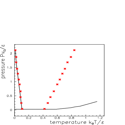
a)

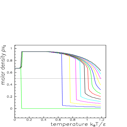
b)

Figure 2: MF phase diagram for the model in Eqs.(1,2) with $J/\epsilon=0.5$, $X/\epsilon=0.01$, $v_{HB}/v_{0}=0.25$, $\gamma=4$, $q=10$. a) The $P,T$ projection: Lines represent phase transitions with negatively sloped solid-liquid transition and liquid-gas transition ending in a critical point; Stars represent the limits of the TMD region. b) The $\rho,T$ projection for isobars ranging from $Pv_{0}/\epsilon=-.0007$ (bottom) to $Pv_{0}/\epsilon=0.36$ (up) with increment of $\Delta Pv_{0}/\epsilon=0.03$. Note that for $Pv_{0}/\epsilon=-.0007$ there is a solid-gas transition, that is indistinguishable in a).

It is to be noted here that in our approach we are ignoring the fluctuations and supposing that the Potts (orientational) symmetry breaking always occurs, therefore we cannot have a new transition line ending in a new critical point. The inclusion of fluctuations could be the essential feature to recover the second critical point in the metastable supercooled liquid phase. Furthermore at negative pressure and $T=0$ a spurious state appears, due to the strong assumption (the Potts symmetry breaking) that we made and to the fact that upon stretching the system can minimize the Gibbs free energy forming HBs in the gas phase.

Conclusions and Open Issues

By taking a simple model of water that leads to the singularity-free scenario Sastry96 ; Rebelo98 as interpretation of the anomalous water behavior and adding a term that correlates the intra-molecular orientational degrees of freedom, we recover the solid phase, the liquid-solid and the gas-solid transition lines. Furthermore the TMD “region” is above the melting line. All those are characteristic features of water not included in the seminal Sastry et al. model Sastry96 ; Rebelo98 . This can be considered a more realistic extension of the previously mapped singularity-free phase diagram, which has no such transitions. However, these are stable transitions which by themselves cannot verify or negate the existence of singularities in the metastable region, but they make the phase diagram more water-like.

So far our investigation is done only adding correlations between the orientational degrees of freedom in the limit of no fluctuations. In order to understand the critical phenomena of water in the supercooled region, thermal fluctuations cannot be ignored. An inherent shortcoming of MF calculations is that such fluctuations are blotted out by strong approximations. One way of including such fluctuations into the analysis is to consider them into the MF calculations in a perturbative manner, for instance by taking into account the local fluctuations of density Borick95 . Another way is to conduct numerical simulations Roberts96a . We will now pursue these two new paths to see what effect fluctuations have on the phase behavior of this system, particularly in the metastable region.

References

- (1) Speedy, R.J. and Angell, C.A. J. Chem. Phys. 65, 851 (1976).
- (2) Hare, D.E. and Sorensen, C.M., J. Chem. Phys. 87, 4840 (1987).
- (3) Angell, C.A., Oguni, M., and Sichina, W.J., J. Phys. Chem 86, 998 (1982).
- (4) Angell, C.A. in Water: A Comprehensive Treatise Franks F. ed., New York: Plenum, 1982, vol. 7, pp.1.
- (5) Bellissent-Funel, M.-C. ed., Hydration Processes in Biology. Theoretical and Experimental Approaches, Amsterdam: IOS Press, NATO ASI Series A, vol.305, 1998.
- (6) Bellissent-Funel, M.-C. and Bosio, L., J. Chem. Phys. 102, 3727 (1995).
- (7) Mishima, O. and Stanley, H.E., Nature 392, 164 (1998); ibidem 396, 329 (1998).
- (8) Smith R.S., Kay B.D., Nature 398, 788 (1999).
- (9) Shiratani, E. and Sasai, M., J. Chem. Phys. 108, 3264 (1998).
- (10) Debenedetti P.G., Metastable Liquids: Concepts and Principles, Princeton: Princeton Univerisity Press, 1998.
- (11) Ponyatovsky, E.G. and Pozdnyakova, T.A., J. Non-cryst. Solids 188, 153 (1995).
- (12) Roberts, C.J., Panagiotopulos A.Z. and Debenedetti, P.G., Phys. Rev. Lett. 77, 4386 (1996).
- (13) Roberts, C.J. and Debenedetti, P.G., J. Chem. Phys. 105, 658 (1996).
- (14) Sadr-Lahijany, M.R., Scala, A. Buldyrev, S.V. and Stanley, H.E., Phys. Rev. Lett. 81, 4895 (1998); Physical Review E 60, 6714 (1999).
- (15) Speedy, R.J., J. Phys. Chem. 86, 3002 (1982).
- (16) Poole, P.H., Sciortino, F., Essman, U., and Stanley, H.E., Nature 360, 324 (1992); see also Tanaka, H., J. Chem. Phys. 105, 5099 (1996), Harrington, S.T., Zhang, R., Poole, P.H., Sciortino, F., and Stanley, H.E.,J. Chem. Phys. 78, 2409 (1997), and Sciortino, F., Poole, P.H., Essmann, U. and Stanley, H.E.,Phys. Rev. E 55, 727 (1997).
- (17) Stanley, H.E. and Teixeira, J., J. Chem. Phys. 73, 3404 (1980).
- (18) Sastry, S., Debenedetti, P.G., Sciortino, F., and Stanley, H.E., Phys. Rev. E 53, 6144 (1996); La Nave E., Sastry S., Sciortino F., and Tartaglia P., Phys. Rev. E 59, 6348 (1999).
- (19) Rebelo L.P.N., Debenedetti P.G., Sastry S., J. Chem. Phys. 109, 626 (1998).
- (20) Poole, P.H., Sciortino, F., Grande, T., Stanley, H.E. and Angell, C.A., Phys. Rev. Lett. 73, 1632 (1994).
- (21) Borick, S.S., Debenedetti, P.G. and Sastry, S., J. Phys. Chem. 99, 3781 (1995).
- (22) Grimsditch, M., Phys. Rev. Lett. 52, 2379 (1984).
- (23) Smith, K.H., Shero, E., Chizmeshya, A., and Wolf, G.H., J. Chem. Phys. 102, 6851(1995).
- (24) Wu, F., Rev. Mod. Phys. 54, 235 (1982).