Critical behavior at $\boldsymbol{m}$-axial Lifshitz points: field-theory analysis and $\boldsymbol{\epsilon}$-expansion results

Abstract

The critical behavior of $d$-dimensional systems with an $n$-component order parameter is reconsidered at $(m,d,n)$-Lifshitz points, where a wave-vector instability occurs in an $m$-dimensional subspace of ${\mathbb{R}}^{d}$. Our aim is to sort out which ones of the previously published partly contradictory $\epsilon$-expansion results to second order in $\epsilon=4+\frac{m}{2}-d$ are correct. To this end, a field-theory calculation is performed directly in the position space of $d=4+\frac{m}{2}-\epsilon$ dimensions, using dimensional regularization and minimal subtraction of ultraviolet poles. The residua of the dimensionally regularized integrals that are required to determine the series expansions of the correlation exponents $\eta_{l2}$ and $\eta_{l4}$ and of the wave-vector exponent $\beta_{q}$ to order $\epsilon^{2}$ are reduced to single integrals, which for general $m=1,\ldots,d-1$ can be computed numerically, and for special values of $m$, analytically. Our results are at variance with the original predictions for general $m$. For $m=2$ and $m=6$, we confirm the results of Sak and Grest [Phys. Rev. B 17, 3602 (1978)] and Mergulhão and Carneiro’s recent field-theory analysis [Phys. Rev. B 59,13954 (1999)].

I Introduction

A Lifshitz point [3, 4, 5, 6] is a critical point at which a disordered phase, a spatially homogeneous ordered phase, and a spatially modulated phase meet. In the case of a $d$-dimensional system with an $n$-component order parameter, it is called an $(m,d,n)$-Lifshitz point (or $m$-axial Lifshitz point) if a wave-vector instability occurs in an $m$-dimensional subspace. Such multi-phase points are known to occur in a variety of distinct physical systems, including magnetic ones [7, 8], ferroelectric crystals [9], charge-transfer salts,[10, 11] liquid crystals,[12] systems undergoing structural phase transitions[13] or having domain-wall instabilities,[14] and the ANNNI model.[15, 16] A survey covering the work related to them till 1992 has been given by Selke,[6] which complements and updates an earlier review by Hornreich.[5] Recently there has also been renewed interest in the effects of surfaces on the critical behavior at Lifshitz points.[17, 18, 19]

From a general vantage point, critical behavior at Lifshitz points is an interesting subject in that it presents clear and simple examples of anisotropic scale invariance. Epitomized also by dynamic critical phenomena near thermal equilibrium,[20] and known to occur as well in other static equilibrium systems (e.g., uniaxial dipolar ferromagnets), this kind of invariance has gained increasing attention in recent years since it was found to be realized in many non-equilibrium systems such as driven diffusive systems [21] and in growth processes.[22]

Systems at Lifshitz points are good candidates for studying general aspects of anisotropic scale invariance.[23, 24] For one thing, the continuum theories representing the universality classes of systems with short-range interactions at $(m,d,n)$-Lifshitz points are conceptually simple; second, they involve the degeneracy $m$ as a parameter, which can easily be varied between $1$ and $d$. A thorough understanding of critical behavior at such Lifshitz points is clearly very desirable.

The problem has been studied decades ago by means of an $\epsilon$ expansion about the upper critical dimension[3, 25, 26, 27]

$$d^{*}(m)=4+\frac{m}{2}\;,\quad m\leq 8\,.$$ (1)

Other investigations employed the dimensionality expansion about the lower critical dimension[28] $d_{*}(m)=2+\frac{m}{2}$ for $n\geq 3$, or the $1/n$ expansion. [4, 29, 30] Unfortunately, the $\epsilon$-expansion results to order $\epsilon^{2}$ one group of authors[3, 25, 26] obtained for the correlation exponents $\eta_{l2}$ and $\eta_{l4}$ and the wave-vector exponent $\beta_{q}$ are in conflict with those of Sak and Grest[27] for the cases $m=2$ and $m=6$.

In order to resolve this long-standing controversy, Mergulhão and Carneiro[31, 32] recently presented a reanalysis of the problem based on renormalized field theory and dimensional regularization. Exploiting the form of the resulting renormalization-group equations, they were able to derive various (previously given) general scaling laws one expects to hold according to the phenomenological theory of scaling. However, their calculation of critical exponents was limited in a twofold fashion: They treated merely the special cases $m=2$ and $m=6$, in which considerable simplifications occur. Their results for $\eta_{l2}$ and $\eta_{l4}$ to order $\epsilon^{2}$, agree with Sak and Grest’s[27] but disagree with Mukamel’s.[25] Second, the exponent $\beta_{q}$ (an independent exponent that does not follow from these correlation exponents via a scaling law) was not considered at all by them. Thus it is an open question whether Sak and Grest’s or Mukamel’s ${\mathcal{O}}(\epsilon^{2})$ results for $\beta_{q}$ with $m=2$ and $m=6$ are correct. Furthermore, for other values of $m$, the published ${\mathcal{O}}(\epsilon^{2})$ results[25, 26] for the exponents $\eta_{l2}$, $\eta_{l4}$, and $\beta_{q}$ remain unchecked.

It is the purpose of this work to fill these gaps and to determine the $\epsilon$ expansion of the critical exponents $\eta_{l2}$, $\eta_{l4}$, and $\beta_{q}$ for general values of $m$ to order $\epsilon^{2}$.

Technically, we shall employ dimensional regularization in conjunction with minimal subtraction of poles in $\epsilon$. This way of fixing the counterterms appears to us somewhat more convenient than the use of normalization conditions (as was done in Refs. [31] and [32]). In order to overcome the rather demanding technical challenges, we have found it useful to work directly in position space. Thus the Laurent expansion of the distributions to which the Feynman graphs of the primitively divergent vertex functions correspond in position space must be determined to the required order in $\epsilon$.

The source of the technical difficulties is that these Feynman graphs, at criticality, involve a free propagator $G(\boldsymbol{x})$ which is a generalized homogeneous rather than a homogeneous function, because of the anisotropic scale invariance of the free theory. While such a situation is encountered also in other cases of anisotropic scale invariance, the scaling function associated with $G(\boldsymbol{x})$ turns out to be a particularly complicated function in the present case of a general $(m,d,n)$-Lifshitz point. (For general values of $m$, it is a sum of two generalized hypergeometric functions.)

In the next section, we recall the familiar continuum model describing the critical behavior at a $(m,d,n)$-Lifshitz point and discuss its renormalization. In Sec. III details of our calculation are presented, and our results for the renormalization factors are derived. Then renormalization-group equations are given in Sec. IV, which are utilized to deduce the general scaling form of the correlation functions, to identify the critical exponents, and to derive their scaling laws as well as the anticipated multi-scale-factor universality. This is followed by a presentation of our $\epsilon$-expansion results for the critical exponents $\eta_{l2}$, $\eta_{4l}$, and $\beta_{q}$. Sec. V contains a brief summary and concluding remarks. Finally, there are two appendices to which some computational details have been relegated.

II The Model and its Renormalization

We consider the standard continuum model representing the universality class of a $(m,d,n)$-Lifshitz point with the Hamiltonian

$${\mathcal{H}}[\boldsymbol{\phi}] = \frac{1}{2}\int d^{d}x\left\{\rho_{0}\left({\nabla\!_{\parallel}}\,\boldsymbol{\phi}\right)^{2}+{\sigma_{0}}\left({\Delta_{\parallel}}\boldsymbol{\phi}\right)^{2}\right.$$ (3)

$$\left.\mbox{}\qquad+\left({\nabla\!_{\perp}}\,\boldsymbol{\phi}\right)^{2}+{\tau_{0}}\,\boldsymbol{\phi}^{2}+\frac{u_{0}}{12}\,|\boldsymbol{\phi}|^{4}\right\}\;.$$

Here $\boldsymbol{\phi}(\boldsymbol{x})=(\phi_{1},\ldots,\phi_{n})$ is an $n$-component order-parameter field. The coordinate $\boldsymbol{x}\in{\mathbb{R}}^{d}$ has an $m$-dimensional parallel component, $\boldsymbol{x}_{\parallel}$, and a ($d-m$)-dimensional perpendicular one, $\boldsymbol{x}_{\perp}$. Likewise, $\nabla\!_{\parallel}$ and $\nabla\!_{\perp}$ denote the associated parallel and perpendicular components of the gradient operator ${\nabla}$, while $\Delta_{\parallel}$ means the Laplacian ${\nabla\!_{\parallel}}^{2}$. At the level of Landau theory, the Lifshitz point is located at $\rho_{0}=\tau_{0}=0$.

The Hamiltonian is invariant under the transformation

$$\boldsymbol{x}_{\parallel}\to a\,\boldsymbol{x}_{\parallel}\;,\;\;\boldsymbol{x}_{\perp}\to\boldsymbol{x}_{\perp}\;,\;\;\boldsymbol{\phi}\to a^{-m/2}\,\boldsymbol{\phi}\;,$$ (4)

$$\sigma_{0}\to a^{4}\,\sigma_{0}\;,\;\;\rho_{0}\to a^{2}\,\rho_{0}\;,\;\;\tau_{0}\to\tau_{0}\;,$$ (5)

$$u_{0}\to a^{m}\,u_{0}\;.$$ (6)

Thus, appropriate invariant interaction constants are $u_{0}\,{\sigma_{0}}^{-m/4}$, $\rho_{0}\,{\sigma_{0}}^{-1/2}$, and $\tau_{0}$, and the dependence on the parallel coordinates is through the invariant combination ${\sigma_{0}}^{-1/4}\,\boldsymbol{x}_{\parallel}$.

Dimensional analysis yields the dimensions $[.]$:

$$[x_{\parallel}] = [\sigma_{0}]^{{1/4}}\,\mu^{-{1/2}}\,,\quad[x_{\perp}]=\mu^{-1}\,,$$ (7)

$$[\tau_{0}] = \mu^{2}\,,\quad[\rho_{0}]=[\sigma_{0}]^{1/2}\,\mu\;,$$ (8)

$$[u_{0}] = [\sigma_{0}]^{m/4}\,\mu^{\epsilon}\;\mbox{ with }\;\epsilon=d^{*}(m)-d\;,$$ (9)

$$[\phi_{i}(\boldsymbol{x})] = [\sigma_{0}]^{-{m/8}}\,\mu^{\left(d-2-\frac{m}{2}\right)/2}\;,$$ (10)

where $\mu$ is an arbitrary momentum scale.

Let

$$G_{i_{1},\ldots,i_{N}}^{(N)}(\boldsymbol{x}_{1},\ldots,\boldsymbol{x}_{N})=\langle\phi_{i_{1}}(\boldsymbol{x}_{1})\ldots\phi_{i_{N}}(\boldsymbol{x}_{N})\rangle^{\mathrm{c}um}$$ (11)

denote the connected $N$-point correlation functions (cumulants) and $\Gamma_{i_{1},\ldots,i_{N}}^{(N)}(x_{1},\ldots,x_{N})$ the corresponding vertex functions. Using power counting one concludes that the ultraviolet (uv) singularities of these functions can be absorbed through the reparameterizations

$$\phi = {Z_{\phi}}^{{1}/{2}}\,\phi_{\mathrm{r}en}\;,$$ (13)

$$\tau_{0}-\tau_{0c} = \mu^{2}\,Z_{\tau}\,\tau\;,$$ (14)

$$\sigma_{0} = Z_{\sigma}\,\sigma\;,$$ (15)

$$u_{0}\,{\sigma_{0}}^{-m/4}\,A_{d,m} = \mu^{\epsilon}\,Z_{u}\,u\;,$$ (16)

$$\left(\rho_{0}-\rho_{0c}\right)\,{\sigma_{0}}^{-1/2} = \mu\,Z_{\rho}\,\rho\;,$$ (17)

where

$$A_{d,m}={S_{d-m}\,S_{m}}\,={4\,\pi^{d/2}\over\Gamma\big{(}{d-m\over 2}\big{)}\,\Gamma(m/2)}$$ (18)

is a convenient normalization factor we absorb in the renormalized coupling constant. Here

$$S_{D}=\frac{2\,\pi^{D/2}}{\Gamma(D/2)}$$ (19)

is the surface area of a $D$-dimensional unit sphere.

The quantities $\tau_{0c}$ and $\rho_{0c}$ correspond to shifts of the Lifshitz point. In our perturbative approach based on dimensional regularization they vanish. If we wanted to regularize the uv singularities via a cutoff $\Lambda$ (restricting the integrations over parallel and perpendicular momenta by $|{\boldsymbol{q}\/_{\parallel}}|\leq\Lambda$ and $|{\boldsymbol{q}\/_{\perp}}|\leq\Lambda$), they would be needed to absorb uv singularities quadratic and linear in $\Lambda$, respectively.

In the renormalization scheme we use, the renormalization factors $Z_{\phi}$, $Z_{\sigma}$, $Z_{\tau}$, $Z_{\rho}$, and $Z_{u}$, for given values of the parameters $\epsilon$, $n$, and $m$, depend just on the dimensionless renormalized coupling constant $u$; that is, they are independent of $\sigma$, $\tau$, and $\rho$. This follows from the fact that the primitive divergences of the momentum-space vertex functions $\tilde{\Gamma}^{(2)}(\boldsymbol{q})$ and $\tilde{\Gamma}^{(4)}(\boldsymbol{q}_{1},\ldots,\boldsymbol{q}_{1})$, at any order of $u_{0}\,{\sigma_{0}}^{-m/4}$, are poles in $\epsilon$ whose residua depend linearly on ${q_{\perp}}^{2}$, $\rho_{0}\,{q_{\parallel}}^{2}$, $\sigma_{0}\,{q_{\parallel}}^{4}$, and $\tau_{0}$ in the case of the former and are independent of these momenta and mass parameters in the case of the latter. Subtracting these poles minimally as usual implies that these renormalization factors differ from $1$ through Laurent series in $\epsilon$:

$$Z_{\iota} = 1+\sum_{p=1}^{\infty}{a_{\iota,p}^{(r)}(u;m,n)\,\epsilon^{-p}}$$ (20)

$$= 1+\sum_{r=1}^{\infty}\sum_{p=1}^{r}\,a_{\iota,p}^{(r)}(m,n)\,\frac{u^{r}}{\epsilon^{p}}\;,\;\;\iota=\phi,\,u,\,\tau,\,\sigma,\,\rho\,.$$ (21)

III Outline of Computation and Perturbative Results

We shall compute the leading nontrivial contributions to these renormalization factors. In the cases of $Z_{\phi}$, $Z_{\sigma}$, and $Z_{\rho}$, whose ${\mathcal{O}}(u)$ contributions vanish, these are of order $u^{2}$; for $Z_{u}$ and $Z_{\tau}$ they are of first order in $u$.

To this end we expand about the Lifshitz point, using the free propagator

$$G(\boldsymbol{x})=\int\limits_{\boldsymbol{q}}\,\frac{{\mathrm{e}}^{i(\boldsymbol{q}_{\parallel}\cdot\boldsymbol{x}_{\parallel}+\boldsymbol{q}_{\perp}\cdot\boldsymbol{x}_{\perp})}}{\sigma_{0}\,q_{\parallel}^{4}+q_{\perp}^{2}}\;.$$ (23)

Here the (dimensionally regularized) momentum-space integral is defined through

$$\int\limits_{\boldsymbol{q}}\ldots=\int\limits_{\boldsymbol{q}_{\parallel}}\int\limits_{\boldsymbol{q}_{\perp}}\ldots=\int\limits_{{\mathbb{R}}^{m}}\frac{d^{m}q}{(2\,\pi)^{m}}\!\int\limits_{{\mathbb{R}}^{d-m}}\frac{d^{d-m}q}{(2\,\pi)^{d-m}}\ldots\;.$$ (24)

Let $r_{\parallel}\equiv|\boldsymbol{x}_{\parallel}|$ and $r_{\perp}\equiv|\boldsymbol{x}_{\perp}|$. Then the free propagator can be written in the scaling form

$$G(\boldsymbol{x}) = {r_{\perp}}^{-2+\epsilon}\,\Phi\big{(}{\sigma_{0}}^{-1/4}\,{r_{\parallel}\,{r_{\perp}}^{-1/2}}\big{)}$$ (25)

with

$$\Phi(\upsilon)\equiv\Phi(\upsilon;m,d)=\int\limits_{\boldsymbol{q}}\,\frac{{\mathrm{e}}^{i(\boldsymbol{q}_{\parallel}\cdot\boldsymbol{\upsilon}+\boldsymbol{q}_{\perp}\cdot\boldsymbol{e}_{\perp})}}{q_{\parallel}^{4}+q_{\perp}^{2}}\;,$$ (26)

where $\boldsymbol{\upsilon}\in{\mathbb{R}}^{m}$ is a vector of length $\upsilon$ and arbitrary orientation, while $\boldsymbol{e}_{\perp}$ means the unit vector $\boldsymbol{x}_{\perp}/r_{\perp}$. Note that the scaling function $\Phi$ depends parametrically on $m$ and $d$. For the sake of brevity, we will usually suppress these variables, writing $\Phi(\upsilon;m,d)$ only when special values of $m$ and $d$ are chosen or when we wish to stress the dependence on these parameters.

The integration over $\boldsymbol{q}_{\perp}$ in (26) yields

$$\Phi(\upsilon)=(2\,\pi)^{-{d-m\over 2}}\,\int\limits_{\boldsymbol{q}_{\parallel}}\,{q_{\parallel}}^{d-m-2}\,{\mathrm{K}}_{\frac{d-m}{2}-1}({q_{\parallel}}^{2})\,{\mathrm{e}}^{i\,\boldsymbol{\upsilon}\cdot\boldsymbol{q}_{\parallel}}\;.$$ (27)

Upon introducing spherical coordinates $q=|\boldsymbol{q}_{\parallel}|$ and $\Omega^{(m)}=(\theta_{1},\ldots,\theta_{m-1})$ for $\boldsymbol{q}_{\parallel}$, with $d\Omega^{(m)}=\sin^{m-2}\theta_{m-1}\,d\theta_{m-1}\,d\Omega^{(m-1)}$, one can perform the angular integrations. This gives

$$\Phi(\upsilon)={\upsilon^{-\frac{m-2}{2}}\over(2\,\pi)^{{d/2}}}\,\int\limits_{0}^{\infty}\!dq\,q^{2-\epsilon}\,{\mathrm{J}}_{m-2\over 2}(q\upsilon)\,{\mathrm{K}}_{\frac{d-m}{2}-1}({q}^{2})\;.$$ (28)

The integral remaining in (28) can be expressed as a combination of generalized hypergeometric functions ${{{}_{1\!}{\mathrm{F}}_{2}}}$ (see Appendix A). For special values of $m$ and $d$, the result reduces to simple expressions, which we have gathered in Appendix A.

The leading loop corrections to the vertex functions $\Gamma^{(4)}$ and $\Gamma^{(2)}$ at the Lifshitz point are given in position space by the graphs pt 2.5 0.2 (-4 0) (0 3) (5 0) rx:5 ry:2 (-4.5 -1.2)$\boldsymbol{x}$ (11.5 -1.9)$\boldsymbol{y}$ (0 0) f:1 r:0.7 r:0.7 (10 0) f:1 r:0.7 r:0.7 (16.5 0) and pt 2.5 0.2 (-4 0) (0 3) (5 0) rx:5 ry:2 (10 0) (-10 0) (-4.5 -1.2)$\boldsymbol{x}$ (11.5 -1.9)$\boldsymbol{y}$ (0 0) f:1 r:0.7 r:0.7 (10 0) f:1 r:0.7 r:0.7 (16.5 0) , which are proportional to $G^{2}(\boldsymbol{x}-\boldsymbol{y})$ and $G^{3}(\boldsymbol{x}-\boldsymbol{y})$, respectively. Hence we must determine the Laurent expansion of these distributions. To this end we set $\sigma_{0}=1$ and consider the action $(G^{s},\varphi)$ of $G^{s}(\boldsymbol{x})$ for $s=2,3$ on a test function $\varphi(\boldsymbol{x})$. We substitute (25) for $G$ and use spherical coordinates $(r_{\parallel},\Omega_{\parallel})$ and $(r_{\perp},\Omega_{\perp})$ for the parallel and perpendicular components of $\boldsymbol{x}$, writing $\varphi(\boldsymbol{x})=\varphi(r_{\parallel},\Omega_{\parallel};r_{\perp},\Omega_{\perp})$. We thus obtain

$$\left(G^{s},\varphi\right) = \left({r_{\perp}}^{-s(2-\epsilon)}\,\Phi^{s}\big{(}{r_{\parallel}\,{r_{\perp}}^{-1/2}}\big{)},\varphi\right)$$ (29)

$$= \int\!d^{d}x\,{r_{\perp}}^{-s(2-\epsilon)}\,\Phi^{s}\big{(}{r_{\parallel}\,{r_{\perp}}^{-1/2}}\big{)}\,\varphi(\boldsymbol{x})$$ (30)

$$= \int\!d^{d-m}x_{\perp}\;{r_{\perp}}^{-s(2-\epsilon)+\frac{m}{2}}\,\psi_{s}(\boldsymbol{x}_{\perp})\;,$$ (31)

where the functions $\psi_{s}(\boldsymbol{x}_{\perp})\equiv\psi_{s}(r_{\perp},\Omega_{\perp})$ are defined through

$$\psi_{s}(\boldsymbol{x}_{\perp})=\int\!d^{m}{x_{\parallel}}\,\Phi^{s}\big{(}r_{\parallel}\big{)}\,\varphi\big{(}r_{\parallel}\,\sqrt{r_{\perp}},\Omega_{\parallel};r_{\perp},\Omega_{\perp}\big{)}\,.$$ (32)

The final result in (29) is the linear functional $\left({r_{\perp}}^{-s(2-\epsilon)+\frac{m}{2}},\psi_{s}\right)$. Generalized functions such as ${r_{\perp}}^{(\ldots)}$ and their Laurent expansions are discussed in Ref. [33]. Let $\psi(\boldsymbol{x}_{\perp})\equiv\psi(r_{\perp},\Omega_{\perp})$ be a smooth ($C^{\infty}$) test function on ${\mathbb{R}}^{d-m}$ and

$$\overline{\psi}^{\Omega_{\perp}}(r_{\perp})\equiv\frac{1}{S_{d-m}}\,\int\!d\Omega_{\perp}\,\psi(r_{\perp},\Omega_{\perp})$$ (33)

its spherical average. Then we have

$$\left({r_{\perp}}^{-s(2-\epsilon)+\frac{m}{2}},\psi\right) \equiv \int\!d^{d-m}{x_{\perp}}\,{r_{\perp}}^{-s(2-\epsilon)+\frac{m}{2}}\,\psi(\boldsymbol{x}_{\perp})$$ (34)

$$= S_{d-m}\,\int\limits_{0}^{\infty}\!dr\,{r}^{3-2\,s+\epsilon(s-1)}\,\overline{\psi}^{\Omega_{\perp}}(r)$$ (35)

$$= S_{d-m}\,\left({r_{+}}^{3-2\,s+\epsilon(s-1)},\overline{\psi}^{\Omega_{\perp}}\right)\,.$$ (36)

Here ${r_{+}}^{\lambda}$ is a standard generalized function in the notation of Ref. [33]. Its Laurent expansion about the pole at $\lambda=-p=-1,-2,\ldots$ reads

$${r_{+}}^{\lambda}=\frac{(-1)^{p-1}}{(p-1)!}\,\frac{\delta^{(p-1)}(r)}{\lambda+p}+{r_{+}}^{-p}+{\mathcal{O}}(\lambda+p)\;,$$ (38)

where the generalized function ${r_{+}}^{-p}$ is defined by

$$\left({r_{+}}^{-p},\varphi(r)\right) = \int\limits_{0}^{\infty}\!dr\,{r_{+}}^{-p}\biggl{[}\varphi(r)-\sum_{j=0}^{p-2}\frac{r^{j}}{j!}\,\varphi^{(j)}(0)$$ (40)

$$\mbox{}-\frac{r^{p-1}}{(p-1)!}\,\varphi^{(p-1)}(0)\,\theta(1-r)\biggr{]}.$$

Using these results, the leading terms of the Laurent expansions of $(G^{s},\varphi)$ can be determined in a straightforward manner. However, it should be noted that the functions $\psi_{s}(\boldsymbol{x}_{\perp})$ introduced in (32) are not a priori guaranteed to have the usually required strong properties of test functions (continuous partial derivatives of all orders and sufficiently fast decay as $|\boldsymbol{x}_{\perp}|\to\infty$). In particular, one may wonder whether the dependence on the variable $r_{\parallel}\,\sqrt{r_{\perp}}$ of $\varphi$ in (32) does not imply that derivatives such as $\nabla_{\perp}\psi_{s}$ become singular at the origin. Closer inspection reveals that this is not the case since the problematic term $\sim{r_{\perp}}^{-1}$ involves the vanishing angular integral $\int\!d\Omega_{\parallel}\,\boldsymbol{x}_{\parallel}\,\varphi(\ldots)$.

One obtains

$${\left(G^{2},\varphi\right)\over S_{d-m}}=\bigg{[}\frac{\psi_{2}(\boldsymbol{0})}{\epsilon}+\left({r_{+}}^{-1},\overline{\psi_{2}}^{\Omega_{\perp}}(r)\right)+{\mathcal{O}}(\epsilon)\bigg{]}$$ (41)

and

$${\left(G^{3},\varphi\right)\over S_{d-m}}=\bigg{[}\frac{{\overline{\psi_{3}}^{\Omega_{\perp}}}^{\prime\prime}(0)}{4\,\epsilon}+\left({r_{+}}^{-3},\overline{\psi_{3}}^{\Omega_{\perp}}(r)\right)+{\mathcal{O}}(\epsilon)\bigg{]}.$$ (42)

From its definition in (32) we see that the residuum $\psi_{2}(\boldsymbol{0})$ on the right-hand side of (41) reduces to a simple expression $\propto\varphi(\boldsymbol{0})$. We thus arrive at the expansion

$${G^{2}(\boldsymbol{x})\over A_{d,m}}=\frac{J_{0,2}(m,d^{*})}{\epsilon}\,\delta(\boldsymbol{x})\,+{\mathcal{O}}(\epsilon^{0})\;,$$ (43)

where $J_{0,2}$ is a particular one of the integrals

$$J_{p,s}(m,d)\equiv\int\limits_{0}^{\infty}\!\upsilon^{m-1+p}\,\Phi^{s}(\upsilon;m,d)\,d\upsilon\;.$$ (44)

In order to convert the Laurent expansion (42) into one for $G^{3}(\boldsymbol{x})$, we must compute ${\overline{\psi_{3}}^{\Omega_{\perp}}}^{\prime\prime}(0)$. This in turn requires the calculation of the following angular average:

$$\left.{\partial^{2}\over\partial r^{2}}\,\overline{\varphi\big{(}r_{\parallel}\sqrt{r},\Omega_{\parallel};r,\Omega_{\perp}\big{)}}^{\Omega_{\parallel},\Omega_{\perp}}\right|_{r=0}$$ (45)

$$= \frac{2}{4!}\,\overline{\left(\boldsymbol{x}_{\parallel}\cdot\nabla_{\parallel}\right)^{4}\,\varphi(\boldsymbol{0})}^{\Omega_{\parallel},\Omega_{\perp}}+\overline{\left(\boldsymbol{e}_{\perp}\cdot\nabla_{\perp}\right)^{2}\,\varphi(\boldsymbol{0})}^{\Omega_{\parallel},\Omega_{\perp}}$$ (46)

$$= \frac{{r_{\parallel}}^{4}\,({\triangle_{\parallel}}^{2}\varphi)(\boldsymbol{0})}{4m(m+2)}+\frac{(\triangle_{\perp}\varphi)(\boldsymbol{0})}{d-m}\;.$$ (47)

Using this in conjunction with (42) gives

$${G^{3}(\boldsymbol{x})\over A_{d,m}} = {J_{4,3}(m,d^{*})\,{\triangle_{\parallel}}^{2}\delta(\boldsymbol{x})\over 16\,m(m+2)\,\epsilon}$$ (49)

$$\mbox{}+{J_{0,3}(m,d^{*})\,{\triangle_{\perp}}\delta(\boldsymbol{x})\over 4\,(d^{*}-m)\,\epsilon}+{\mathcal{O}}(\epsilon^{0})\,.$$

In order to compute the ${\mathcal{O}}(u^{2})$ term of $Z_{\rho}$, we consider the two-point vertex function with an insertion of the operator $\frac{1}{2}\int d^{d}x({\nabla_{\|}}\phi)^{2}$ (to which $\rho_{0}$ couples). We represent such an insertion by the vertex pt 2.5 0.2 (5 2) f:0 r:0.7 (3.85 1)(0 2) (6.15 1)(0 2) (3 2) (4 0) (8 2) . At the Lifshitz point $\tau=\rho=0$, the leading nontrivial contribution to this vertex function is given by the two-loop graph pt 2.5 0.2 (-5 0) (0 3) (5 0) rx:5 ry:2 (5 2) f:0 r:0.7 (3.85 1)(0 2) (6.15 1)(0 2) (10 0) (-10 0) (10 0) f:1 r:0.7 r:0.7 (0 0) f:1 r:0.7 r:0.7 (-4.5 -1.2)$\boldsymbol{x}$ (11.5 -1.2)$\boldsymbol{0}$ (15.5 0) . The upper line involves the convolution

$$-(\nabla_{\|}G*{\nabla_{\|}}G)(\boldsymbol{x})={r_{\perp}}^{-1+\epsilon}\,\Xi\big{(}{\sigma_{0}}^{-1/4}\,{r_{\parallel}\,{r_{\perp}}^{-1/2}}\big{)}\,,$$ (50)

where

$$\Xi(\upsilon)\equiv\Xi(\upsilon;m,d)=\int\limits_{\boldsymbol{q}}\,\frac{{q_{\|}}^{2}\,{\mathrm{e}}^{i(\boldsymbol{q}_{\parallel}\cdot\boldsymbol{\upsilon}+\boldsymbol{q}_{\perp}\cdot\boldsymbol{e}_{\perp})}}{\left({q_{\parallel}}^{4}+{q_{\perp}}^{2}\right)^{2}}$$ (51)

is the analog of the scaling function $\Phi(\upsilon)$ (cf. (25)). Proceeding as in the case of the latter, one obtains

$$\Xi(\upsilon) = \frac{1}{2\,(2\pi)^{{d-m\over 2}}}\int\limits_{\boldsymbol{q}_{\|}}\!{q_{\parallel}}^{d-m-2}\,{\mathrm{K}}_{\frac{d-m-4}{2}}({q_{\parallel}}^{2})\,{\mathrm{e}}^{i\,\boldsymbol{\upsilon}\cdot\boldsymbol{q}_{\parallel}}$$ (52)

$$= {\upsilon^{-\frac{m-2}{2}}\over 2\,(2\,\pi)^{{d/2}}}\,\int\limits_{0}^{\infty}\!dq\,q^{2-\epsilon}\,{\mathrm{J}}_{m-2\over 2}(q\upsilon)\,{\mathrm{K}}_{\frac{d-m-4}{2}}({q}^{2})\;.$$ (53)

The remaining single integral can again be expressed in terms of generalized hypergeometric functions. The corresponding general expression, as well as the simpler ones to which this reduces for special values of $m$ and $d$, may be found in Appendix A).

The required graph pt 2.5 0.2 (-5 0) (0 3) (5 0) rx:5 ry:2 (5 2) f:0 r:0.7 (3.85 1)(0 2) (6.15 1)(0 2) (10 0) (-10 0) (10 0) f:1 r:0.7 r:0.7 (0 0) f:1 r:0.7 r:0.7 (-4.5 -1.2)$\boldsymbol{x}$ (11.5 -1.2)$\boldsymbol{0}$ (15.5 0) is proportional to the distribution

$$D(\boldsymbol{x})=-G^{2}(\boldsymbol{x})\,({\nabla_{\|}}G*{\nabla_{\|}}G)(\boldsymbol{x})\;.$$ (55)

whose pole term can be worked out in a straightforward fashion by the techniques employed above. One finds

$$\frac{-G^{2}(\boldsymbol{x})\,({\nabla_{\|}}G*{\nabla_{\|}}G)(\boldsymbol{x})}{A_{d,m}}={I_{1}(m,d^{*})\,{\triangle_{\parallel}}\delta(\boldsymbol{x})\over 4\,m\,\epsilon}+{\mathcal{O}}(\epsilon^{0})$$ (56)

with

$$I_{1}(m,d)\equiv\int\limits_{0}^{\infty}\!\upsilon^{m+1}\,\Phi^{2}(\upsilon;m,d)\,\Xi(\upsilon;m,d)\,d\upsilon\;.$$ (57)

A convenient way of computing the renormalization factor $Z_{\tau}$ is to consider the vertex function $\Gamma^{(2,1)}$ with a single insertion of the operator $\frac{1}{2}\,\phi(\boldsymbol{y})^{2}$, which we depict as pt 2.5 0.2 (5 2) f:0 r:0.7 (3.5 2) (3 0) (-1.5 0) (0.5 0.5) (0 2.5) (3.6 5)$\boldsymbol{y}$ (7.5 2) (3.6 7) . Its one-loop contribution pt 2.5 0.2 (-5 0) (0 2) rx:4 ry:2 (0 0) f:1 r:0.7 r:0.7 (0 4) f:0 r:0.7 (0.5 0.5) (0 2.5) (-3 4.4)$\boldsymbol{y}$ (-1.35 -2.9)$\boldsymbol{x}$ (5 0)(0 -3.5) is proportional to $G^{2}(\boldsymbol{x}-\boldsymbol{y})$. Hence its Laurent expansion follows from that of the latter quantity.

Let us introduce coefficients $b_{\iota}(m)$ for the leading nontrivial contributions to the renormalization factors $Z_{\iota}$, writing these in the form

$$Z_{u}=1+b_{u}(m)\,\frac{n{+}8}{9}\,\frac{u}{\epsilon}+{\mathcal{O}}(u^{2})\;,$$ (58)

$$Z_{\tau}=1+b_{\tau}(m)\,\frac{n{+}2}{3}\,\frac{u}{\epsilon}+{\mathcal{O}}(u^{2})\;,$$ (59)

and

$$Z_{\varsigma}=1+b_{\varsigma}(m)\,\frac{n{+}2}{3}\,\frac{u^{2}}{\epsilon}+{\mathcal{O}}(u^{3})\;,\quad\varsigma=\phi,\sigma,\rho\,.$$ (60)

From the pole terms of $G^{2}(\boldsymbol{x}-\boldsymbol{y})$ given in (43) one easily deduces that

$$b_{u}(m)=3\,b_{\tau}(m)=\frac{3}{2}\,J_{0,2}(m,d^{*})\;.$$ (61)

The pole terms proportional to ${\triangle_{\perp}}\delta(\boldsymbol{x})$, ${\triangle_{\parallel}}^{2}\,\delta(\boldsymbol{x})$, and ${\triangle_{\parallel}}\,\delta(\boldsymbol{x})$ of the two-loop graphs considered above are absorbed by counterterms involving the renormalization factors $Z_{\phi}$, $\check{Z}_{\sigma}\equiv Z_{\sigma}\,Z_{\phi}$, and $\check{Z}_{\rho}\equiv Z_{\rho}\,Z_{\phi}\,{Z_{\sigma}}^{1/2}$, respectively. Utilizing the Laurent expansions (49) and (55), one finds that their coefficients are given by

$$b_{\phi}(m)=-{1\over 24}\,{1\over d^{*}{-}m}\,{J_{0,3}(m,d^{*})\over A_{d^{*},m}}\;,$$ (62)

$$\check{b}_{\sigma}(m)={1\over 96}\,{1\over m(m{+}2)}\,\frac{J_{4,3}(m,d^{*})}{A_{d^{*},m}}\;,$$ (63)

and

$$\check{b}_{\rho}(m)={1\over 8m}\,\frac{I_{1}(m,d^{*})}{A_{d^{*},m}}\;.$$ (64)

The coefficients $b_{\sigma}$ and $b_{\rho}$ are related to these via

$$b_{\sigma}(m)=\check{b}_{\sigma}(m)-b_{\phi}(m)$$ (65)

and

$$b_{\rho}(m)=\check{b}_{\rho}(m)-{1\over 2}\,b_{\phi}(m)-{1\over 2}\,\check{b}_{\sigma}(m)\;.$$ (66)

IV Renormalization Group Equations and $\boldsymbol{\epsilon}$-Expansion Results

The reparameterizations (11) yield the following relations between bare and renormalized correlation and vertex functions

$$G^{(N)}(\boldsymbol{x}_{\parallel},\boldsymbol{x}_{\perp}) = {Z_{\phi}}^{N/2}\,G_{\mathrm{ren}}^{(N)}(\boldsymbol{x}_{\parallel},\boldsymbol{x}_{\perp})\;,$$ (68)

$$\Gamma^{(N)}(x_{\parallel},x_{\perp}) = {Z_{\phi}}^{-N/2}\,\Gamma_{\mathrm{ren}}^{(N)}(x_{\parallel},x_{\perp})\;,$$ (69)

where $\boldsymbol{x}_{\parallel}$ and $\boldsymbol{x}_{\perp}$ stand for the set of all parallel and perpendicular coordinates on which $G^{(N)}$ and $\Gamma^{(N)}$ depend. For conciseness, we have suppressed the tensorial indices $i_{1},\ldots,i_{N}$ of these functions and will generally do so below.

Upon exploiting the invariance of the bare functions under a change $\mu\to\bar{\mu}(\ell)=\mu\,\ell$ of the momentum scale in the usual fashion, one arrives at the renormalization-group equations

$$\left[{\mathcal{D}}_{\mu}+\frac{N}{2}\,\eta_{\phi}\right]G_{\mathrm{r}en}^{(N)} = 0\;,$$ (70)

$$\left[{\mathcal{D}}_{\mu}-\frac{N}{2}\,\eta_{\phi}\right]\Gamma_{\mathrm{r}en}^{(N)} = 0$$ (71)

with

$${\mathcal{D}}_{\mu} = \mu\,\partial_{\mu}+\beta_{u}\,\partial_{u}-\eta_{\sigma}\,\sigma\,\partial_{\sigma}$$ (73)

$$-(2+\eta_{\tau})\,\tau\,\partial_{\tau}-(1+\eta_{\rho})\,\rho\,\partial_{\rho}\;,$$

where the beta and eta functions are defined by

$$\beta_{u} \equiv \left.\mu\,\partial_{\mu}\right|_{0}u=-u\,\left[\epsilon+\eta_{u}(u)\right]$$ (74)

and

$$\eta_{\iota}\equiv\left.\mu\,\partial_{\mu}\right|_{0}\ln Z_{\iota}\;,\quad\iota=\phi,\,\sigma,\,\rho,\,\tau,\,u\;,$$ (75)

respectively. Here $\left.\partial_{\mu}\right|_{0}$ means a derivative at fixed bare variables $\mu_{0}$, $\rho_{0}$, $\sigma_{0}$, and $\tau_{0}$. Owing to our use of the minimal subtraction procedure, the functions $\eta_{\iota}$ can be expressed in terms of the residua $a_{\iota,1}(u;m,n)$ as

$$\eta_{\iota}(u)=-u\,\frac{da_{\iota,1}}{du}\;,\quad\iota=\phi,\,\sigma,\,\rho,\,\tau,\,u.$$ (76)

To solve the renormalization-group equations (IV) via characteristics, we introduce flowing variables through

$$\ell\,\frac{d}{d\ell}\,\bar{u}(\ell)=\beta_{u}[\bar{u}(\ell)]\;,\quad\bar{u}(1)=u\;,$$ (77)

$$\ell\,\frac{d}{d\ell}\,\bar{\sigma}(\ell)=-\eta_{\sigma}(\bar{u})\,\sigma\;,\quad\bar{\sigma}(1)=\sigma\;,$$ (78)

$$\ell\,\frac{d}{d\ell}\,\bar{\rho}(\ell)=-\left[1+\eta_{\rho}(\bar{u})\right]\rho\;,\quad\bar{\rho}(1)=\rho\;,$$ (79)

and

$$\ell\,\frac{d}{d\ell}\,\bar{\tau}(\ell)=-\left[2+\eta_{\tau}(\bar{u})\right]\tau\;,\quad\bar{\tau}(1)=\tau\;.$$ (80)

The flow equation (77) for the running coupling constant $\bar{u}(\ell)$ can be solved for $\ell$ to obtain

$$\ln\ell=\int\limits_{u}^{\bar{u}}\!{dx\over\beta_{u}(x)}\;.$$ (81)

For $\epsilon>0$, the beta function $\beta_{u}(u)$ is known to have a nontrivial zero $u^{*}$, corresponding to an infrared-stable fixed point. Expanding about this fixed point gives the familiar asymptotic form

$$\bar{u}(\ell)\mathop{=}\limits_{\ell\to 0}u^{*}+(u-u^{*})\,{\ell}^{\omega_{u}}+{\mathcal{O}}(\ell^{2\,\omega_{u}})$$ (82)

in the infrared limit $\ell\to 0$, where

$$\omega_{u}\equiv\frac{d\beta_{u}}{du}(u^{*})$$ (83)

is positive.

The solutions to the other flow equations, (78)–(80), can be conveniently written in terms of the anomalous dimensions $\eta_{\iota}^{*}\equiv\eta_{\iota}(u^{*})$ and the renormalization-group-trajectory integrals

$$E_{\iota}[\bar{u},u]=\exp\left\{\int\limits_{u}^{\bar{u}(\ell)}\!{dx}\,{\eta_{\iota}^{*}-\eta_{\iota}(x)\over\beta_{u}(x)}\right\}\;,\;\;\iota=\phi,\,\sigma,\,\rho,\,\tau\,,$$ (84)

which approach nonuniversal constants

$$E_{\iota}^{*}(u)\equiv E_{\iota}(u^{*},u)\;,\;\;\iota=\phi,\,\sigma,\,\rho,\,\tau\,,$$ (85)

in the infrared limit $\ell\to 0$.

One finds

$$\bar{\sigma}(\ell) = \ell^{-\eta_{\sigma}^{*}}\,E_{\sigma}[\bar{u}(\ell),u]\,\sigma$$ (86)

$$\mathop{\approx}\limits_{\ell\to 0} \ell^{-\eta_{\sigma}^{*}}\,E_{\sigma}^{*}(u)\,\sigma\;,$$ (87)

$$\bar{\rho}(\ell) = \ell^{-(1+\eta_{\rho}^{*})}\,E_{\rho}[\bar{u}(\ell),u]\,\rho$$ (88)

$$\mathop{\approx}\limits_{\ell\to 0} \ell^{-(1+\eta_{\rho}^{*})}\,E_{\rho}^{*}(u)\,\rho\;,$$ (89)

and

$$\bar{\tau}(\ell) = \ell^{-(2+\eta_{\tau}^{*})}\,E_{\tau}[\bar{u}(\ell),u]\,\tau$$ (90)

$$\mathop{\approx}\limits_{\ell\to 0} \ell^{-(2+\eta_{\tau}^{*})}\,E_{\tau}^{*}(u)\,\tau\;.$$ (91)

Solving the RG equation (68) in terms of characteristics yields

$$G^{(N)}_{\mathrm{r}en}(\boldsymbol{x}_{\parallel},\boldsymbol{x}_{\perp};\rho,\tau,u,\sigma,\mu)=\left[{\ell^{\eta_{\phi}^{*}}\over E_{\phi}(\bar{u},u)}\right]^{N/2}G^{(N)}_{\mathrm{r}en}(\boldsymbol{x}_{\parallel},\boldsymbol{x}_{\perp};\bar{\rho},\bar{\tau},\bar{u},\bar{\sigma},\mu\,\ell)$$ (92)

$$\quad=\left[{(\mu\,\ell)^{d-2-{m\over 2}}\,\ell^{\eta_{\phi}^{*}}\over\bar{\sigma}^{m/4}\,E_{\phi}(\bar{u},u)}\right]^{N/2}G^{(N)}_{\mathrm{r}en}\!\left[\left({\mu^{2}\,\ell^{2}/{\bar{\sigma}}}\right)^{1/4}\,\boldsymbol{x}_{\parallel},\mu\,\ell\,\boldsymbol{x}_{\perp};\bar{\rho},\bar{\tau},\bar{u},1,1\right]\;.$$ (93)

To obtain the second equality, we have used the relation

$$G^{(N)}_{\mathrm{r}en}(\boldsymbol{x}_{\parallel},\boldsymbol{x}_{\perp};\bar{\rho},\bar{\tau},\bar{u},\bar{\sigma},\bar{\mu}) = \left[\bar{\mu}^{d-2-\frac{m}{2}}\,\bar{\sigma}^{-m/4}\right]^{N/2}\,G^{(N)}_{\mathrm{r}en}(\bar{\sigma}^{-1/4}\,\bar{\mu}^{1/2}\,\boldsymbol{x}_{\parallel},\bar{\mu}\,\boldsymbol{x}_{\perp};\bar{\rho},\bar{\tau},\bar{u},1,1)\;,$$ (94)

implied by our dimensional considerations (7).

Let us assume that the function $G^{(N)}_{\mathrm{r}en}$ on the right-hand side of (92) has a nonvanishing limit $\bar{u}\to u^{*}$ for $\epsilon>0$. This assumption is in conformity with, and can be checked by, RG-improved perturbation theory. We choose $\ell=\ell_{\tau}$ such that

$$\bar{\tau}(\ell_{\tau})=\pm 1\quad\mbox{ for }\pm\tau>0$$ (95)

and consider the limit $\tau\to 0\pm$. To write the resulting asymptotic form of $G^{(N)}_{\mathrm{r}en}$ in a compact fashion, we introduce the correlation-length exponents

$$\nu_{l2}=\frac{1}{2+\eta_{\tau}^{*}}$$ (96)

and

$$\nu_{l4}=\frac{2+\eta_{\sigma}^{*}}{4(2+\eta_{\tau}^{*})}\;,$$ (97)

the crossover exponent

$$\varphi=\nu_{l2}\,(1+\eta_{\rho}^{*})\;,$$ (98)

as well as the correlation lengths

$$\xi_{\perp}\equiv\mu^{-1}\,\ell_{\tau}\approx\mu^{-1}\,\left[E_{\tau}^{*}(u)\,|\tau|\right]^{-\nu_{l2}}$$ (99)

and

$$\xi_{\parallel}\equiv\left[{\bar{\sigma}(\ell_{\tau})\over\mu^{2}\,{\ell_{\tau}}^{2}}\right]^{1/4}\approx\mu^{-1/2}\,\left[E_{\sigma}^{*}(u)\,\sigma\right]^{1/4}\,\left[E_{\tau}^{*}(u)\,|\tau|\right]^{-\nu_{l4}}\;.$$ (100)

In terms of these quantities the asymptotic critical behavior of $G^{(N)}_{\mathrm{r}en}$ becomes

$$G^{(N)}_{\mathrm{r}en}(\boldsymbol{x}_{\parallel},\boldsymbol{x}_{\perp};\rho,\tau,u,\sigma,\mu)\approx\left[{\mu^{-\eta_{\phi}^{*}}\over{E_{\phi}^{*}}}\,{\xi_{\perp}}^{-(d-m-2+\eta_{\phi}^{*})}\,{\xi_{\parallel}}^{-m}\right]^{N/2}{\mathcal{G}}_{\pm}^{(N)}\!\left[{\boldsymbol{x}_{\parallel}\over\xi_{\parallel}},{\boldsymbol{x}_{\perp}\over\xi_{\perp}};E_{\rho}^{*}\,\rho\,(\mu\,\xi_{\perp})^{\varphi/\nu_{l2}}\right]$$ (101)

with

$${\mathcal{G}}_{\pm}^{(N)}(\boldsymbol{x}_{\parallel},\boldsymbol{x}_{\perp};\rho)\equiv G^{(N)}_{\mathrm{r}en}(\boldsymbol{x}_{\parallel},\boldsymbol{x}_{\perp};\rho,\pm 1,u^{*},1,1)\;.$$ (102)

The result is the scaling form expected according to the phenomenological theory of scaling. As it shows, the scaling function ${\mathcal{G}}_{\pm}^{(N)}$ is universal, up to a redefinition of the nonuniversal metric factors associated with the relevant scaling fields, i.e., $E_{\sigma}^{*}$, $E_{\rho}^{*}$, $E_{\tau}^{*}$, and $E_{\phi}^{*}$. (Note that $E_{\phi}^{*}$, whose change would affect the overall amplitude of ${\mathcal{G}}_{\pm}^{(N)}$, as usual corresponds to a metric factor associated with the magnetic scaling field; see, e.g., Ref. [34].)

The correlation exponents $\eta_{l2}$ and $\eta_{l4}$ are given by

$$\eta_{l2}=\eta_{\phi}^{*}$$ (103)

and

$$\eta_{l4}=4\,\frac{\eta_{\sigma}^{*}+\eta_{\phi}^{*}}{2+\eta_{\sigma}^{*}}\;.$$ (104)

This can be seen either by taking the Fourier transform of the above result (101) with $N=2$ or else by solving directly the renormalization-group equation of $\tilde{\Gamma}^{(2)}_{\mathrm{r}en}({\boldsymbol{q}}_{\parallel},{\boldsymbol{q}}_{\perp})$. In order to identify the wave-vector exponent $\beta_{q}$, we utilize the scaling form

$$\tilde{\Gamma}^{(2)}_{\mathrm{r}en}({\boldsymbol{q}}_{\parallel},{\boldsymbol{q}}_{\perp};\tau,\rho,u)\approx|\tau|^{\gamma}\;\Upsilon_{\pm}(q_{\parallel}\xi_{\|},q_{\perp}\xi_{\perp};\rho\,|\tau|^{-\varphi})$$ (105)

of the inverse susceptibility $\tilde{\Gamma}^{(2)}$ and argue as in Ref. [25]: On the helical branch $T_{\text{hel}}(\rho)$ of the critical line, the inverse susceptibility vanishes at $\boldsymbol{q}_{c}=(\boldsymbol{q}^{c}_{\|},\boldsymbol{0})\neq\boldsymbol{0}$. Hence in the scaling regime, the line $T_{\text{hel}}(\rho)$ is determined by the zeroes of the scaling function $\Upsilon(p,0,\varrho)$. Denoting these as $p_{c}$ and $\varrho_{c}$, we obtain the relations

$$q^{c}_{\|}={p_{c}\,{\xi_{\|}}^{-1}}\sim p_{c}|\tau|^{\nu_{l4}}$$ (106)

and

$$\rho=\varrho_{c}|\tau|^{\varphi}\;,$$ (107)

which yield

$$q_{\|}^{c}\sim|\tau|^{\beta_{q}}$$ (108)

with

$$\beta_{q}=\frac{\nu_{l4}}{\varphi}=\frac{2+\eta_{\sigma}^{*}}{4(1+\eta_{\rho}^{*})}\;,$$ (109)

where the last equality follows upon substitution of (98) and (97) for $\varphi$ and $\nu_{l4}$, respectively.

To compute the exponent functions (75) and the beta function (74), we insert the residua of the renormalization factors (58)–(60) into (76) and express $b_{\tau}$ in terms of $b_{u}$ using (61). We thus obtain

$$\eta_{\varsigma}(u)=-2\,{n{+}2\over 3}\,b_{\varsigma}(m)\,u^{2}+{\mathcal{O}}(u^{3})\,,\quad\varsigma=\phi,\sigma,\rho\,,$$ (110)

$$\eta_{\tau}(u)=-{1\over 3}\,\frac{n{+}2}{3}\,b_{u}(m)\,u+{\mathcal{O}}(u^{2})\;,$$ (111)

and

$$\beta_{u}(u)=-u\left[\epsilon-\frac{n{+}8}{9}\;b_{u}(m)\,u+{\mathcal{O}}(u^{2})\right].$$ (112)

From the last equation we can read off the $\epsilon$ expansion of $u^{*}$, the nontrivial zero of $\beta_{u}$:

$$u^{*}={9\over n{+}8}\,{\epsilon\over b_{u}(m)}+{\mathcal{O}}\big{(}\epsilon^{2}\big{)}\,.$$ (113)

Evaluation of the above exponent functions at this fixed-point value gives us the $\epsilon$ expansions of the anomalous dimensions $\eta_{\iota}^{*}$. Substituting these into the expressions (96)–(98), (103), (104), and (109) for the critical exponents yields

$$\nu_{l2}={1\over 2}+{n{+}2\over 4(n{+}8)}\,\epsilon+{\mathcal{O}}(\epsilon^{2})\;,$$ (114)

$$\frac{\nu_{l4}}{\nu_{l2}} = \frac{1}{2}+{27(n{+}2)\over(n{+}8)^{2}}\;{b_{\phi}(m){-}\check{b}_{\sigma}(m)\over{2\,b_{u}(m)}^{2}}\;\epsilon^{2}+{\mathcal{O}}(\epsilon^{3})$$ (115)

$$= \frac{1}{2}+{\mathcal{O}}(\epsilon^{3})-{27(n{+}2)\over(n{+}8)^{2}}\,{\epsilon^{2}\over 4}\cases{0.02152&for $m=1$,\cr 0.02195&for $m=2$,\cr 0.02231&for $m=3$,\cr 0.02263&for $m=4$,\cr 0.02290&for $m=5$,\cr 0.02313&for $m=6$,\cr}$$ (116)

$$\eta_{l2} = -2\,{27(n{+}2)\over(n{+}8)^{2}}\;{b_{\phi}(m)\over{b_{u}(m)}^{2}}\;\epsilon^{2}+{\mathcal{O}}(\epsilon^{3})$$ (118)

$$= {\mathcal{O}}(\epsilon^{3})+{27(n{+}2)\over(n{+}8)^{2}}\;\epsilon^{2}\cases{0.01739&for $m=1$,\cr 0.01646&for $m=2$,\cr 0.01564&for $m=3$,\cr 0.01488&for $m=4$,\cr 0.01418&for $m=5$,\cr 0.01353&for $m=6$,\cr}$$ (119)

$$\eta_{l4} = -4\,{27(n{+}2)\over(n{+}8)^{2}}\;{\check{b}_{\sigma}(m)\over{b_{u}(m)}^{2}}\;\epsilon^{2}+{\mathcal{O}}(\epsilon^{3})$$ (121)

$$= {\mathcal{O}}(\epsilon^{3})-{27(n{+}2)\over(n{+}8)^{2}}\;\epsilon^{2}\cases{0.00827&for $m=1$,\cr 0.01097&for $m=2$,\cr 0.01334&for $m=3$,\cr 0.01548&for $m=4$,\cr 0.01743&for $m=5$,\cr 0.01920&for $m=6$,\cr}$$ (122)

$$\frac{\varphi}{\nu_{l2}} = 1+\,{27(n{+}2)\over(n{+}8)^{2}}\;{b_{\phi}(m){-}2\check{b}_{\rho}(m){+}\check{b}_{\sigma}(m)\over{b_{u}(m)}^{2}}\;\epsilon^{2}+{\mathcal{O}}(\epsilon^{3})$$ (124)

$$= 1+{\mathcal{O}}(\epsilon^{3})-{27(n{+}2)\over(n{+}8)^{2}}\;\epsilon^{2}\cases{0.02781&for $m=1$,\cr 0.05487&for $m=2$,\cr 0.07856&for $m=3$,\cr 0.09980&for $m=4$,\cr 0.11904&for $m=5$,\cr 0.13658&for $m=6$,\cr}$$ (125)

and

$$\beta_{q} = {1\over 2}+{27(n{+}2)\over(n{+}8)^{2}}\;{\check{b}_{\rho}(m){-}\check{b}_{\sigma}(m)\over{b_{u}(m)}^{2}}\;\epsilon^{2}+{\mathcal{O}}(\epsilon^{3})$$ (127)

$$= {1\over 2}+{\mathcal{O}}(\epsilon^{3})+{27(n{+}2)\over(n{+}8)^{2}}\;\epsilon^{2}\cases{0.00852&for $m=1$.\cr 0.02195&for $m=2$.\cr 0.03370&for $m=3$.\cr 0.04424&for $m=4$.\cr 0.05379&for $m=5$.\cr 0.06251&for $m=6$.\cr}$$ (128)

We have expressed the results in terms of the coefficients $b_{u}(m)$, $b_{\phi}(m)$, $\check{b}_{\sigma}(m)$, and $\check{b}_{\rho}(m)$, which according to (61)–(64) are proportional to the integrals $J_{0,2}(m,d^{*})$, $J_{0,3}(m,d^{*})$, $J_{4,3}(m,d^{*})$, and $I_{1}(m,d^{*})$, respectively. These integrals are defined by (44) and (57). The first one of them—the one-loop integral $J_{0,2}(m,d)$—is analytically computable[35] for general values of $d$ and $m$. The result is

$$J_{0,2}(m,d)={2^{-2-\epsilon}\over(2\pi)^{d}}\,\Gamma^{2}\Big{(}1{-}{\epsilon\over 2}\Big{)}\,{\Gamma(2{-}{m\over 4}{-}\epsilon)\over\Gamma(2{-}\epsilon)}\,\Gamma\Big{(}{m\over 4}\Big{)}\,,$$ (130)

giving

$$b_{u}(m)=\frac{3}{8}\,\frac{\Gamma\left(2{-}\frac{m}{4}\right)\,\Gamma\left(\frac{m}{4}\right)}{(2\pi)^{4+\frac{m}{2}}}\,.$$ (131)

The fixed-point value that results when this value of $b_{u}(m)$ is inserted into (113) is consistent with the one found in calculations based on Wilson’s momentum-shell integration method.[25]

The integrals $J_{0,3}(m,d^{*})$, $J_{4,3}(m,d^{*})$, and $I_{1}(m,d^{*})$, and hence the coefficients $b_{\phi}(m)$, $\check{b}_{\sigma}(m)$, and $\check{b}_{\rho}(m)$, can be calculated numerically for any desired value of $m$, using the explicit expressions for the scaling functions $\Phi(\upsilon;m,d^{*})$ and $\Xi(\upsilon;m,d^{*})$ given in (A4) and (A5) of Appendix A. (As discussed there, the numerical evaluation of these integrals for general values of $m$ requires some care because $\Phi(\upsilon;m,d^{*})$ is a difference of two terms, each of which grows exponentially as $\upsilon\to\infty$.) In this manner one arrives at the values of the $\epsilon^{2}$ terms given in the second lines of (115)–(127).

In Fig. 1 the coefficients of the $\epsilon^{2}$ terms of some of these exponents are depicted for the scalar case, $n=1$. As one sees, they have a smooth and relatively weak $m$-dependence, especially for $\eta_{l2}$ and $\eta_{l4}$.

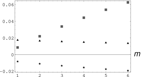
FIG. 1.: Coefficients of $\epsilon^{2}$ terms of the exponents $\eta_{l2}$ (triangles), $\eta_{l4}$ (stars), and $\beta_{q}$ (squares) for $n=1$.

In the special cases $m=2$ and $m=6$, the functions $\Phi(\upsilon;m,d^{*})$ and $\Xi(\upsilon;m,d^{*})$ become sufficiently simple [see (A6)–(A8)], so that the required integrations can be done analytically. This leads to

$$b_{\phi}(2)=-{1\over 54}{1\over(4\pi)^{8}}\;,$$ (133)

$$\check{b}_{\sigma}(2)={1\over 162}{1\over(4\pi)^{8}}\;,$$ (134)

$$\check{b}_{\rho}(2)={1\over 18}{1\over(4\pi)^{8}}\;,$$ (135)

$$b_{\phi}(6)=-{16\over 9}\,\frac{1-3\ln\!{\frac{4}{3}}}{(4\pi)^{12}}\;,$$ (137)

$$\check{b}_{\sigma}(6)={14\over 81}{1\over(4\pi)^{12}}\;,$$ (138)

and

$$\check{b}_{\rho}(6)={8\over 9}\,\frac{1+6\ln\!{\frac{4}{3}}}{(4\pi)^{12}}\;.$$ (139)

If these analytical expressions for the coefficients are inserted into the expansions (118), (121), and (127) of $\eta_{l2}$, $\eta_{l4}$, and $\beta_{q}$ with $m=2$ and $m=6$, then Sak and Grest’s[27] results for those two values of $m$ are recovered (which in turn agree with Mergulhão and Carneiro’s[32] findings for $\eta_{l2}$ and $\eta_{l4}$).

As was mentioned already in the Introduction, these results for $m=2$ and $m=6$ disagree with Mukamel’s[25]. More generally, our ${\mathcal{O}}(\epsilon^{2})$ results (115)–(127), for all values of $m=1,\ldots,6$, turn out to be at variance with the latter author’s. The case $m=1$ was also studied by Hornreich and Bruce[26], who calculated $\eta_{l4}(m{=}1)$ and $\beta_{q}(m{=}1)$ to order $\epsilon^{2}$. Their results agree with Mukamel’s and hence diagree with our’s.

Upon extrapolating the series expansions (115)–(127) one can obtain exponents estimates for three-dimensional systems. Unfortunately, there exist in the literature only very few predictions of exponent values produced by other means with which we can compare our’s.[6] Utilizing high-temperature series techniques, Redner and Stanley[36] found the estimate $\beta_{q}=0.5\pm 0.15$ for the case of a uniaxial $(m,d,n)=(1,3,1)$ Lifshitz point. This is in conformity with the value $\beta_{q}\simeq 0.519$ one gets by setting $\epsilon=1.5$ in the corresponding $m{=}1$ result of (127). A more recent high-temperature series analysis by Mo and Ferer[37] yielded $2\,\beta_{q}\simeq 1$. For the susceptibility exponent

$$\gamma_{l}=\nu_{l2}(2-\eta_{l2})=\nu_{l4}(4-\eta_{l4})\>,$$ (140)

the correlation exponent $\nu_{l4}$, and the specific-heat exponent

$$\alpha_{l}=2-m\,\nu_{l4}-(d-m)\,\nu_{l2}$$ (141)

of the $(m,d,n){=}(1,3,1)$ Lifshitz point these authors obtained the results $\gamma_{l}=1.62\pm 0.12$, $4\,\nu_{l4}=1.63\pm 0.10$, and $\alpha_{l}=0.20\pm 0.15$. Utilizing these numbers to compute $\eta_{l4}$ via the scaling law implied by (140), $\eta_{l4}=4-\gamma_{l}/\nu_{l4}$, yields $\eta_{l4}\simeq 0.02\pm 0.5$. This may be be compared with the value $\eta_{l4}\simeq-0.019$ one finds from (121) upon setting $\epsilon=1.5$.

As a further quantity for which Mo and Ferer’s results[37] yield an estimate that can be compared with our ${\mathcal{O}}(\epsilon^{2})$ results we consider the ratio $\beta_{l}/\gamma_{l}$. Substituting their exponent values into $\beta_{l}=(2-\alpha_{l}-\gamma_{l})/2$ yields $\beta_{l}=0.09\pm 0.135$ and $\beta_{l}/\gamma_{l}=0.055^{\,-\,0.081}_{\,+\,0.094}$. From the asymptotic form (25) of $G^{(N{=}1)}_{\mathrm{r}en}$ one reads off the scaling law

$$\beta_{l}=\frac{\nu_{l2}}{2}\left(d-m-2+\eta_{l2}\right)+\frac{\nu_{l4}}{2}\,m\;,$$ (142)

which may be combined with relation (140) for $\gamma_{l}$ to conclude that

$$\frac{\beta_{l}}{\gamma_{l}}={d-m-2+\eta_{l2}+m\,\frac{\nu_{l4}}{\nu_{l2}}\over 2\,(2-\eta_{l2})}\;.$$ (143)

We now set $m=n=1$ and $\epsilon=1.5$ in (115) and (118). This gives $\nu_{l4}/\nu_{l2}\simeq 0.488$ and $\eta_{l2}\simeq 0.039$. Then we insert these numbers into (143) with $d=3$, obtaining ${\beta_{l}}/{\gamma_{l}}\simeq 0.134$.

There also exist Monte Carlo estimates of exponents for the case of a $(m,d,n){=}(1,3,1)$ Lifshitz point.[38, 39] The more recent ones, $\beta_{l}=0.19\pm 0.02$ and $\gamma_{l}=1.4\pm 0.06$, due to Kaski and Selke[39], give ${\beta_{l}}/{\gamma_{l}}=0.136\pm 0.02$. In view of the fact that the importance of anisotropic scaling and its implications for finite-size effects in systems exhibiting anisotropic scale invariance[40, 41] has been realized only more recently, it is not clear to us how reliable these Monte Carlo estimates may be expected to be. Note, on the other hand, that the coefficients of the $\epsilon^{2}$ terms of the series (115)–(127) are all truly small. Thus it is not unlikely that the values one gets for $d=3$ by naive evaluation of these truncated series are fairly precise, at least for $m=1$. (The $\epsilon^{2}$-corrections of these exponents grow with $m$ because of the factor $(d^{*}-3)^{2}=(1+\frac{m}{2})^{2}$.)

V Concluding remarks

We have studied the critical behavior of $d$-dimensional systems at $m$-axial Lifshitz points by means of an $\epsilon$ expansion about the upper critical dimension $d^{*}=4+{m\over 2}$. Using modern field-theory techniques, we have been able to compute the correlation exponents $\eta_{l2}$ and $\eta_{l4}$, the wave-vector exponent $\beta_{q}$, and exponents related to these via scaling laws to order $\epsilon^{2}$. The resulting series expansions, given in (115)–(127), correct earlier results by Mukamel[25] and Hornreich and Bruce[26]; for the special values $m=2$ and $m=6$, we recovered Sak and Grest’s[27] findings.

To clarify this long-standing controversy, it proved useful to work directly in position space and to compute the Laurent expansion of the dimensionally regularized distributions associated with the Feynman diagrams. There are two other classes of difficult problems where this technique has demonstrated its potential: field theories of polymerized (tethered) membranes[42, 43, 44] and critical behavior in systems with boundaries.[34, 45] In the present study an additional complication had to be mastered: The free propagator at the Lifshitz point, which because of anisotropic scale invariance is a generalized homogeneous function rather than a simple power of the distance $|\boldsymbol{x}-\boldsymbol{x}^{\prime}|$, involves a complicated scaling function. For powers and products of simple homogeneous functions, a lot of mathematical knowledge on Laurent expansions is available.[33] Unfortunately, the amount of explicit mathematical results on Laurent expansions of powers and products of generalized homogeneous functions appears to be rather scarce. Since we had no such general mathematical results at our disposal, we had to work out the Laurent expansions of the required distributions by our own tools.

Difficulties of the kind we were faced with in the present work may be encountered also in studies of other types of systems with anisotropic scale invariance. Hence the techniques utilized above should be equally useful for field-theory analyses of such problems.

A The scaling functions $\Phi(\upsilon)$ and $\Xi(\upsilon)$

The scaling functions $\Phi(\upsilon)$ and $\Xi(\upsilon)$ introduced respectively through (25)–(26) and (50)–(51) are given by single integrals (28) and (52) of the form

$$i(\upsilon)=\upsilon^{-\mu}\int\limits_{0}^{\infty}dq\,q^{2-\epsilon}{\mathrm{J}}_{\mu}(q\upsilon){\mathrm{K}}_{\nu}(q^{2})\;.$$ (A1)

This is a standard integral,[46] which for arbitrary values of its parameters $\mu$ and $\nu$, can be expressed in terms of generalized hypergeometric functions ${{{}_{2\!}F_{3}}}$. For the special values $\mu={m\over 2}-1$ and $\nu=1-{m\over 4}-{\epsilon\over 2}$ or $\nu=-{m\over 4}-{\epsilon\over 2}$ for which it is needed, it simplifies, giving

$$\Phi(\upsilon;m,d)={1\over 2^{2+m}\,\pi^{\frac{6+m-2\,\epsilon}{4}}}\left[{\Gamma\big{(}1{-}{\epsilon\over 2}\big{)}\over\Gamma\big{(}{2{+}m\over 4}\big{)}}\,{{{}_{1\!}{\mathrm{F}}_{2}}}\!\left(1{-}{\epsilon\over 2};{1\over 2},{2{+}m\over 4};{\upsilon^{4}\over 64}\right)-{\upsilon^{2}\over 4}{\Gamma\big{(}{3\over 2}{-}{\epsilon\over 2}\big{)}\over\Gamma\big{(}1{+}{m\over 4}\big{)}}\,{{{}_{1\!}{\mathrm{F}}_{2}}}\!\left({3\over 2}{-}{\epsilon\over 2};{3\over 2},1{+}{m\over 4};{\upsilon^{4}\over 64}\right)\right]$$ (A2)

and

$$\Xi(\upsilon;m,d)={1\over 2^{3+m}\,\pi^{\frac{6+m-2\,\epsilon}{4}}}\left[{\Gamma\big{(}{1{-}\epsilon\over 2}\big{)}\over\Gamma\big{(}{m\over 4}\big{)}}\,{{{}_{1\!}{\mathrm{F}}_{2}}}\!\left({1{-}\epsilon\over 2};{1\over 2},{m\over 4};{\upsilon^{4}\over 64}\right)-{\upsilon^{2}\over 4}{\Gamma\big{(}1{-}{\epsilon\over 2}\big{)}\over\Gamma\big{(}{2{+}m\over 4}\big{)}}\,{{{}_{1\!}{\mathrm{F}}_{2}}}\!\left(1{-}{\epsilon\over 2};{3\over 2},{2{+}m\over 4};{\upsilon^{4}\over 64}\right)\right]\,.$$ (A3)

At the upper critical dimension, i.e., for $\epsilon=0$, this becomes

$$\Phi\!\Big{(}\upsilon;m,4{+}\frac{m}{2}\Big{)}=\frac{1}{2^{5+m}\,\pi^{\frac{6{+}m}{4}}}\left[{8\over\Gamma\big{(}{2{+}m\over 4}\big{)}}\;{{{}_{1\!}{\mathrm{F}}_{2}}}\!\left(1;{1\over 2},{2{+}m\over 4};{\upsilon^{4}\over 64}\right)-{2^{3m\over 4}\,\sqrt{\pi}}\,\upsilon^{2-{m\over 2}}\,{\mathrm{I}}_{m\over 4}\!\Big{(}{\upsilon^{2}\over 4}\Big{)}\right]$$ (A4)

and

$$\Xi\!\Big{(}\upsilon;m,4{+}\frac{m}{2}\Big{)}=\frac{1}{2^{6+m}\,\pi^{\frac{6{+}m}{4}}}\left[2^{3m\over 4}\,\sqrt{\pi}\,\upsilon^{2{-}{m\over 2}}\,{\mathrm{I}}_{{m\over 4}{-}1}\!\Big{(}{\upsilon^{2}\over 4}\Big{)}-\frac{2\,\upsilon^{2}}{\Gamma\big{(}{2{+}m\over 4}\big{)}}\,{{{}_{1\!}{\mathrm{F}}_{2}}}\!\left(1;{3\over 2},{2{+}m\over 4};{\upsilon^{4}\over 64}\right)\right]\;,$$ (A5)

respectively, where the ${\mathrm{I}}_{\nu}(.)$ are modified Bessel functions of the first kind.

In the special cases $m=2$ and $m=6$, these expressions reduce to simple elementary functions: One has

$$\Phi(\upsilon;2,5)={1\over(4\pi)^{2}}\,{\mathrm{e}}^{-{\upsilon^{2}\over 4}}\;,$$ (A6)

$$\Xi(\upsilon;2,5)={1\over 2}\,\Phi(\upsilon;2,5)\,,$$ (A7)

$$\Phi(\upsilon;6,7)={1-(1+{\upsilon^{2}\over 4})\,{\mathrm{e}}^{-{\upsilon^{2}\over 4}}\over(2\pi)^{3}\,\upsilon^{4}}\;,$$ (A8)

and

$$\Xi(\upsilon;6,7)={1\over(4\pi)^{3}}\,{1\over\upsilon^{2}}\left(1-{\mathrm{e}}^{-{\upsilon^{2}\over 4}}\right)\;.$$ (A9)

The reason for the latter simplifications is the following. If $m=2$ or $m=6$ and $d=d^{*}=4+m/2$ (upper critical dimension), then Bessel functions ${\mathrm{K}}_{\nu}$ with $\nu=\pm\frac{1}{2}$ are encountered in the integral (A1), which are simple exponentials.[47] This entails that the required single integrations can be done analytically to obtain the results (133)–(139) for the ${\mathcal{O}}(\epsilon^{2})$ coefficients.

For the remaining values of $m$, i.e., for $m=1,3,4,5$, the required integrals did not simplify to a degree that we were able to compute them analytically. However, proceeding as explained in Appendix B, they can be computed numerically. In the special cases $m=2$ and $m=6$, the results of our numerical integrations are in complete conformity with the analytical ones.

B Asymptotic behavior of the scaling functions $\Phi(\upsilon)$ and $\Xi(\upsilon)$

According to (A4), the scaling function $\Phi(\upsilon;m,d^{*})$ is a difference of a hypergeometric function ${{{}_{1\!}{\mathrm{F}}_{2}}}$ and a product of a Bessel function ${\mathrm{I}}_{m/4}$ times a power. If one asks Mathematica[48] to numerically evaluate expression (A4) for $\Phi(\upsilon)$ without taking any precautionary measures, the result becomes inaccurate whenever $\upsilon$ becomes sufficiently large. We found that such a direct, naive numerical evaluation fails for values of $\upsilon$ exceeding $\upsilon_{0}\simeq 9.5$. This is because both functions of this difference increase exponentially as $\upsilon\to\infty$.

To cope with this problem, we determined the asymptotic behavior of the scaling functions $\Phi(\upsilon;m,d^{*})$ and $\Xi(\upsilon;m,d^{*})$ for $\upsilon\to\infty$. From the integral representations (26) and (51) of these functions one easily derives the limiting forms

$$\Phi(\upsilon;m,d)\mathop{\approx}\limits_{\upsilon\to\infty}\Phi^{({\mathrm{a}s})}(\upsilon;m,d)\equiv\upsilon^{-4+2\epsilon}\,\Phi_{\infty}(m,d)$$ (B1)

and

$$\Xi(\upsilon;m,d)\mathop{\approx}\limits_{\upsilon\to\infty}\Xi^{({\mathrm{a}s})}(\upsilon;m,d)\equiv\upsilon^{-2+2\epsilon}\,{\Phi_{\infty}(m,d)\over 8\,(1-\epsilon)}\;,$$ (B2)

with

$$\Phi_{\infty}(m,d) = \int\limits_{\boldsymbol{q}_{\|}}\int\limits_{\boldsymbol{q}_{\perp}}\frac{{\mathrm{e}}^{i(\boldsymbol{q}_{\parallel}\cdot\boldsymbol{e}_{\parallel})}}{q_{\parallel}^{4}+q_{\perp}^{2}}$$ (B3)

$$= \frac{2^{2(d-m)-5}\,\pi^{\frac{1-d}{2}}\,\Gamma\big{(}d{-}2{-}\frac{m}{2}\big{)}}{\Gamma\big{(}\frac{3{-}d{+}m}{2}\big{)}}\;.$$ (B4)

At the upper critical dimension, the latter coefficient becomes

$$\Phi_{\infty}(m,d^{*})={2^{3-m}\,\pi^{-{6+m\over 4}}\,\over{\Gamma\big{(}{m-2\over 4}\big{)}}}\,.$$ (B5)

Note that for $m=2$ the asymptotic form (B1) is consistent with the simple exponential form (A6) since $\Phi_{\infty}(2,5)=0$. However, for other values of $m$, the coefficient (B5) does not vanish. For example, $\Phi_{\infty}(6,7)=1/(8\,\pi^{3})$, in conformity with expression (A8) for the scaling function $\Phi(\upsilon;6,7)$.

In order to obtain precise results for the integrals $J_{0,3}(m,d^{*})$, $J_{4,3}(m,d^{*})$, and $I_{1}(m,d^{*})$, on which the coefficients $b_{\phi}(m)$, $\check{b}_{\sigma}(m)$, and $\check{b}_{\rho}(m)$ depend, we proceeded as follows. We split the required integrals as $\int_{0}^{\infty}\ldots d\upsilon=\int_{0}^{\upsilon_{0}}\ldots d\upsilon+\int_{\upsilon_{0}}^{\infty}\ldots d\upsilon$, choosing $\upsilon\simeq 9.3$. In the integrals $\int_{\upsilon_{0}}^{\infty}\ldots d\upsilon$, we replaced the integrands by their asymptotic forms obtained upon substitution of $\Phi$ and/or $\Xi$ by their large-$\upsilon$ approximations $\Phi^{({\mathrm{a}s})}$ and $\Xi^{({\mathrm{a}s})}$ given in (B1) and (B2), respectively, and then computed these integrals analytically. The integrals $\int_{0}^{\upsilon_{0}}\ldots d\upsilon$ were computed numerically, using Mathematica.[48] We checked that reasonable changes of $\upsilon_{0}$ have negligible effects on the results. The procedure yields very accurate numerical values of the requested integrals. The reader may convince himself of the precision by comparing the so-determined numerical values of the integrals for $m=2$ and $m=6$ with the analytically known exact values.

REFERENCES

[1][‡]Permanent address.
[2][†] Permanent address:
Institute for
Condensed Matter Physics, 1 Svientsitskii str, 79011 Lviv, Ukraine
[3]
R. M. Hornreich, M. Luban, and S. Shtrikman, Phys. Rev. Lett. 35, 1678
(1975).
[4]
R. M. Hornreich, M. Luban, and S. Shtrikman, Phys. Lett. 55A, 269
(1975).
[5]
R. M. Hornreich, J. Magn. Magn. Mat. 15–18, 387 (1980).
[6]
W. Selke, in Phase Transitions and Critical Phenomena, edited by C. Domb
and J. L. Lebowitz (Academic Press, London, 1992), Vol. 15, pp. 1–72.
[7]
Y. Shapira, C. Becerra, N. O. Jr., and T. Chang, Phys. Rev. B 24, 2780
(1981).
[8]
For a more complete set of references, see Refs. [5] and
[6].
[9]
Y. M. Vysochanskiĭ and V. Y. Slivka, Usp. Fiz. Nauk 162, 139
(1992), [Sov. Phys. Usp. 35, 123–134].
[10]
E. Abraham and I. E. Dzyaloshinskii, Solid State Commun. 23, 883
(1977).
[11]
C. Hartzstein, V. Zevin, and M. Weger, J. Phys. (France) I 41, 677
(1980).
[12]
J. H. Chen and T. C. Lubensky, Phys. Rev. A 14, 1202 (1976).
[13]
A. Aharony and D. Mukamel, J. Phys. C 13, L255 (1980).
[14]
J. Lajzerowicz and J. J. Niez, J. Phys. (Paris) Lett. 40, L165 (1979).
[15]
M. E. Fisher and W. Selke, Phys. Rev. Lett. 44, 1502 (1980).
[16]
M. E. Fisher and W. Selke, Phil. Trans. R. Soc. Lond. 302, 1 (1981).
[17]
G. Gumbs, Phys. Rev. B 33, 6500 (1986).
[18]
K. Binder and H. L. Frisch, Eur. Phys. J. 10, 71 (1999).
[19]
H. L. Frisch, J. C. Kimball, and K. Binder, J. Phys. C 12, 29 (2000).
[20]
B. I. Halperin and P. C. Hohenberg, Rev. Mod. Phys. 49, 435 (1977).
[21]
B. Schmittmann and R. K. P. Zia, Statistical Mechanics of Driven Diffusive
Systems, Vol. 17 of Phase Transitions and Critical Phenomena (Academic
Press, London, 1995), pp. 1–220.
[22]
J. Krug, Adv. Phys. 46, 139 (1997).
[23]
For example, in a recent investigation[24] of the question of whether
anisotropic scale invariance may lead to an even larger invariance group
(reminiscent of conformal or Schrödinger invariance) such systems were
explicitly considered.
[24]
M. Henkel, Phys. Rev. Lett. 78, 1940 (1997).
[25]
D. Mukamel, J. Phys. A 10, L249 (1977).
[26]
R. M. Hornreich and A. D. Bruce, J. Phys. A 11, 595 (1978).
[27]
J. Sak and G. S. Grest, Phys. Rev. B 17, 3602 (1978).
[28]
G. S. Grest and J. Sak, Phys. Rev. B 17, 3607 (1978).
[29]
J. F. Nicoll, G. F. Tuthill, T. S. Chang, and H. E. Stanley, Phys. Lett. A 58, 1 (1976).
[30]
A. A. Inayat-Hussain and M. J. Buckingham, Phys. Rev. A 41, 5394
(1990).
[31]
C. Mergulhão, Jr. and C. E. I. Carneiro, Phys. Rev. B 58, 6047
(1998).
[32]
C. Mergulhão, Jr. and C. E. I. Carneiro, Phys. Rev. B 59, 13954
(1999).
[33]
I. M. Gel’fand and G. E. Shilov, in Generalized Functions (Academic
Press, New York and London, 1964), Vol. 1, Chap. 3.9 and 4.6.
[34]
H. W. Diehl, in Phase Transitions and Critical Phenomena, edited by C.
Domb and J. L. Lebowitz (Academic Press, London, 1986), Vol. 10, pp. 75–267.
[35]
To see this within the present calculational scheme, note that
is nothing but the Fourier transform of
at zero momentum . Hence it is equal to the integral
over the square of the Fourier transform of
, which can be read off from the Fourier-integral
representation (27) of . Upon performing the required
angular integrations, one is left with a standard integral, which yields
(130).
[36]
S. Redner and H. E. Stanley, Phys. Rev. B 16, 4901 (1977).
[37]
Z. Mo and M. Ferer, Phys. Rev. B 43, 10890 (1991).
[38]
W. Selke, Z. Phys. 29, 133 (1978).
[39]
K. Kaski and W. Selke, Phys. Rev. B 31, 3128 (1985).
[40]
K. Binder and J.-S. Wang, J. Stat. Phys. 55, 87 (1989).
[41]
K.-t. Leung, Phys. Rev. Lett. 66, 453 (1991).
[42]
F. David, B. Duplantier, and E. Guitter, Phys. Rev. Lett 72, 311
(1994).
[43]
F. David, B. Duplantier, and E. Guitter, preprint cond-mat/9702136
(unpublished).
[44]
K. Wiese, Habilitationsschrift, U. Essen, 1999;
in Phase Transitions and Critical Phenomena, edited by C.
Domb and J. L. Lebowitz (Academic Press, London, 2000), Vol. 19.
[45]
H. W. Diehl, Int. J. Mod. Phys. B 11, 3503 (1997), preprint
cond-mat/9610143.
[46]
A. Prudnikov, Y. A. Brychkov, and O. I. Marichev, Integrals and Series
(Gordon and Breach, New York, 1986), Vol. 2, eq. 2.16.22.6.
[47]
Both Sak and Grest [27] as well as Mergulhão and Carneiro
[32] explicitly employed the simple form (A6) of the scaling
function in their computations. However, the latter authors [32] did
not take advantage of working with the simple function (A8) in the
case , performing complicated computations in the momentum
representation instead. Sak and Grest[27], on the other hand, did not
present any details of their calculation for the case .
[48]
Mathematica, version 3.0, a product of Wolfram Research.