[

Localization of acoustic waves in 1D random liquid media

Abstract

We study acoustic propagation in one dimensional water ducts containing many air-filled blocks. The acoustic band structures for the periodic arrangements of the blocks is calculated, whereas the transmission for various random configurations of the blocks is computed by the transfer matrix method. The results show that while all waves are localized for any given amount of disorders, there is no genuine scaling behavior for the system. The results also reveal a distinct collective behaviour for localized waves, a feature useful for distinguishing the localization from the residual absorption effect.
PACS numbers: 43.20., 71.55J, 03.40K

]

The fact that the electronic localization in disordered systems[1] is of wave nature has led to suggestion that classical waves could be similarly localized in random systems. The effort in searching for localization of classical waves such as acoustic and electro-magnetic waves is tremendous. It has drawn intensive attentions from both theorists [2, 3, 4, 5, 6, 7, 8, 9, 10] and experimentalists[11, 12].

Localization of waves in one dimensional (1D) systems has attracted particular interest from scientists because in higher dimensions the interaction between waves and scatterers is so complicated that the theoretical computation is rather involved and most solutions require a series of approximations which are not always justified, making it difficult to relate theoretical predictions to experimental observations. Yet wave localization in one dimension (1D) poses a more manageable problem which can be tackled in an exact manner by the transfer matrix method. Moreover, results from 1D can provide insight to the problem of wave localization in general and are suitable for testing various ideas. Indeed, over the past decades considerable progress has been made in understanding the localization behavior in 1D disordered systems[13]. However, a number of important issues remained untouched. These issues include, for example, how waves are localized inside the media and whether there is a distinct feature for wave localization which would allow to differentiate the localization from residual absorption effect without ambiguity[14, 15]. Results from the statistical analysis of the scaling behavior in 1D random media is not conclusive. A further question could be whether the localized state is a phase state which would accommodate a more systematic interpretation from the view of a symmetry breaking and collective behavior, in analogy to phase states such as superconductivity. This Letter attempts to provide insight to these questions.

Here we study the problem of acoustic wave propagation in one dimensional water ducts containing many air blocks either regularly or randomly but on average regularly distributed inside the ducts. The frequency band structures and wave transmission are computed numerically. We show that while our results affirm the previous claim that all waves are localized inside an 1D medium with any amount of disorder, there are, however, a few distinctive features in our results. Among them, in contrast to optical cases[17], there is no universal scaling behavior in the present system. In addition, when waves are localized, a collective behaviour of the system emerges.

Assume that $N$ air blocks of identical thickness $a$ are placed regularly or randomly in a water duct with length $L$ measured from the left boundary of the duct (LB). The air fraction is $\beta=Na/L$, the average distance between two adjacent water layers is $\langle d\rangle=L/N=a/\beta$, and the average thickness of water layers is $\langle b\rangle=(\sum^{N}_{j=1}b_{j})/N$. The degree of randomness for the system is controlled by a parameter $\Delta$ in such a way that the thickness of the $j$-th water layer is $b_{j}=\langle b\rangle(1+\delta_{j})$ with $\delta_{j}$ being a random number within the interval $[-\Delta,\Delta]$; the regular case corresponds to $\Delta=0$. An acoustic source placed at LB generates monochromatic waves with an oscillation $v(t)=ve^{-i\omega t}$. Transmitted waves propagate through the $N$ air layers and travel to the right infinity. In order to avoid unnecessary confusion, possible effects from surface tension, viscosity or any absorption are neglected. For convenience, we use the dimensionless quantity $k\langle b\rangle$ to measure the frequency, where $k=\omega/c$ is the wave number and $c$ is the sound speed in water. Similarly, $k_{g}$ and $c_{g}$ represent the wave number and sound speed in the air blocks respectively.

The wave propagation in such a system can be solved using the transfer matrix method[4]. After dropping out the time factor $e^{-i\omega t}$, the wave propagation is governed by two equations[16]. The first is the Helmholtz equation,

$$p_{m}^{\prime\prime}(x)+k^{2}_{m}p_{m}(x)=0,$$ (1)

in which $p_{m}(x)$ is the pressure field, and the subscript $m$ refers to the medium that can be either water or air, depending on where $x$ is located. Within any layer, Eq. (1) warrants two solutions: $A_{m}e^{ik_{m}x}$ represents the wave transmitted away from the source to the right and $B_{m}e^{-ik_{m}x}$ the wave reflected towards the source. The total wave is therefore $p_{m}(x)=A_{m}e^{ik_{m}x}+B_{m}e^{-ik_{m}x}$. The second equation relates the oscillation velocity and the pressure field,

$${u}_{m}(x)=\frac{1}{i\omega\rho_{m}}p^{\prime}_{m}(x)=(A_{m}e^{ik_{m}x}-B_{m}e^{-ik_{m}x})/\rho_{m}c_{m},$$ (2)

where $\rho_{m}$ refers to the equilibrium mass density of medium $m$.

The coefficients $A_{m}$ and $B_{m}$ in any two adjacent layers are connected by a transfer matrix. By invoking the condition that the pressure and velocity fields are continuous across the interfaces separating water and air and the condition that there is no reflected wave to the right end of the system, the matrix elements for the transfer matrices linking all interfaces can be deduced, and waves in any particular block is therefore completely determined. The ratio between the amplitude of the outgoing wave at the right boundary and that of the transmitted wave at the source defines the transmission rate.

Before going further, a general discussion on wave propagation is in place. When waves propagate through media alternated with different material compositions, multiple scattering of waves is established by an infinite recursive pattern of rescattering. In terms of wave fields, the energy flow in the system is calculated from $J\sim\mbox{Re}[i(p^{*}(x)\partial_{x}p(x)]$. Writing $p(x)=|A(x)|e^{i\theta(x)}$ with $|A|$ and $\theta$ being the amplitude and phase respectively, the energy flow becomes $J\sim|A|^{2}\partial_{x}{\theta}$. Obviously, the energy flow will come to a complete halt and the waves could be localized in space when phase $\theta$ is constant and $|A|$ does not equal zero.

First consider the case with the periodic placement of air blocks (with spatial period $d$, water layer thickness $b$). According to Bloch theorem, and the wave field $p$ can be written as

$$p(x)=A(x)e^{iKx},$$ (3)

where $A(x)$ is a periodic function satisfying $A(x+d)=A(x)$, and $K$ is the Bloch wave number represented in the dispersion relation

$$\cos Kd=\cos k_{g}a\,\cos kb-\cosh 2\eta\,\sin k_{g}a\,\sin kb.$$ (4)

Here $k_{g}=k/h$ and $\eta=\ln q$ with $q^{2}=gh$ and $g=\rho_{g}/\rho$, $h=c_{g}/c$.

The band structures for four air-fractions are shown in Fig. 1. The ranges covered by the dispersion curves refer to the passing bands, while the areas sandwiched by any two curves to the complete band gaps. Within the gap, waves are evanescent and cannot propagate. Since the air blocks are strong scatterers due to the large contrast in acoustic impedance between air and water, we see that even a small air-fraction can lead to wide band gaps as seen in Fig. 1(a). With increasing $\beta$, the passing bands are narrowed and become streaks. When the air-fraction is reduced, however, the band gaps gradually disappear, as shown by Fig. 1(d).

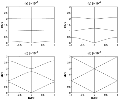
FIG. 1.: Band structures of an infinite periodic system for four different air fractions ($\beta$). In the plots, $K$ is the Bloch wave number and $d$ is the lattice spacing.

Wave propagation properties can be significantly affected by varying air-fraction or adding randomness. Fig. 2(a) presents the typical results of the transmission rate as a function of $k\langle b\rangle$ for various $\beta$ at a given randomness. At frequencies for which the wavelength is smaller than the averaged distance between air blocks, the transmission is significantly reduced by increasing air fraction.

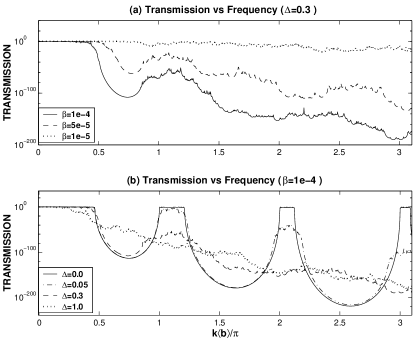
FIG. 2.: Transmission versus $k\langle b\rangle/\pi$ for various air fractions at $\Delta=0.3$ (a) and different disorders (b). The number of the air-blocks is 100.

Fig. 2(b) illustrates the effect of the randomness $\Delta$ on transmission for a given air-fraction. For comparison, the transmission in the corresponding regular array ($\Delta=0$) is also plotted. The gaps are located between $k\langle b\rangle/\pi=0.46$ and $1$, $1.21$ and $2$, $2.12$ and $3$, and so on. We find that for frequencies located inside the band gaps of the corresponding regular array, the disorder-induced localization effect competes yet reduces the band gap effect. To characterize wave localization in this case, both the band gap and the disorder effects should be considered, supporting the two parameter scaling theory[17]. However, increasing disorder tends to smear out the band structures. When exceeding a certain amount, the effect from the disorder suppresses the band gap effect completely, and there is no distinction between the localization at frequencies within and outside the band gaps.

Fig. 2 shows that the localization behaviour depends crucially on whether the wavelength ($\lambda$) is greater than the average distance between air blocks. When $\langle b\rangle/\lambda$ is less than one, the localization effect is weak. We also observe that with the added disorder, the transmission is enhanced in the middle of the gaps. Similar enhancement due to disorder has also been reported recently[19]. Differing from [19], however, the transmission at frequencies within the gaps of the corresponding periodic arrays in the present system is not always enhanced by disorder. Instead the transmission is reduced further by the disorder near the band edges.

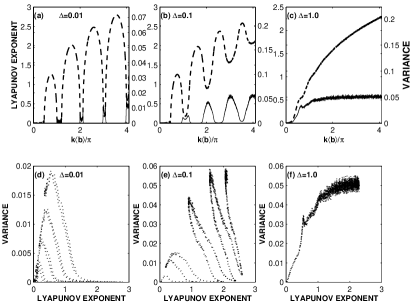
FIG. 3.: Diagrams (a), (b), and (c) show the Lyapunov exponent (LE) in broken lines and its variance in solid lines as a function of $k\langle b\rangle/\pi$. Diagrams (d), (e), and (f) present the plots of the exponent versus its variance. Here $\beta=10^{-4}$.

Fig. 3 presents the results for Lyapunov exponent (LE) and its variance as a function of non-dimensional frequency $k\langle b\rangle/\pi$. At low disorders, the variance of LE inside the gaps is small. Contrast to the optical case[17], there are no double maxima inside the gap. With increasing disorder, double peaks appears inside the allow bands. When exceeding a certain critical value, however, the double peaks emerge. The higher frequency, the lower is the critical value. For example, the double peaks are still visible in the first allow band (c. f. Fig. 3(b)), while there is only one peak inside the higher passing bands. Meanwhile, the increasing disorder reduces the band gap effect and smears LE, in accordance with Fig. 2. We also plot LE-variance relation in Fig. 3. With increasing disorder, we do not observe genuine linear dependence between LE and its variance, as expected from the single parameter scaling theory.

In the past the localization phenomenon in 1D is usually characterized by LE, here we propose to use a phase behavior of the waves to characterize the localization. We compute the energy density inside the sample from

$$E_{m}(x)=\frac{\rho_{m}}{4}\left(|u_{m}|^{2}+\frac{|p_{m}|^{2}}{\rho^{2}_{m}c^{2}_{m}}\right),$$ (5)

where $m$ refers to either water or air. Meanwhile, the phases of $p(x)$ and $u(x)$ are recorded. Expressing $p(x)$ and $u(x)$ as $A_{p}(x)e^{i\theta_{p}(x)}$ and $A_{u}(x)e^{i\theta_{u}(x)}$, we construct unit phase vectors $\vec{v}_{p}=\cos\theta_{p}\hat{e}_{x}+\sin\theta_{p}\hat{e}_{y}$ and $\vec{v}_{u}=\cos\theta_{u}\hat{e}_{x}+\sin\theta_{u}\hat{e}_{y}$. Then the behavior of the phase vectors along the path are investigated. Physically, these phase vectors represent the oscillation behavior of the system.

Typical results for the spatial distribution of the energy and the phase behaviour for the given disorder and air fraction are shown in Fig. 4. Here for the sake of convenience, only the phase vectors at the interfaces between air and water are shown. First, we note that the energy density is constant in each individual block. This is a special feature of 1D classical systems, and can be verified by a deduction from Eq. (5). We find that when the sample size is sufficiently large, waves are always localized for any given amount of randomness. When localized, the waves are trapped inside the medium, but not necessarily confined at the site of the source, unless the band gap effect is dominant. The energy distribution does not follow an exponential decay along the path. This differs from situations in higher dimensions[8, 20]. It is also shown that the energy stored in the medium can be tremendous (c. f. Figs. 4(a) and (b)). With increasing sample size, the peak amplitude may grow, pointing to the stochastic resonance, in agreement with [2]. When disorder is weak and for frequencies within the gaps, such a stochastic resonance behavior disappears.

It is also observed that for all frequencies, there is a collective behavior for the phase vectors. In Fig. 4(c) we plot the phase vectors in three spatial regimes, namely, near the transmitting site, in the middle of the duct, and at the far end from the source. Symbols $p^{L}$, $p^{R}$, $u^{L}$, $u^{R}$ appearing in Fig. 4(c) denote respectively the phase vectors for the pressure and the velocity fields on the left and right side of the air blocks. It is clear that when waves are localized, all the phase vectors of the pressure field are pointing to either $\pi/2$ or $-\pi/2$, and perpendicular to the phase vectors of the velocity field. The pressure at the two sides of any air block varies in phase. Mostly, the two sides also oscillate in phase. Different from higher dimensional cases in which all phase vectors of localized fields point to the same direction[9, 20], the present phase vectors are constant by domains; this ensures no energy flows. The velocity field in neighboring domains oscillate exactly out of phase. The phase vector domains are sensitive to the arrangement of the air blocks. We stress that such a phase ordering not only exists for the boundaries of the air blocks, but also appears inside the whole medium.

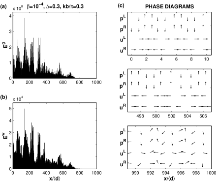
FIG. 4.: Energy distribution and phase diagrams for localized state. Here $\beta=10^{-4}$, $\Delta=0.3$ and $k\langle b\rangle=0.3\pi$ is a frequency in the first allowed band. (a) Energy densities in the air blocks. (b) Energy densities in water. (c) Phase vectors at the interfaces for three spatial ranges of the medium. The unit of energy density is $J/m^{3}$.

The coherence behavior is a unique feature for wave localization, which could be verified by the cross correlation measurement. At the far end of the sample, however, the phase vectors become gradually disoriented, implying that the energy can leak out only at the boundary due to the finite sample size. This boundary effect vanishes exponentially as the sample size is increased. The fact that the phase vectors are constant in domains indicates that once waves are localized, no more energy can be pumped into the system. When localization is evident, increasing the sample size by adding more air blocks will not change the patterns of the energy distribution and phase vectors. Therefore the energy localization and the phase behavior are not caused by the boundary effect.

In summary, we have demonstrated a phase transition in acoustic propagation in an 1D random liquid medium. The results have shown that waves are always confined in a finite spatial region. The disorder leads a significant energy storage in the system. It is also indicated that the wave localization is related to a collective behavior of the system in the presence of multiple scattering, also observed for higher dimensions[9, 20]. The appearance of such a collective phenomenon may be regarded as an indication of a kind of Goldstone modes in the context of the field theory[21].

The work received support from National Science Council (No. NSC89-2611-M008-002 and NSC89-2112-M008-008).

REFERENCES

- [1] P. W. Anderson, Phys. Rev. 109, 1492 (1958).
- [2] U. Frisch, C. Froeschle, J. P. Scheidecker, and P. L. Sulem, Phys. Rev. A 8, 1416 (1973).
- [3] C. H. Hodges, J. Sound and Vibration, 82, 411 (1983).
- [4] V. Baluni and Willemsen, Phys. Rev. A 31, 3358 (1985).
- [5] C. M. Soukoulis, E. N. Economou, G. S. Grest and M. H. Cohen, Phys. Rev. Lett. 62, 575 (1989).
- [6] D. Sornette and O. Legrand, J. Acoust. Soc. Am. 92 (1992).
- [7] A. R. McGurn, K. T. Christensen, F. M. Mueller, and A. A. Maradudin, Phys. Rev. B 47, 13120 (1993).
- [8] Z. Ye and A. Alvarez, Phys. Rev. Lett. 80, 3503 (1998).
- [9] Z. Ye, H. Hsu, E. Hoskinson, and A. Alvarez, Chin. J. Phys. 37, 343 (1999).
- [10] M. Asch, W. Kohler, G. Papanicolaou, M. Postel, and B. White, SIAM Review 33, 519-625 (1991).
- [11] C. H. Hodges and J. Woodhouse, J. Acoust. Soc. Am. 74, 894 (1983).
- [12] R. Dalichaouch, J. P. Armstrong, S. Schultz, P. M. Platzman and S. L. McCall, Nature, 354, 53 (1991).
- [13] I. M. Lifshits, S. A. Gredeskul, L. A. Pastur, Introduction to the Theory of Disordered Systems. (A Wiley-Interscience Publication, New York, 1988).
- [14] F. Scheffold, R. Lenke, R. Tweer and G. Maret, Nature, 398, 206 (1999).
- [15] A. A. Chabanov, M. Stoytchev and A. Z. Genack, Nature, 404, 850 (2000).
- [16] A. Ishimaru, Wave Propagation and Scattering in Random Media. (Academic, New York, 1978).
- [17] L. I. Deych, D. Zaslavsky and A. A. Lisyansky, Phys. Rev. Lett. 81, 5390 (1998).
- [18] P. W. Anderson, D. J. Thouless, E. Abrahams, and D. S. Fisher, Phys. Rev. B 22, 2519 (1980).
- [19] V. D. Freilikher, B. A. Liansky, I. V. Yurkevich, A. A. Maradudin, and A. R. McGurn, Phys. Rev. E 51, 6301, (1995).
- [20] E. Hoskinson and Z. Ye, Phys. Rev. Lett. 83, 2734 (1999).
- [21] H. Umezawa, Advanced Field Theory, (AIP, New York, 1995).