Exact sampling from non-attractive distributions using summary states

Abstract

Propp and Wilson’s method of coupling from the past allows one to efficiently generate exact samples from attractive statistical distributions (e.g., the ferromagnetic Ising model). This method may be generalized to non-attractive distributions by the use of summary states, as first described by Huber. Using this method, we present exact samples from a frustrated antiferromagnetic triangular Ising model and the antiferromagnetic $q=3$ Potts model. We discuss the advantages and limitations of the method of summary states for practical sampling, paying particular attention to the slowing down of the algorithm at low temperature. In particular, we show that such a slowing down can occur in the absence of a physical phase transition.

I Introduction

In many statistical problems, physical and otherwise, it is useful to be able draw samples from a complex distribution. For example, in statistical physics one is interested in the Boltzmann distribution

$$P(\sigma)={e^{-\beta E(\sigma)}\over Z}\,,$$ (1)

where $E(\sigma)$ describes the energy of a system in configuration $\sigma$, $\beta$ is the inverse temperature (we set $k_{B}=1$), and $Z$ is a normalizing constant (the partition function). In general, $E(\sigma)$ may be easy to evaluate for a particular configuration, but the number of possible configurations makes it impractical to draw directly from the distribution. Yet some efficient method of sampling is desirable, as this would allow one to calculate properties of the system that might not be easily computed by analytical means.

In traditional Monte Carlo sampling methods, such as the Metropolis-Hastings method [1] and Gibbs sampling [2] (also known as the heat bath algorithm), one constructs an ergodic Markov chain whose stationary distribution is the desired distribution. By starting in some state and evolving the chain for a sufficiently long time, one can approximate a sample from the desired distribution. Unfortunately, such a sample is exact only in the limit of infinite time. In practice, it is often difficult to determine how long to wait to achieve sufficiently good samples, and one inevitably either produces poor samples or wastes time by running the Markov chain for longer than necessary.

However, in 1996, Propp and Wilson demonstrated the possibility of exact sampling by the method of coupling from the past, allowing one to produce perfect samples in a finite number of steps [3]. In the most general case, their method requires the infeasible task of running a Markov chain for every possible initial state of the system. But for certain distributions, termed attractive (such as a ferromagnetic Ising model), Propp and Wilson showed that the task may be greatly simplified by tracking only extremal states, permitting the practical calculation of exact samples. This method was generalized to anti-attractive distributions by Häggström and Nelander [4]. More recently, Huber showed that one may instead track only a single state that summarizes one’s knowledge of the system [5]. Because it does not require that the states be partially ordered, this last method is applicable to non-attractive distributions.

Using the summary state method, we have drawn exact samples from the antiferromagnetic triangular Ising model and from the Potts model. Fig. 1 shows one such sample. In §II, we describe the methods that make this possible. In §III, we briefly discuss the Ising and Potts models. We present results from the exact sampling of these models in §IV. Finally, we discuss the convergence properties of the summary state method, and we suggest practical generalizations.

FIG. 1.: An exact sample from a triangular Ising antiferromagnet with 14,400 spins at $\beta^{-1}=4.9$ and zero applied magnetic field.

II Coupling from the past and the summary state method

Propp and Wilson’s method of coupling from the past [3] is based on the observation that, for a fixed choice of the random numbers used to propagate a Markov chain, its possible paths in state space may ultimately coalesce into a single trajectory. Once two initial states lead to the same state, they will remain in lock step thereafter.

Consider simulating a Markov chain from every possible initial state at some fixed time $t=-T$, with the goal of taking a sample at $t=0$. If all the chains coalesce before $t=0$, then this finite procedure yields the same results as a Monte Carlo simulation started at an infinite time in the past, so the result is an exact sample. If the chains fail to coalesce, one can simply double the starting time to $-2T$, reusing the random numbers for the interval $[-t,0]$ (i.e., treating the random numbers as a function of simulation time), and repeat until coalescence is achieved.

Having to follow every possible state would make this method exponentially intractable. But for problems that admit a partial ordering of the states and which are “attractive” — that is, which preserve the ordering under evolution of the Markov chain — the computation can be vastly simplified by tracking only the extremal states. An example of an attractive system is the ferromagnetic Ising model, in which it is energetically favorable for spins to align with each other.

Huber [5] and Harvey and Neal [6] have shown that the method of Propp and Wilson may be generalized using a single summary state instead of a pair of extremal states. This single state summarizes one’s knowledge of the possible states of the system, allowing the state of some subsystems to be uncertain.

For example, suppose the system is a collection of variables $\sigma_{i}$ taking on the values $\{\pm 1\}$. Conventional Gibbs updating sets

$$\sigma_{i}\mapsto\left\{\matrix{+1&{\rm if\ }u\leq P(\sigma_{i}=+1|\bar{\sigma}_{i})\cr-1&{\rm if\ }u>P(\sigma_{i}=-1|\bar{\sigma}_{i})}\right.\,,$$ (2)

where $u$ is uniformly distributed on $[0,1]$ and $\bar{\sigma}_{i}$ denotes the set of all variables but the $i$th. To implement summary states, we allow each variable to take on the additional value ? which indicates uncertainty. We then run a modified Markov chain on this system: $\sigma_{i}$ is updated according to Eq. (2) if the result is the same for any possible assignment of $\pm 1$ to the ?’s in $\bar{\sigma}_{i}$; otherwise, $\sigma_{i}\mapsto\mbox{\tt?}$. As in the Propp and Wilson method, we run the chain from successively longer times in the past with random numbers as a function of simulation time. When no variables remain in ? states, the algorithm has converged, and we may take a sample at $t=0$.

For the case of attractive distributions, this procedure is exactly equivalent to the Propp and Wilson scheme. The value ? denotes variables that differ between the maximal and minimal states, and removal of all ? states corresponds to coalescence of the bounding chains. However, using a single summary state, there is no requirement that the states be ordered in any way. Thus the summary state method can also be applied to non-attractive distributions — for example, the antiferromagnetic Ising model.

Although the samples returned by this method are exact, the algorithm does not necessarily converge after a reasonable amount of time. Huber has shown that for antiferromagnetic spin systems at sufficiently high temperature, the expected running time of the algorithm is polynomial in the number of spins [5]. However, for systems with a phase transition, the convergence time diverges as a power law at the critical temperature, a phenomenon known as critical slowing down [7].

III The Ising and Potts models

Consider the Hamiltonian

$$E(\sigma)=-{1\over 2}\sum_{m,n}J_{mn}\sigma_{m}\sigma_{n}-\sum_{m}H_{m}\sigma_{m}\,,$$ (3)

where $J_{mn}$ is the coupling between spins $m$ and $n$ and $H_{m}$ is the value of an external magnetic field at the location of spin $m$. The appropriate Markov chain update rule is Eq. (2) with

$$P(\sigma_{i}=\pm 1|\bar{\sigma}_{i})={e^{-\beta E(\sigma_{i}=\pm 1)}\over e^{-\beta E(\sigma_{i}=+1)}+e^{-\beta E(\sigma_{i}=-1)}}\,.$$ (4)

In the Ising model [8], $J_{mn}$ is taken to be zero unless spins $m$ and $n$ are adjacent, in which case it is some constant $J$. Cases of particular interest are the square lattice, in which each spin has four neighbors, and the triangular lattice, with six neighbors per spin. In general, the behavior of Ising systems can vary with their spin connectivity. For both kinds of lattices, we use periodic boundary conditions. Because we may simultaneously update the states of spins whose conditional distributions are independent, one iteration of the Markov chain consists of two sweeps for the square lattice and three for the triangular lattice.

In this paper, we use the normalization $J=\pm 1$. $J=+1$ corresponds to the ferromagnetic case, in which spins prefer to point in the same direction; $J=-1$ corresponds to the antiferromagnet. As mentioned previously, the ferromagnetic case is attractive. The antiferromagnet on a square lattice is a special case, because its properties are isomorphic to those of a square ferromagnet. However, for a triangular lattice, there is no such isomorphism. With six neighbors per spin, there is no way to minimize the energy locally at all sites: we say the system is frustrated.

It is well known that a two-dimensional ferromagnetic Ising model exhibits a phase transition [9]. Below a critical temperature $\beta_{c}^{-1}$, there is spontaneous symmetry breaking, and the system develops a preferred spin orientation in the absence of any magnetic field. For a square lattice, $\beta_{c}^{-1}=2.27$. At this temperature, the relaxation time of the dynamic system diverges, a phenomenon known as critical slowing down [7]. Correspondingly, there is a divergence in the convergence time for some Markov chain Monte Carlo algorithms, such as coupling from the past, and exact samples cannot be generated for lower temperatures. Note that there is no phase transition in the case of a triangular antiferromagnet [10], so there cannot be a critical slowing down in the traditional sense.

To circumvent the problem of nonconvergence below the critical temperature, Propp and Wilson actually used a related system, the random cluster model, to generate Ising samples [3]. Unfortunately, this model has no obvious analog in the antiferromagnetic case.

The Potts model is a generalization of the Ising model wherein spins may take on $q$ different values $\{0,1,\ldots,q-1\}$ [11, 12]. Spins interact only with others of the same type. The Hamiltonian is

$$E(\sigma)=-{1\over 2}\sum_{m,n}J_{mn}\delta_{\sigma_{m},\sigma_{n}}-\sum_{m,k}H_{m}^{k}\delta_{\sigma_{m},k}\,.$$ (5)

Specifically, we consider the antiferromagnetic Potts model with $q=3$ on a square lattice with zero magnetic field. This model has a critical point only at $\beta^{-1}=0$, so there is no phase transition [13].

IV Results

A Ising model

By implementing the summary state method, we have produced exact samples from the Ising and Potts models. For example, Fig. 1 shows a sample from a triangular Ising antiferromagnet consisting of $120^{2}=14,400$ spins at $\beta^{-1}=4.9$ with zero applied magnetic field.

We find that the number of iterations required for the algorithm to converge diverges at a threshold temperature. We have studied this divergence using a lattice of $N=63^{2}=3969$ spins. Simulations using larger $N$ (e.g., $N=99^{2}$) suggest that the outcome is not significantly affected by choosing a larger grid size. Fig. 2 shows the divergence, to which we have fitted a power law of the form

$$t={a\over(\beta^{-1}-\beta^{-1}_{t})^{b}}+c\,.$$ (6)

We find that the time diverges with an exponent $b=1.03\pm 0.01$ at the threshold temperature $\beta^{-1}_{t}=4.839\pm 0.005$.

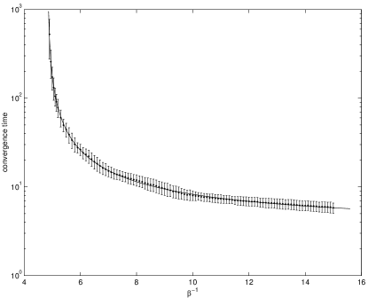
FIG. 2.: Variation with temperature of the number of iterations required for convergence of the summary state algorithm for the triangular, antiferromagnetic Ising model. Each point corresponds to either 500, 1000, or 1500 exact samples, with more samples taken at lower temperature. The solid line shows the fit to Eq. (6).

This divergence is an important feature of the summary state method. It is qualitatively similar to critical slowing down, but note that no physical phase transition is involved. In divergent situations the augmented Markov chain has a metastable set of distributions with many ?’s, such that it is very unlikely for it to enter a state with no ?’s.

To draw an exact sample using the summary state method, the system must go from a completely uncertain state to a completely certain state. Thus, it must pass through a state with only a few scattered ?’s. For temperatures sufficientlty near the threshold, where we know that such a sparse configuration can be reached, we might expect that the limiting factor is the probability that an isolated ? can cause divergence.

Therefore, as a very rough estimate, we might suppose that the divergence occurs when the probability of a single ? turning one of its six neighbors into a ? rises above $1\over 6$. We expect that the neighbors of any given spin $\sigma_{i}$ should be (on average) half up and half down. Replacing one of these neighbors by a ?, we may assume the configuration $(\uparrow\uparrow\uparrow\downarrow\downarrow\mbox{\tt?})$ without loss of generality. Then the threshold temperature is determined by

$$1-{1\over 1+e^{4\beta}}-{1\over 2}={1\over 6}\,,$$ (7)

which has the solution $\beta^{-1}=4/\ln 2\approx 5.8$.

To examine the validity of a threshold temperature analysis based on the persistence of single ?’s, we compiled statistics on the stability of an equilibrium system with a single ? added. Because we cannot create exact samples for much of the temperature range of interest, we generated approximate samples by simulating for fixed time (100 iterations) a random initial state. We then set one spin to ? and simulated the system forward. If any uncertainty remained after 500 iterations, we said the system diverged. Fig. 3 shows the fraction of divergent trials for various temperatures. As one would expect, this fraction goes to zero very near the threshold temperature.

FIG. 3.: Fraction of equilibrium systems that diverged after a single ? was added. The data are from 9000 trials at each temperature.

It is also interesting to consider how the algorithm behaves when a uniform nonzero magnetic field $H$ is applied. Biasing the spins makes it easier for them to choose a particular orientation, so we would expect convergence to be easier. Fig. 4 shows the region of convergence in the $(\beta^{-1},H)$ plane.

FIG. 4.: Region of convergence for the summary state algorithm on the triangular antiferromagnetic Ising model. Points in region (1) allow convergence, whereas points in region (2) are inaccessible to the algorithm. Each data point corresponds to 45 searches for the threshold, each using a different set of random numbers.

B Potts model

In addition, we have implemented exact sampling of the Potts model for arbitrary $q$. Fig. 5 shows an exact sample with $q=3$ for a square antiferromagnetic lattice of $100^{2}=10,000$ spins.

FIG. 5.: An exact sample from the $q=3$ antiferromagnetic Potts model for a 10,000 spin square lattice at $\beta^{-1}=1.2$.

A naïve implementation of the summary state method would augment the possible spin values with a single ?. We refer to this method as algorithm $A$. However, it is possible to retain more information about uncertain spins: for each spin, we store a binary $q$-bit vector $(b_{1},b_{2},\ldots,b_{q})$, $b_{i}\in\{0,1\}$. Bit $b_{i}$ is set to one if it is possible for the spin to take on the value $i$: thus the initial state of each spin is $b=(1,1,\ldots,1)$. In updating the state of the system, we set $b_{i}=0$ only when the spin cannot take on the value $i$ for any allowed configuration of its neighbors. We refer to the latter method as algorithm $B$.

To demonstrate the advantage of retaining more information in the summary state, we have studied the convergence properties of both algorithms. This comparison is shown in Fig. 6, based on data for a square $64^{2}=4096$ spin lattice. As in the Ising study, both algorithms lead to a power law divergence with an exponent of one ($b_{A}=1.04\pm 0.03$, $b_{B}=0.99\pm 0.02$). However, the threshold temperatures for the two algorithms are quite different: $\beta^{-1}_{t,A}=2.293\pm 0.005$, whereas $\beta^{-1}_{t,B}=1.157\pm 0.004$. As in the Ising example above, neither of the divergences corresponds to a physical phase transition.

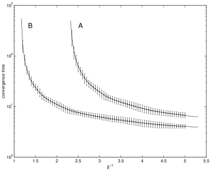
FIG. 6.: Temperature dependence of the convergence time for the square, antiferromagnetic $q=3$ Potts model under algorithms $A$ and $B$. Each point corresponds to 1600 exact samples on a 4096 spin lattice. The solid lines give fits to Eq. (6).

V Conclusions

We have demonstrated the usefulness of the summary state method for exact sampling from non-attractive distributions. In both the antiferromagnetic Ising and Potts models, the method works above a certain threshold temperature, with a power law divergence in the coalescence time at the threshold. Although similar to the phenomenon of critical slowing down, this divergence does not occur at a physical phase transition. As the Potts example shows, the location of the divergence is a feature of the specific implementation of the summary states, not of the underlying distribution. We have shown that retaining more information in the summary state will allow convergence at lower temperatures.

Based on this result, we may propose an improved algorithm for the triangular antiferromagnetic Ising model. At lower temperatures, the system should be increasingly ordered, and tracking this order might make it easier to gain incremental knowledge of the state of the system. One idea is to keep track of correlations between spins by grouping them into hexagonal clumps of seven, which can be used to tile the triangular lattice. Each tile has $2^{7}=128$ possible states. In analogy to the Potts method presented earlier (in which a $q$-bit vector represents the uncertainty about a spin), representing each tile with a 128-bit vector would allow individually tracking the possible arrangements of those seven spins. Within a tile, the summary state can track anticorrelation, which we expect to arise at low temperatures. Each edge of a tile can be easily summarized in a 4-bit vector for comparison with its neighboring tiles. Each tile can then update its summary state by considering the possible states of the neighboring edges.

Of course, summary state sampling remains a valuable tool even if it cannot be done below some threshold. Where it does work, it is exact. The method also has the advantage that we need not even know if the distribution in question is attractive — it can be applied to any system.

VI Acknowledgments

We wish to thank Radford Neal and David Wilson for several helpful discussions. AMC and RBP acknowledge the support of the Caltech Cambridge Scholars Program. DJCM’s group is supported by the Gatsby Charitable Foundation and by a Partnership Award from IBM Zürich.

REFERENCES

- [1] N. Metropolis et al., Equations of state calculations by fast computing machine, J. Chem. Phys. 21, 1087 (1953).
- [2] S. Geman and D. Geman, Stochastic relaxation, Gibbs distributions, and the Bayesian restoration of images, IEEE Trans. Pattern Analysis and Machine Intelligence 6, 721 (1984).
- [3] J. G. Propp and D. B. Wilson, Exact sampling with coupled Markov chains and applications to statistical mechanics, Rand. Struct. Alg. 9, 223 (1996).
- [4] O. Häggström and K. Nelander, Exact sampling from anti-monotone systems, Statistica Neerlandica 52, 360 (1998).
- [5] M. Huber, Exact sampling and approximate counting techniques, Proceedings of the 30th ACM Symposium on the Theory of Computing, 31 (1998).
- [6] M. Harvey and R. M. Neal, Inference for belief networks using coupling from the past, submitted to UAI 2000 (2000).
- [7] P. C. Hohenberg and B. I. Halperin, Theory of dynamic critical phenomena, Rev. Mod. Phys. 49, 435 (1977).
- [8] E. Ising, Beitrag zur theorie des ferromagnetismus, Z. Phys 21, 613 (1925).
- [9] L. Onsager, A two-dimensional model with an order-disorder transition, Phys. Rev. 65, 117 (1944).
- [10] G. H. Wannier, Antiferromagnetism: the triangular Ising net, Phys. Rev. 79, 357 (1950).
- [11] R. B. Potts, Some generalized order-disorder transformations, Proc. Camb. Phil. Soc. 48, 106 (1952).
- [12] F. Y. Wu, The Potts model, Rev. Mod. Phys. 54, 235 (1982).
- [13] S. J. Ferreira and A. D. Sokal, Antiferromagnetic Potts models on the square lattice, Phys. Rev. B 51, 6727 (1994).
- [14] Further information on exact Ising and Potts samples can be found at http://wol.ra.phy.cam.ac.uk/mackay/exact.